UNIVERSITY OF SOUTHERN QUEENSLAND
MULTISCALE STOCHASTIC SIMULATION OF
TRANSIENT COMPLEX FLOWS
A thesis submitted by
HUNG QUOC NGUYEN
B.Eng., Ho Chi Minh City University of Technology, Vietnam, 2009
M.Eng., Ho Chi Minh City University of Technology, Vietnam, 2011
For the award of the degree of
Doctor of Philosophy
Dedication
To my parents
Abstract
The thesis reports new multiscale simulation methods to predict rheological prop-erties of complex fluids. Dilute polymer solutions, polymer melts and fibre sus-pensions with a Newtonian matrix are the main interests of this study. In the present multiscale approach, the stress contributed by polymers or suspended fibres is determined by the Brownian configuration field (BCF) method using kinetic models whereas integrated radial basis function (IRBF) based numeri-cal methods are used to approximate field variables and their derivatives and to discretise governing equations. The macro-micro multiscale system is linked together by a stress formula by kinetic models.
The IRBF-BCF based multiscale method is first applied to simulate dilute poly-mer solutions modelled by bead-spring chains (BSCs), incorporating finitely ex-tensible nonlinear elastic springs, hydrodynamic interaction and excluded vol-ume effects. Then, the simulation method is further developed for polymer melt systems, in which the entanglement of polymer molecules is described by Doi-Edwards, Curtiss-Bird, reptating rope and double reptation models. The numer-ical stability of the method, which is generally known as a challenging problem in the simulation of polymer melts, is enhanced owing to the combination of the IRBF method and the BCF idea. As an illustration of the method, the start-up Couette flow and the flow over a cylinder in a channel are investigated for both dilute polymer solutions and polymer melts.
Abstract iii
splitting (DAVSS) formulation and the BCF idea. The macroscopic conservation equations described in stream function-vorticity formulation are solved using the 1D-IRBF scheme combined with the DAVSS technique. The evolution equa-tion for fibre configuraequa-tion fields governed by the Jeffery equaequa-tion for dilute fibre suspensions or the Folgar-Tucker equation for non-dilute fibre suspensions is ex-plicitly advanced in time using the BCF approach. The fibre stress is determined based one fibre configuration fields using the Lipscomb and Phan-Thien–Graham models for dilute and non-dilute fibre suspensions, respectively. The method is verified with the simulation of flows of fibre suspensions between two parallel plates, flows through a circular tube, the 4:1 and 4.5:1 axisymmetric contraction flows, and the 1:4 axisymmetric expansion flows.
Certification of Thesis
I certify that the idea, experimental work, results and analyses, software and con-clusions reported in this thesis are entirely my own effort, except where otherwise acknowledged. I also certify that the work is original and has not been previously submitted for any other award.
Hung Quoc NGUYEN Date
ENDORSEMENT
Dr. Canh–Dung TRAN, Principal supervisor Date
Acknowledgements
I would like to express my deepest gratitude to my supervisors, Dr. Canh-Dung Tran and Prof. Thanh Tran-Cong, who have given me an opportunity and mo-tivation to pursue my research career. Without their dedicated guidance and enormous support, this thesis would not have been possible.
I gratefully acknowledge the University of Southern Queensland (USQ) for the Postgraduate Research Scholarship; the Faculty of Health, Engineering and Sci-ence (FoHES) for the top-up scholarship; and the Computational Engineering and Science Research Centre (CESRC) for the financial supplement. The ad-ministrative support from the HES Research Office and the Office of Research and Graduate Studies and the technical support in using USQ High Performance Computing (HPC) system from the HPC Admin team are highly appreciated.
I would also like to thank Prof. Nam Mai-Duy, Dr. Duc Ngo-Cong and other friends and colleagues at CESRC for their friendship, useful advice and necessary assistance in the course of my study.
I am also appreciative of the supports, which I have received before my PhD can-didature at USQ, from the Institute for Computational Science and Technology (Ho Chi Minh City, Vietnam).
Publications resulting from the
Thesis
Journal papers
1. Nguyen, H.Q., Tran, C.-D., Pham-Sy, N., and Tran-Cong, T. (2014). A numerical solution based on the Fokker-Planck equation for dilute polymer solutions using high order RBF methods. Applied Mechanics and Materials, 553: 187-192. DOI:10.4028/www.scientific.net/AMM.553.187
2. Nguyen, H.Q., Tran, C.-D., and Tran-Cong, T. (2015). RBFN stochastic coarse-grained simulation method: Part I - Dilute polymer solutions using Bead-Spring Chain models. CMES: Computer Modeling in Engineering & Sciences, 105(5): 399-439. DOI:10.3970/cmes.2015.105.399
3. Nguyen, H.Q., Tran, C.-D., and Tran-Cong, T. (2015). A multiscale method based on the fibre configuration field, IRBF and DAVSS for the simulation of fibre suspension flows. CMES: Computer Modeling in Engi-neering & Sciences, 109-110(4): 361-403. DOI:10.3970/cmes.2015.109.361
4. Nguyen, H.Q., Tran, C.-D., and Tran-Cong, T. (2016). RBFN stochastic coarse-grained simulation method: Part II - Polymer melts using reptation models. CMES: Computer Modeling in Engineering & Sciences. (Under review)
IRBF-Publications resulting from the Thesis vii
BCF based multiscale method. CMES: Computer Modeling in Engineering & Sciences. (In press)
Conference papers
6. Nguyen, H.Q., Tran, C.-D., Pham-Sy, N., and Tran-Cong, T. (2013). A numerical solution based on the Fokker-Planck equation for dilute polymer solutions using high order RBF methods. CD Proceedings: the 1st Aus-tralian Conference Computational Mechanics (ACCM 2013), University of Sydney, Australia.
Table of Contents
Dedication i
Abstract ii
Certification of Thesis iv
Acknowledgments v
Papers resulting from the Thesis vi
Acronyms and Abbreviations xiv
List of Figures xiv
List of Tables xxvii
Chapter 1 Introduction 1
1.1 Motivation, significance and objectives . . . 1
1.2 Governing equations . . . 2
1.2.1 Conservation equations . . . 3
1.2.2 Constitutive equations . . . 4
1.3 Simulation of polymeric fluids . . . 9
1.3.1 Macroscopic approach . . . 9
1.3.2 Macro-micro multiscale approach . . . 10
1.4 Simulation of fibre suspensions . . . 14
Table of Contents ix
1.4.2 Simulation methods . . . 16
1.5 Numerical methods for deterministic PDEs . . . 19
1.5.1 Finite difference method . . . 19
1.5.2 Finite element method . . . 20
1.5.3 Boundary element method . . . 20
1.5.4 Finite volume method . . . 21
1.5.5 Spectral method . . . 22
1.5.6 Radial basis function (RBF) methods . . . 23
1.6 Numerical methods for Stochastic differential equations (SDEs) 25 1.6.1 Introduction . . . 25
1.6.2 Numerical integration schemes . . . 26
1.7 Outline of the Thesis . . . 27
Chapter 2 RBFN stochastic coarse-grained method for the sim-ulation of dilute polymer solutions using nonlinear BSC models 30 2.1 Introduction . . . 31
2.2 Coarse-grained (CG) models based simulation approach . . . . 34
2.3 A BCF-based stochastic CG method for BSC models . . . 35
2.3.1 Nonlinear properties of bead-spring chain (BSC) model 37 2.3.2 A coupled stochastic multiscale system . . . 39
2.4 Non-dimensionalisation . . . 39
2.5 Numerical discretisation schemes . . . 42
2.5.1 IRBF-based method for solution of the macroscopic gov-erning equations . . . 42
2.5.2 Euler-Maruyama explicit scheme for solving microscopic SDEs . . . 46
2.5.3 Parallel implementation . . . 47
2.5.4 Algorithm of the present approach . . . 47
Table of Contents x
2.6.1 Governing equations . . . 50
2.6.2 Creeping flows of viscoelastic fluid using FENE-based BSC models . . . 52
2.6.3 Comparisons between the Rouse and Zimm models . . 61
2.6.4 Start-up Couette flow using the FENE-based BSC models with HI and EV effects . . . 68
2.6.5 Performance of parallel computation . . . 69
2.7 Concluding remarks . . . 76
Chapter 3 Simulation of polymer melt flows modelled by repta-tion models using a high-order RBF–BCF approach 77 3.1 Introduction . . . 78
3.2 Governing equations of a polymer melt flow . . . 80
3.3 Stochastic mesoscopic technique for polymer melt flows using rep-tation models . . . 81
3.3.1 Doi-Edwards (DE) and Curtiss-Bird (CB) models . . . 82
3.3.2 Reptating rope (RR) model . . . 83
3.3.3 Double reptation (DR) model . . . 84
3.4 A coupled macro-micro multiscale system for polymer melt flows using the classical reptation models . . . 85
3.5 Numerical method . . . 87
3.5.1 IRBF-based projection method for solution of the macro-scopic governing equations . . . 87
3.5.2 BCF-based simulation technique for the evolution of poly-mer melt configurations . . . 88
3.6 Algorithm of the present procedure . . . 90
3.7 Numerical examples . . . 93
Table of Contents xi
3.7.2 Polymer melt flow past a circular cylinder in a channel using
the DE model . . . 108
3.8 Concluding remarks . . . 121
Chapter 4 A multiscale method based on the fibre configuration field, IRBF and DAVSS for the simulation of dilute fibre suspension flows 122 4.1 Introduction . . . 123
4.2 Dimensionless governing equations for fibre suspension flow . . 125
4.3 The discrete adaptive viscoelastic stress splitting (DAVSS) formu-lation . . . 128
4.4 Vorticity-stream function formulation for 2-D flows . . . 128
4.4.1 Vorticity-stream function formulation in the Cartesian co-ordinates (x, y) . . . 129
4.4.2 Axisymmetric vorticity-stream function formulation in the cylindrical coordinates (r, z) . . . 130
4.5 Numerical method . . . 131
4.5.1 Temporal discretisations of governing equations . . . . 131
4.5.2 Spatial discretisation of elliptic differential equation . . 134
4.6 Algorithm of the present method . . . 134
4.7 Numerical examples . . . 135
4.7.1 Flow between two parallel plates . . . 136
4.7.2 Flow through a circular tube . . . 149
4.7.3 Flow through 4:1 and 4.5:1 axisymmetric contractions . 155 4.8 Conclusions . . . 165
Table of Contents xii
5.2 Governing equations for semi-dilute and concentrated suspension
flows . . . 168
5.3 Macro-micro governing equations in the cylindrical coordinates (r, z) . . . 170
5.3.1 Axisymmetric vorticity-stream function formulation with DAVSS technique . . . 170
5.3.2 Evolution equation for fibre configurations in 2-D axisym-metric coordinates . . . 171
5.4 Numerical method for non-dilute fibre suspension flows . . . . 172
5.4.1 A coupled macro-micro multiscale system . . . 172
5.4.2 Numerical procedure . . . 173
5.5 Numerical examples . . . 175
5.5.1 Flow through a circular tube . . . 175
5.5.2 The 4:1 axisymmetric contraction flows . . . 185
5.5.3 The 1:4 axisymmetric expansion flow . . . 192
5.6 Conclusions . . . 200
Chapter 6 A numerical solution based on the Fokker-Planck equa-tion for dilute polymer soluequa-tions using high-order RBF methods 201 6.1 Introduction . . . 202
6.2 The FPE-based simulation method for some non-Newtonian fluids 203 6.3 Solving the FPE based multiscale model with an IRBF method 204 6.4 Numerical example . . . 205
6.4.1 Start-up planar Couette flow with the Hookean dumbbell model . . . 206
6.4.2 Start-up planar Couette flow with the FENE dumbbell model . . . 211
6.5 Conclusions . . . 213
Table of Contents xiii
7.1 Research achievements and contributions . . . 214
7.1.1 Research contributions . . . 214
7.1.2 Research achievements . . . 215
7.2 Possible future works . . . 217
Appendix A Radial Basis Functions 219 A.1 Some well known RBFs . . . 219
A.2 MQ-RBFs from integration process . . . 220
Appendix B Tensor products 222 B.1 Dyadic products . . . 222
B.1.1 In 2-D space . . . 222
B.1.2 In 3-D space . . . 223
B.2 Double dot product . . . 225
B.2.1 In 2-D space . . . 225
B.2.2 In 3-D space . . . 225
List of Figures
1.1 An illustration of 5-bead chain of multi BRS models. . . 12
2.1 Schema of a BSC model. The Latin subscripts (i, j, k, ...) of a tensor/vector denote springs while the Greek ones (µ,ν,...) denote beads in a polymer chain; Qi =rµ+1−rµ. . . 35
2.2 The start-up planar Couette flow problem. The collocation points and the velocity profile are only presented schematically. . . . 50 2.3 The creeping planar Couette flow problem using the FENE-based
BSC model. A convergence study for the time step size ∆t with Ns = 6, Nf = 1024, Re= 0, ǫ= 0.5, bD = 900 and W e = 5. The
evolution of the shear stress aty= 0.2 for a range of values of ∆t. 55 2.4 The creeping planar Couette flow problem using the FENE-based
BSC model. A convergence study for the time step size ∆t with parameters mentioned in Fig. 2.3. The evolution of the velocity aty = 0.2 and y= 0.8 for a range of values of ∆t. . . 55 2.5 The creeping planar Couette flow problem using FENE-based BSC
models of 1, 3 and 6 dumbbells. The parameters of the problem: number of collocation points Ny = 11, Nf = 1024, bD = 900,
W e = 5, ǫ = 0.5, Re = 0 and ∆t = 0.001. The evolution of the velocity at four locationsy = 0.2, y= 0.4,y = 0.6 and y= 0.8. 56 2.6 The creeping planar Couette flow problem using the FENE-based
List of Figures xv
2.7 The creeping planar Couette flow problem using the FENE-based BSC model of 1, 3 and 6 dumbbells. The parameters of the problem are given in Fig. 2.5. The the evolution of first normal stress difference (figure (a)) and the square of end-to-end distance of the BSC configuration (figure (b)) at location y= 0.8. . . 58 2.8 The creeping planar Couette flow problem using the FENE-based
BSC model of 1, 3 and 6 dumbbells. The parameters of the problem are given in Fig. 2.5. The convergence measures for the velocity field are significantly enhanced in comparison with other published results. . . 59 2.9 The start-up planar Couette flow problem using the Rouse and the
Zimm models. The parameters of the problem: number of config-urationsNf = 1024, number of springs Ns = 2, the hydrodynamic
interaction parameter for Zimm model ¯h= 0.25, number of collo-cation points Ny = 11, Re= 1.2757, W e = 49.62, ǫ = 0.9479 and
∆t = 0.001. The evolution of the square of end-to-end distance at the location y= 0.2. . . 63 2.10 The start-up planar Couette flow problem using the Rouse and
the Zimm models. The parameters are given in Fig. 2.9. The evolution of the velocity profile (figure (a)) and the comparison of the evolution of velocity (figure (b)) between Rouse and Zimm models at locations y= 0.2,y= 0.4,y= 0.6 andy = 0.8. . . . 64 2.11 The start-up planar Couette flow problem using the Rouse and
the Zimm models. The parameters are the same as in Fig. 2.9. The evolution of the shear stress (figure (a)) and the evolution of the first and the second normal stress differences (figure (b)) at location y= 0.2. . . 65 2.12 The start-up planar Couette flow problem using the Rouse and
List of Figures xvi
2.13 The start-up planar Couette flow problem using the Rouse and the Zimm models. The parameters are the same as in Fig. 2.9. Comparison of the fluid rheological properties using the Rouse and Zimm models for several Weissenberg numbers (W e = 5,10 and 30). The evolution of the shear stress (figure (a)) and the first normal stress difference at locationy= 0.2 (figure (b)). . . 67 2.14 The start-up planar Couette flow problem using FENE-based BSC
models of several numbers of dumbbells with HI and EV effects. The parameters of the problem: ¯h= 0.25, z = 1, K = 1, Ny = 11,
W e = 49.62, ǫ = 0.9479, bD = 50. The evolution of the shear
stress at locationy= 0.2 using 1,2,3,4,5 and 6 dumbbells. . . 70 2.15 The start-up planar Couette flow problem using FENE-based BSC
models of several numbers of dumbbells with HI and EV effects. The parameters are the same as in Fig. 2.14. The evolution of the first normal stress difference (figure (a)) and the second normal stress difference (figure (b)) at location y = 0.2 using 1,2,3,4,5 and 6 dumbbells. . . 71 2.16 The start-up planar Couette flow problem using FENE-based BSC
models of several numbers of dumbbells with HI and EV effects. The parameters are the same as in Fig. 2.14. The evolution of the velocity field at locations y = 0.2, y = 0.4, y = 0.6 and y = 0.8 (figure (a)) and an enlarged velocity profile at location y = 0.6 (figure (b)) using 1,2,3,4,5 and 6 dumbbells. . . 72 2.17 The start-up planar Couette flow problem using FENE-based BSC
List of Figures xvii
2.18 The start-up planar Couette flow problem using FENE-based BSC models of several numbers of dumbbells. The parameters are shown as in Fig. 2.14. The influence of HI and EV effects on rheological properties of the fluid. The evolution of the end-to-end connector vector at location y= 0.2. . . 74 2.19 The start-up planar Couette flow problem using FENE-based BSC
models of several numbers of dumbbells. The parameters are shown as in Fig. 2.14. The influence of HI and EV effects on rheological properties of the fluid. The evolution of the velocity profile with/without EV and HI effects using 2-dumbbell (figure (a)) and 6-dumbbell (figure (b)) BSC models at locations y= 0.2, y= 0.4, y= 0.6 and y= 0.8. . . 74 2.20 The start-up planar Couette flow problem using FENE-BSC
mod-els of 2 dumbbells with HI and EV effects: The parameters are shown as in Fig. 2.14. Parallel computation results: The effi-ciency (figure (a)) and the speed-up (figure (b)) with respect to the number of CPUs. . . 75
3.1 An illustrative example of configuration fields with M = 9 and Nf = 2. N: Number of collocation points; Nf: number of tube
segments attached at each collocation points. Thus, there are two configuration fields: P1(x, t) andP2(x, t). . . 89
3.2 The BCF-based unobserved reflection algorithm for the treatment of stochastic process (P, S). (∗) nrand is a uniformly distributed
random scalar number in the interval (0,1). . . 92 3.3 The start-up Couette flow problem. The collocation points and
the velocity profile are only presented schematically. . . 93 3.4 The start-up Couette flow of polymer melt using the DE model:
the evolution of the shear stress at the position y = 0.2 for ∆t =
{0.01,0.005,0.002,0.001,0.0005,0.0001}. . . 96 3.5 The start-up Couette flow of polymer melt using the DE model:
the convergence measure of the velocity field (CM(u)) for ∆t =
List of Figures xviii
3.6 The start-up Couette flow of polymer melt using the DE model: The evolution of velocity profile on whole domain. . . 98 3.7 The start-up Couette flow of polymer melt using the DE model:
The velocity gradient with respect to time in the high-shear-rate region at location y = 0.05 and the low-shear-rate region at loca-tions y= 0.1, 0.4 and 0.8. . . 98 3.8 The start-up Couette flow of polymer melt using the DE model:
The evolution of the velocity field at locations y = 0.05, 0.1, 0.4 and 0.8. . . 99 3.9 The start-up Couette flow of polymer melt using the DE model:
The evolution of the shear stress (figure (a)) and the first normal stress difference (figure (b)) at locations y = 0.05, 0.1, 0.4 and 0.8. . . 100 3.10 The start-up Couette flow of polymer melt using the DE model:
polymer stresses (shear stress, the first and second normal stress differences) in the high-shear-rate zone at locationy= 0.05 (figure (a)) and the low-shear-rate zone at locationy = 0.4 (figure (b)). 101 3.11 The start-up Couette flow of polymer melt using the CB model:
The steady velocity profiles of the flow with a range of values of the link tension coefficient l1 ∈ {0.01,0.05,0.1,0.25,0.5,1}. Other
parameters of the simulation are given in Section 3.7.1 and in Table 3.1. . . 104 3.12 The start-up Couette flow of polymer melt using the RR model:
The steady velocity profiles of the flow with a range of values of the correlation length parameter ∆∈ {0,0.1,0.25,0.5,0.75,1}and the link tension coefficient l1 = 0.01. Other parameters of the
simulation are given in Section 3.7.1 and in Table 3.1. . . 104 3.13 The start-up Couette flow of polymer melt using the DR model:
The steady velocity profiles of the flow with l2 ∈ {0.25,0.5,1} and
l1 = l3 = 0. Other parameters of the simulation are given in
List of Figures xix
3.14 The start-up Couette flow of polymer melt using reptation models: The steady velocity profiles of the flow (figure (a)) and the evolu-tion of the velocity at locaevolu-tion y = 0.5 (figure (b)) using the DE, CB, RR and DR models. . . 106 3.15 The start-up Couette flow of polymer melt using different reptation
models: The evolution of the shear stress τxy (figure (a)) and the
first normal stress difference Ψ1 (figure (b)) at the locationy= 0.5
using the DE, CB, RR and DR models. . . 107 3.16 The flow past a circular cylinder in a channel: geometrical
param-eters of the problem. . . 108 3.17 The non-uniform Cartesian grids at the region around the
cylin-der. . . 111 3.18 The flow past a circular cylinder in a channel: The convergence
measure of the velocity field with grid refinement. . . 112 3.19 The flow past a cylinder in a channel using grid M3: the
conver-gence measure (CM) of the velocity field (u) for different time steps ∆t={0.005,0.002,0.001}. . . 113 3.20 The flow past a cylinder in a channel using grid M3: the velocity
profile in the gap between the wall (y= 2) and the cylinder (y=1) for different time steps ∆t={0.005,0.002,0.001}. . . 113 3.21 The flow past a cylinder in a channel: The velocity profile in the
gap between the wall (y = 2) and the cylinder (y= 1). . . 114 3.22 The flow past a cylinder in a channel: The velocity gradient∂u/∂y
in the gap between the wall (y= 2) and the cylinder (y = 1). . 115 3.23 The flow past a circular cylinder in a channel using Mesh M3: The
velocity field around the cylinder. . . 116 3.24 The flow past a cylinder in a channel. The distribution of hPxPxi
of the orientation tensor hPPi along the centreline y= 0 and the cylinder’s surface. . . 117 3.25 The flow past a cylinder in a channel. The distribution of PxPy
List of Figures xx
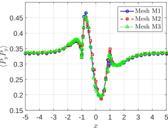
3.26 The flow past a cylinder in a channel. The distribution of PyPy
of the orientation tensor hPPi along the centreline y= 0 and the cylinder’s surface. . . 118 3.27 The flow past a circular cylinder in a channel using Mesh M3: The
contour values of the xx-, xy- and yy-components of the tensor
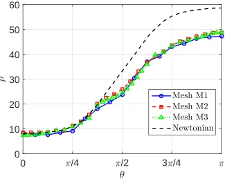
hPPi around the cylinder. . . 119 3.28 The flow past a cylinder in a channel: The distribution of pressure
on the cylinder’s surface. . . 120 3.29 The flow past a cylinder in a channel: The evolution of the drag
force per unit length exerted on the cylinder using three meshes M1, M2 and M3. . . 120
4.1 Flow through two parallel plates: the geometry of the problem. 136 4.2 A grid convergence study for flow with kf = 12: the convergence
measure of the velocity field for grids M1, M2, M3, and M4. . 139 4.3 A grid convergence study for flow withkf = 12: the axial velocity
distribution on the centreline (figure (a)) and the distribution of the extra shear stress at the outlet (figure (b)) for grids M1, M2, M3, and M4. . . 140 4.4 Flow through two parallel plates: a uniform Cartesian grid. . . 141 4.5 Orientation of fibres: a) Circle: the fibres’ direction is isotropic; b)
Ellipse: the major axis is the predominant direction of fibres and c) Straight line: all fibres completely align with the line. . . . 141 4.6 Fibre suspension flow between two parallel plates: the evolution of
fibres’ orientation along the channel with kf = 2 (figure (a)) and
kf = 10 (figure (b)). . . 141
4.7 Fibre suspension flow between two parallel plates: the distribu-tion of components P1111 (figure (a)) and P1122 (figure (b)) of the
fourth-order orientation tensor on several vertical planes (xi =
{0.05,0.15,0.25,0.5,0.75,1,1.25,2.5,5,7.5,10}) with respect to y using kf = 10. . . 142
List of Figures xxi
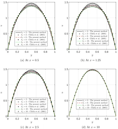
4.9 Fibre suspension flow between two parallel plates: the effect of the fibre parameterkf on the axial velocity profiles at several sections
x∈ {0.5,1.25,2.5,10} of the channel. . . 144 4.10 Fibre suspension flow between two parallel plates: the distribution
of shear stress in the fibre suspension flow with kf = 10 (figure
(a)). Figure (b) has been extracted from Fig. 8(a) on page 154 of Chiba et al. (2001) for comparison. . . 146 4.11 Fibre suspension flow between two parallel plates: the distribution
of the first normal stress difference (figure (a)) in the fibre suspen-sion flow with kf = 10. Figure (b) has been extracted from Fig.
9(a) on page 155 of Chiba et al. (2001) for comparison. . . 146 4.12 Fibre suspension flow between two parallel plates: the convergence
measure for vorticity, stream function and velocity fields of flows with kf = 2 (figure (a)) and kf = 10 (figure (b)). . . 147
4.13 Fibre suspension flow between two parallel plates: the convergence measure for vorticity (figure (a)), stream function (figure (b)) and velocity field (figure (c)) of flows using several fibre configuration fields Nf ∈ {180,270,360,450,540}. . . 148
4.14 Fibre suspension flow through a circular tube: the geometry of the problem. . . 149 4.15 Fibre suspension flow through a circular tube: a non-uniform
Carte-sian grid for the problem. . . 151 4.16 Fibre suspension flow through a circular tube: the centreline
ve-locity profiles of flows withkf ∈ {2,6,10}(solid lines). The
corre-sponding results for the fibre suspension flow between two parallel plates presented in Section 4.7.1 are also reproduced in dashed-line form for comparative purpose. . . 152 4.17 Fibre suspension flow through a circular tube: the undershoot
value of the centreline velocity profiles for the fibre suspension flows with kf ∈ {2,4,6,8,10,12}. The corresponding results of
List of Figures xxii
4.18 Fibre suspension flow through a circular tube: the distribution of shear stress (figure (a)) and the first normal stress difference (figure (b)) for the case of fibre parameter kf = 10. . . 154
4.19 Fibre suspension flow through an axisymmetric contraction: A schematic geometry for the 4:1 and 4.5:1 axisymmetric contraction flows. . . 155 4.20 Fibre suspension flow through an axisymmetric contraction: a
non-uniform Cartesian grid for the 4:1 axisymmetric contraction flow. 156 4.21 The axisymmetric 4:1 contraction flows of fibre suspensions: the
effect of the fibre parameter on the vortex length (L∗
v) with a range
of kf ∈ {0,1, . . . ,11,12} for the flows with Re = 0 and kf ∈
{0,1, . . . ,7,8} for the flows with Re= 1. . . 158 4.22 The axisymmetric 4:1 contraction flows of fibre suspensions: the
effect of the fibre parameter on the streamlines and the vortex of the velocity field for the flows with Re = 0 and a range of kf ∈ {0,4,8,12}. . . 159
4.23 The axisymmetric 4:1 contraction flows of fibre suspensions: the distribution of the fibres’ orientation around the contraction area for the flows with Re= 0 and a range of kf ∈ {0,4,8,12}. . . 160
4.24 The axisymmetric 4:1 contraction flows of fibre suspensions: the effect of Reynolds number on the streamlines and vortices of the velocity field for a range of Re∈ {0,1,2,5}and kf = 6. . . 161
4.25 The axisymmetric 4:1 contraction flows of fibre suspensions: The axial velocity profile on the centreline for a range ofkf ∈ {0,4,8,12}
and Re= 0. . . 162 4.26 The axisymmetric 4:1 contraction flows of fibre suspensions: The
velocity gradient profile on the centreline for a range of kf ∈
{0,4,8,12}and Re= 0. . . 163 4.27 The axisymmetric 4:1 contraction flows of fibre suspensions: The
first normal stress difference on the centreline for a range of kf ∈
List of Figures xxiii
4.28 The axisymmetric 4.5:1 contraction flows of fibre suspensions: the effect of the fibre parameter on the vortex length (L∗
v) for a range
of kf ∈ {0,1, . . . ,7,8} and Re= 0. . . 164
5.1 Orientation of fibres: a) Circle: the isotropic fibres’ direction; b) Ellipse: the major axis is the predominant direction of fibres and c) Straight line: all fibres completely align with the line. This figure is from Chapter 4. . . 176 5.2 Non-dilute fibre suspension flow through a circular tube: the
ge-ometry. . . 177 5.3 Non-dilute fibre suspension flow through a circular tube: the
non-uniform Cartesian grid discretisation. . . 177 5.4 Non-dilute fibre suspension flow through a circular tube: theuz
ve-locity profile along the centreline of flows withφa2
r ∈ {1,5,10,15,20}. 179
5.5 Non-dilute fibre suspension flow through a circular tube: the effect of fibre parameters on the velocity profile along the fibre direction with φa2
r = 1 (figure (a)); φa2r = 10 (figure (b)); and φa2r = 20
(figure (c)). . . 181 5.6 Non-dilute fibre suspension flow through a circular tube: the
ve-locity profiles at the outlet of the channel for flows with φa2
r ∈
{1,5,10,15,20}. . . 182 5.7 Non-dilute fibre suspension flow through a circular tube: the
stream-lines for the cases of Newtonian fluid (figure (a)), fibre suspensions with φa2
r = 5 (figure (b)) and φa2r = 20 (figure (c)) in the domain
z ∈[0,4]. . . 182 5.8 Non-dilute fibre suspension flow through a circular tube: the
con-tour of the extra shear stress (τezr) for the flows with φa2r = 5
(figure (a)) and φa2
r = 20 (figure (b)) in the domain z ∈[0,4]. 183
5.9 Non-dilute fibre suspension flow through a circular tube: the con-tour of the first normal stress difference (τzz
e −τerr) for the flows
with φa2
r = 5 (figure (a)) and φa2r = 20 (figure (b)) in the domain
List of Figures xxiv
5.10 Non-dilute fibre suspension flow through a circular tube: the con-vergence measure for velocity (figure (a)), stream function (figure (b)) and vorticity (figure (c)) of flows withφa2
r ∈ {1,5,10,15,20}. 184
5.11 A schematic geometry for the axisymmetric contraction flow. . 185 5.12 A non-uniform Cartesian grid for the 4:1 axisymmetric contraction
flow. . . 186 5.13 The 4:1 axisymmetric contraction flows of non-dilute fibre
suspen-sions: the effect of fibre parameters on the vortex length (L∗
v) with
ar = 10 and a range ofφ∈ {0.01,0.02,0.05,0.08,0.10,0.12,0.15,0.18,0.20};
and ar = 20 and a range of φ∈ {0.01,0.02,0.05,0.08,0.10}. . . 187
5.14 The 4:1 axisymmetric contraction flows of non-dilute fibre sus-pensions: the effect of φa2
r on the salient corner vortex size for
φa2
r ={5,10,15,20}. . . 188
5.15 The 4:1 axisymmetric contraction flows of non-dilute fibre suspen-sions: the orientation of fibres around the contraction area for φa2
r{5,10,15,20}. . . 190
5.16 The 4:1 axisymmetric contraction flows of non-dilute fibre suspen-sions: the effect of Reynolds number (Re) on the salient corner vortex for φa2
r = 12. . . 191
5.17 A schematic geometry for the 1:4 axisymmetric expansion flow. 192 5.18 A non-uniform Cartesian grid for the 1:4 axisymmetric expansion
flow. . . 193 5.19 The 1:4 axisymmetric expansion flows of non-dilute fibre
suspen-sions: the effect of fibre parameters on the vortex length (L∗
v) for
ar = 10 and a range ofφ∈ {0.01,0.02,0.05,0.08,0.10,0.12,0.15,0.18,0.20};
and ar = 20 and a range of φ∈ {0.01,0.02,0.05,0.08,0.10}. . . 194
5.20 The 1:4 axisymmetric expansion flows of non-dilute fibre suspen-sions: the effect of φr2a on the salient vortex pattern for φa2r ∈
{5,10,15,20}. A lip vortex appears for higher values of φa2
r. . 195
List of Figures xxv
5.22 The 1:4 axisymmetric expansion flows of non-dilute fibre suspen-sions: the effect of the Reynolds number on the salient corner vortex for ar = 10 and φ= 0.12. . . 198
5.23 The 1:2 axisymmetric expansion flows of non-dilute fibre suspen-sions for ar = 10 and φ = 0.15: the evolution of fibre stresses
including shear stress (τzr
f ), normal stresses (τfzz and τfrr) and the
first normal stress difference (τrr
f −τfzz) at position z = 5.75 and
r= 0.5. . . 199
6.1 Start-up planar Couette flow problem: the bottom plate moves with a constant velocity V = 1, the top plate is fixed; no slip boundary conditions apply at the fluid-solid interfaces. The collo-cation point distribution is only schematic. . . 205 6.2 Start-up planar Couette flow using a Hookean dumbbell model
fluid: Discretisation of a 2-D bounded domain (bi-periodic do-main) of the micro configuration space {X, Y} developed at a lo-cation pointyj of the Couette flow problem. The collocation point
distribution is only schematic. . . 208 6.3 Start-up planar Couette flow using a Hookean dumbbell model
fluid: the parameters of the problem are number of dumbbells N = 625, number of collocation points Ny = 21, ∆t = 0.01,
Weissenberg Number W e = 0.5, Reynolds number Re = 0.1 and the ratio ε = 0.9. The evolution of the velocity at locations y∈ {0.2,0.4,0.6,0.8}in comparison with the results of the IRBF-BCF multiscale method by Tran et al. (2011). . . 209 6.4 Start-up planar Couette flow using a Hookean dumbbell model
fluid: the parameters are shown in Fig. 6.1 and the caption of Fig. 6.3. The evolution of shear stress at the locations y ∈
List of Figures xxvi
6.5 Start-up planar Couette flow using a Hookean dumbbell model fluid: the parameters are shown in Fig. 6.1 and the caption of Fig. 6.3. The evolution of shear stress at the locations y ∈
{0.2,0.4,0.6,0.8}in comparison with the results of the IRBF-BCF multiscale method by Tran et al. (2011). . . 210 6.6 a) Start-up planar Couette flow problem using the FENE dumbbell
model; b) Discretisation of a 2-D bounded domain of the micro configuration space X, Y developed at a location point yj: the
collocation point distribution is only schematic.. . . 211 6.7 Start-up planar Couette flow using FENE dumbbell model fluid:
the evolution of velocity at locationsy∈ {0.2,0.4,0.6,0.8}. . . 212 6.8 Start-up planar Couette flow using FENE dumbbell model fluid:
List of Tables
2.1 The creeping planar Couette flow problem using the FENE-based BSC model of 1, 3 and 6 dumbbells. The parameters of the problem are given in Fig. 2.5. An evaluation of the numerical stability of the present method: the statistical errors of the shear stress and the first normal stress of the present method are compared with those of Koppol et al. (2007). S[τxy] and S[τxx] are the statistical
errors of the shear stress and the first normal stress, respectively. 60 2.2 The start-up planar Couette flow problem using FENE-BSC
mod-els with HI and EV effects. The parameters of problem: number of dumbbells in a BSC Ns = 2, number of BSC configurations at
each collocation point Nf = 1024, ∆t = 0.001, number of
itera-tions it = 2.5E + 4. Parallel computation results are shown in the table where CPUs is number of CPUs, tm is elapsed time for
the micro procedure, tM is elapsed time for the macro procedure,
S is single mode, P is parallel mode, Spd is speed-up and Eff is efficiency. . . 75
3.1 Simulation of the start-up Couette flow of polymer melt using the DE, CB, RR, DR models. Parameters of 16 different cases includ-ing six cases of the CB model (CBT1 -CBT6), six cases of the RR
model (RRT1 - RRT6) and three cases of the DR model (DRT1
-DRT3) are derived from the DE model with λ = 50, ηo = 1 and
l3 = 0; G=NnpkBT: the rigidity modulus of models. Parameters
List of Tables xxviii
3.2 The flow past a circular cylinder in a channel. The parameters of the three grids M1, M2 and M3. ∆x1: the grid spacing in
x-direction ∀x ∈ [−15,−5]S[5,15], ∆x2 ∀x ∈ [−5,−2]S[2,5], ∆x3
∀x ∈ [−2,−1]S[1,2]; ∆y: the grid spacing in y-direction; Ncyn:
the number of collocation points on the cylinder’s surface and N: the number of collocation points on the whole domain. . . 112
4.1 A grid convergence study for the fibre suspension flow between two parallel plates. Four different grids are used where ∆xand ∆yare grid spaces inx-direction andy-direction, respectively; andNx and
Ny the number of grid nodes in each direction. . . 138
4.2 Fibre suspension flow between two parallel plates. A study for the stability of the present method based on the fibre parameter kf
and the time step size ∆t for grid M3. The figures shown in the table are the values of the convergence measure of the velocity field (CM(u)) at t = 10. ‘X’ is a divergent measure. . . 139 4.3 Fibre suspension flow through a circular tube. Value and distance
from the inlet boundary of undershoots appearing in the centreline velocity profiles with kf ∈ {2,6,10}. Results for planar flows are
included for comparative purpose. . . 152
5.1 Fibre suspension flow through a circular tube. States of fibre sus-pension fluids: dilute (φa2
r < 1), semi-dilute (1 ≤ φa2r < ar) and
concentrated (φa2
r ≥ ar). ar: the aspect ratio of fibre, φ: the
vol-ume fraction, and (·)∗: the value of (·) associated with a
r = 20. 176
5.2 Fibre suspension flow through a circular tube: A study for the stability of the present method with respect to time step size using the non-uniform grid described in Fig. 5.3. Convergence measures of the velocity field (CM(u)) at t= 10 for different ∆t’s and fibre parameters (φa2
Chapter 1
Introduction
1.1
Motivation, significance and objectives
Simulation of transient non-Newtonian fluid flows, e.g. flows of viscoelastic fluid or fibre suspensions, plays a very important role in several manufacturing indus-tries, for example, processing of polymer liquids (dilute or concentrated solutions and melts) (Barone and Tucker, 1989) and fibre-reinforced composite materials (Folkes, 1982). The simulation in these fields is practically interesting but compu-tationally challenging. Although the macroscopic simulation for the evolution of non-Newtonian flows has achieved significant progresses over the last five decades, the approach is deficient in solving several real flow problems in terms of both geometry and materials, for example, moving boundary and free surface for com-plex geometry and lack of closed-form constitutive equation for comcom-plex fluid. Hence, any computational achievement in solving such problems will advance the simulation method and bring enormous benefits to industry.
1.2. Governing equations 2
fields which satisfy the physical conservation equations while on the micro-scale, it is necessary to use kinetic theory to get a more detailed material description in terms of the probability distribution function of particles (Bird et al., 1987b). This approach is known as the continuum-microscopic multiscale method and does not require closed-form constitutive equations (Ottinger, 1996). More recently, the Computational Engineering and Science Research Centre, University of Southern Queensland, has developed radial basis function networks (RBFNs) based numer-ical methods for the simulation of stochastic multiscale macro-micro models of fluids (Tran-Canh and Tran-Cong, 2002b, 2004; Tran et al., 2011, 2012a). Our research is a further development of this approach with the main objectives as follows.
1. To devise multiscale simulation approaches, incorporating the IRBF ap-proximation scheme, which will be both accurate and efficient, for the sim-ulation of a system of hybrid governing equations of non-Newtonian flows;
2. To apply the new methods for the solution of complex fluid flows using various kinetic models such as the Bead Spring Chain (BSC) models for dilute polymer solutions and reptation models for concentrated polymer solutions and polymer melts; and
3. To develop efficient computational procedures based on the BCF coarse grained method and RBF schemes for the simulation of fibre suspension flows in both dilute and non-dilute regimes.
1.2
Governing equations
1.2. Governing equations 3
1.2.1
Conservation equations
It is known from continuum fluid mechanics that the physical behaviour of a fluid is completely governed by a set of conservation equations of mass, momentum and energy as follows (Bird et al., 1987a).
• Equation of continuity Dρ
Dt +ρ(∇ ·u) =0, (1.1)
• Equation of motion
ρDu
Dt = (∇ ·σ) +ρb, (1.2)
• Equation of energy
ρDe
Dt =−(∇ ·q)−(σ :∇u), (1.3) where u is the velocity vector; t the time; ρ the density of the fluid; σ the total
stress tensor; b and e the body force and the internal energy per unit mass, respectively; andqthe heat flux vector. D/Dtis the substantial or material time derivative associated with a specific fluid element (•) and defined as
D
Dt(•) = ∂(•)/∂t+u· ∇(•). (1.4) The total stress tensor σ for a given fluid can be decomposed as
σ =−pI+τe, (1.5)
where pis the hydrostatic pressure; I the identity tensor; andτe the extra stress
tensor which is defined by means such as constitutive relations.
1.2. Governing equations 4
momentum (1.1)-(1.2) with no body force (b = 0) are rewritten as follows.
∇ ·u =0, (1.6)
ρ
∂u
∂t +u· ∇u
=−∇p+∇ ·τe. (1.7)
1.2.2
Constitutive equations
The constitutive equation derived from experimental observations or theoretical principles describes the relation between the stress tensor and the flow kinematics. Several constitutive equations are summarised as follows.
Newtonian fluids
For a Newtonian fluid, the extra stress tensor τe in Eq. (1.5) is replaced by the
Newtonian stress tensor τs, which is defined by the stress-strain relation of the
fluid as
τs= 2ηsD, (1.8)
where ηs is the fluid constant viscosity; D = 12(∇u + (∇u)T) the fluid
defor-mation rate tensor; and ∇u and (∇u)T the velocity gradient and its transpose,
respectively.
Polymeric fluids (solutions and melts)
For a polymeric fluid, the extra stress tensor τe consists of two components, one
contributed by the polymer and the other by a Newtonian matrix. Therefore, the total stress tensor in Eq. (1.5) is rewritten as follows.
σ =−pI+τs+τp, (1.9)
where τp is the polymer contributed stress caused by the evolution of
1.2. Governing equations 5
equation for a polymeric fluid is given by
ρ
∂u
∂t +u· ∇u
=−∇p+∇ · τs+τp
. (1.10)
Several common constitutive equations, which are listed below, are used to de-termine the polymer-contributed stress τp.
• Upper-convected Maxwell (UCM) model
The linear UCM model was derived by Oldroyd (1950) as follows.
τp+λ
△
τp = 2ηpD, (1.11)
where λ is the relaxation time; ηp the polymer-contributed viscosity; and
△
τp the upper-convected derivative of the polymer stress tensor. In general,
the upper-convected derivative for any second-order tensorA is defined by (Oldroyd, 1950)
△
A= ∂A
∂t +u· ∇A−(∇u)
T
·A−A· ∇u. (1.12)
• Oldroyd-B model
A combination of the Newtonian solvent stress and the polymer stress in the UCM model yields the Oldroyd-B model (Bird et al., 1987a)
τe+λ1
△
τe = 2η0
D+λ2
△ D
, (1.13)
where λ1 is the relaxation time; λ2 =λ1ηηs0 the retardation time; and η0 =
ηs+ηp the total viscosity. It should be noted that the Oldroyd-B model
reduces to the Newtonian fluid forλ2 =λ1 and the UCM model forλ2 = 0.
• Phan-Thien–Tanner (PTT) models
1.2. Governing equations 6
– The linear PTT model (Phan-Thien and Tanner, 1977)
1 + λ1ǫ ηp
tr τp
!
τp+λ1
△
τp+ξλ1 τp ·D+D·τp
= 2ηpD, (1.14)
where ǫ and ξ are the adjustable parameters of the model and deter-mined from experiments; and tr(∗) the trace of (*).
– The exponential PTT model (Phan-Thien, 1978)
exp λ1ǫ ηp
tr τp
!
τp +λ1
△
τp+ξλ1 τp·D+D·τp
= 2ηpD. (1.15)
Other constitutive equations in the literature such as the differential Pom-Pom model for branched polymer melt systems and the integral K-BKZ model for polymer melts can be found in Bird et al. (1987b); Aksel (2002); McLeish and Ball (1986) and Tanner (1988).
Fibre suspensions
For fibre suspensions with a Newtonian solvent, the extra stress tensor τe is
decomposed into two components: the Newtonian solvent stress τs and the
fibre-contributed stress τf. As a result, the total stress formulation (1.5) and the
momentum equation (1.7) are rewritten for fibre suspensions as follows.
σ =−pI+τs+τf, (1.16)
ρ
∂u
∂t +u· ∇u
=−∇p+∇ ·τs+∇ ·τf. (1.17)
It is worth noting that there is no closed-form constitutive equation for fibre suspensions without using closure approximations (Fan, 2006; Lu et al., 2006; Chinesta and Ausias, 2015). Therefore, most fibre stress formulations were de-rived in terms of the orientation of fibre configurations, which is basically char-acterised by a unit vector P along the fibre’s axis.
1.2. Governing equations 7
suspensions are briefly described as follows.
• Transversely isotropic fluid (TIF) model for dilute suspensions The TIF model of an anisotropic fluid was first proposed by Ericksen (1960) and then derived by Hinch and Leal (1975) for dilute suspensions from the theory of microstructures. The particle/fibre-contributed stress by the TIF model is determined as follows (Hinch and Leal, 1976).
τf = 2ηsφ
n
AhPPPPi:D+B D· hPPi+hPPi ·D +CD+DrF hPPi ,
(1.18)
where P is the unit vector directed along a suspended particle; PPPP andPPthe fourth-order and second-order orientation tensors ofP, respec-tively; (∗) the statistical average of (∗); φ the fibre volume fraction of the suspension; Dr the rotational diffusivity coefficient; ar = dlff the aspect
ratio of the fibre; and A, B, C and F functions of ar. For a suspension
of high aspect ratio fibres, these coefficients are given by (Phan-Thien and Graham, 1991)
A= a
2
r
2 (ln2ar−1.5)
, B = 6ln2ar−11 a2
r
,
C = 2, F = 3a
2
r
ln2ar−0.5
.
(1.19)
• Lipscomb model for dilute suspensions
Lipscomb et al. (1988) has transformed the TIF constitutive equation into a coordinate system which instantaneously coincides with the major axes of the ellipsoid particle. The corresponding fibre-contributed stress for non-Brownian suspensions of high aspect ratio fibres is determined as (Lipscomb et al., 1988)
τf =
φµ ηs h
PPPPi:D, (1.20)
whereµis the material constant defined asµ=ηsa2r/lnarwith a sufficiently
1.2. Governing equations 8
• Dinh-Armstrong model for semi-concentrated suspensions
The model was developed to approximate the fibre stress for semi-concentrated stiff fibre suspensions with a Newtonian solvent whose volume fraction is in the range 1/a2
r,1/ar
(Dinh and Armstrong, 1984). The fibre stress formulation of this model is given by
τf = 2ηsD
" 1 48
nfl3f
ln(2hf/df)
: Z
PPPP (1 +γ0 :PP)1.5
dP #
, (1.21)
where nf is the fibres density; γ0 the infinite strain tensor; and hf the
pa-rameter representing the average distance from a fibre to its nearest neigh-bour. Other parameters was defined as above. More details of the model can be found in Dinh and Armstrong (1984).
• Phan-Thien–Graham model for concentrated suspensions
A constitutive equation for suspensions with rod-like particles whose aspect ratio is in the range [5,30] has been proposed by Phan-Thien and Graham (1991). The equation neglects the Brownian motion of fibres and only considers the dominant term related to the fourth-order orientation tensor PPPPin the TIF model. The fibre-contributed stress tensor is determined as (Phan-Thien and Graham, 1991)
τf = 2ηsf(φ, ar)D :hPPPPi. (1.22)
The function f(φ, ar) in Eq. (1.22) is given by
f(φ, ar) =
a2
rφ(2−φ/φm)
4(ln2ar−1.5)(1−φ/φm)2
, (1.23)
where φm is the maximum volume fraction of the suspension and
approxi-mated based on the experimental results of Kitano et al. (1981) as
φm = 0.53−0.013ar, 5< ar <30. (1.24)
1.3. Simulation of polymeric fluids 9
modified Phan-Thien–Graham model (Fan et al., 1999)
τf =ηsf(φ) AD:hPPPPi+DrF hPPi
, (1.25)
where A and F are the parameters as defined in Eq. (1.19); and f(φ) is now given by
f(φ) = φ(2−φ/φm) 2(1−φ/φm)2
. (1.26)
In this research project, the Phan-Thien–Graham model is used to approximate fibre stress in the simulation of concentrated fibre suspension flows.
1.3
Simulation of polymeric fluids
Generally, there are two common approaches for simulations of flows of polymeric fluid: the purely macroscopic approach and the macro-micro multiscale approach. The two simulation approaches are similar in integrating the effect of polymer phase in the motion equation of the flow but distinctively different in the manner of calculating the polymer stress. Indeed, the polymer-contributed stress is ob-tained by solving the constitutive equation in the macroscopic approach whereas it is computed from the information of micro-structures, which represent the real polymer molecules, in the macro-micro approach.
1.3.1
Macroscopic approach
1.3. Simulation of polymeric fluids 10
Phillips, 2002; Engquist et al., 2009).
1.3.2
Macro-micro multiscale approach
In the macro-micro multiscale approach or the coarse-grained (CG) simulation, there are two separate procedures which need to be carried out at each time step: the macro and micro procedures. In the macro procedure, the kinetic behaviour of the flow is governed by the conservation equations for mass and momentum. Meanwhile, in the micro procedure, the dynamic behaviour of polymeric liquids is described based on the micro-configuration/structure of polymers using kinetic CG models. The governing equations in the two procedures are then linked together by the Kramers expression, which is used to calculate the polymer stress from the configurations of polymer models in the micro procedure.
meth-1.3. Simulation of polymeric fluids 11
ods are studied in this thesis, the SDE-based method is the main focus of our research project. The SDE simulation method can be classified into two main groups: the Lagrangian BDS and the Eulerian BDS.
The Lagrangian BDS was developed by Ottinger and Laso (Laso and Ottinger, 1993) (named as the Calculation Of Non-Newtonian Flows: Finite Elements & Stochastic Simulation Techniques (CONNFFESSIT)). The main idea of the CON-NFFESSIT is that the polymer-contributed stress is averagely calculated from the configurations of a large ensemble of microstructures, which describe poly-mer chains existing in the polypoly-mer solution (Bird et al., 1987b; Ottinger, 1996). Thus, there is no need for a closed form constitutive equation. However, there are several challenges for the method, including: (i) the stochastic noise in the solution of the fibre stress and (ii) particle tracking of a huge number of particles at each time step.
Hulsen et al. (1997) have later proposed the Eulerian BDS scheme, also known as the Brownian configuration field (BCF) technique. The BCF’s main idea is that the collection of discrete particles in the CONNFFESSIT is replaced by an ensemble of continuous configuration fields. These configuration fields are convected and deformed by the drift components (the velocity gradient of flow and elastic forces) and the Brownian diffusion motion during the simulation. Owing to the Eulerian nature, the variance reduction techniques and parallel processing simulations can be set up easily in the BCF-based algorithm (Ottinger et al., 1997).
1.3. Simulation of polymeric fluids 12
Figure 1.1: An illustration of 5-bead chain of multi BRS models.
Bead-rod-spring (BRS) models for dilute polymer solutions
For these kinetic models, beads are considered as mass points, rods are massless and have a fixed length, and the pendant hydrogen atoms are reduced for sim-plicity. Generally, BRS models are divided into two basic subclasses. The first group consists of the freely rotating chain model and the freely jointed multi-bead-rod chain model (or the Kramers chain) (Fig. 1.1 - left figure). In the second group, beads are connected by springs, forming the freely jointed bead-spring chain model (Fig. 1.1 - right figure). The model offers some advantages over the corresponding bead-rod model, e.g. the internal constraints are not considered in the bead-spring model. However, it also suffers from some disadvantages. For example, the chain length is not bounded, especially if the extension of spring is governed by the Hookean law, the polymer chain can be stretched unlimitedly in shear flow. The simplest form of the BRS models is the dumbbell model with 2 beads. More details of BRS models can be found in Bird et al. (1987b); Cruz et al. (2012).
1.3. Simulation of polymeric fluids 13
existence of the second normal stress difference or the shear dependence of vis-cometric functions are forecasted accurately (Zimm, 1956). Thus, the obtained results by the simulation now are able to be compared with those achieved by experiments. Recently, a number of significant advancements of the BRS models have been developed to fully examine the effects of the intramolecular forces on the motion of molecular chains (Ottinger, 1987b, 1989b; Zylka, 1991; Prakash, 2002).
Reptation models for concentrated polymer solutions and polymer melts
1.4. Simulation of fibre suspensions 14
1.4
Simulation of fibre suspensions
In this thesis, fibre suspension flows are simulated with the assumptions as follows. (i) fibres are rigid, rod-like particles, and (ii) the fluid is homogeneous because of a constant volume fraction on the whole investigated domain. Two character-istic parameters of the fibres are the aspect ratio ar and the volume fraction φ,
which is defined as the total volume of fibres as a fraction of the total volume of suspension. The constitutive equations for fibre suspensions (Section 1.2.2) are formed in terms of statistical averages of the orientation tensors (PPPPand PP) and it is not easy to derive deterministic closed-form constitutive equations in terms of material properties and standard kinematic quantities. Therefore, in order to close the system, it is necessary to establish an evolution equation for fibres’ orientation P’s and a formulation to determine the orientation tensors. A discussion on these issues is as follows.
1.4.1
Evolution equation
Jeffery (1922) has introduced the motion equation of a single ellipsoidal particle as
dP
dt =Ω·P+λ(D−D:PPI)·P, (1.27) where Ω= 12 (∇u)T − ∇uis the vorticity tensor; and λis a parameter depen-dent on the ellipsoidal aspect ratio and given by λ= (a2
r−1)/(a2r+ 1).
This equation has been later used extensively by rheologists to simulate fibre suspensions in dilute regime (Goettler et al., 1979, 1981; Givler, 1981; Givler et al., 1983; Lipscomb et al., 1988; Chiba et al., 1990).
1.4. Simulation of fibre suspensions 15
equation. By experimental observations, Folgar and Tucker (1984) proposed an evolution equation with the effect of fibre-fibre interactions for the description of non-dilute suspensions as follows.
dP
dt =Ω·P+λ(D−D :PPI)·P− Dr
ψ ∇Pψ, (1.28)
whereψ is the probability distribution function ofP (ψ =ψ(P, t) for the homo-geneous suspensions); and∇P the gradient operator associated withP. Dr is the
rotational diffusivity coefficient and approximated by (Folgar and Tucker, 1984).
Dr =Ciγ,˙ (1.29)
where ˙γ =p2 (D :D) is the general strain rate; andCithe interaction coefficient,
namely the Folgar-Tucker constant.
The diffusion equation or the FPE derived from Eq. (1.28) for fibre suspensions is given by (Folgar and Tucker, 1984)
∂ψ ∂t =
∂ ∂P
n
ψΩ·P+λ(D−D:PPI)·Po+Ciγ˙
∂2ψ
∂P2. (1.30)
The stochastic version of the FPE (1.30) is written as follows (Fan et al., 1999)
dP
dt =L·P−L :PPP+ (I−PP)·F
(b)(t), (1.31)
where L is the effective velocity gradient tensor and given by L = (∇u)T −ζD with ζ = 2/(a2
r + 1) and ζ = 1−λ. The Brwonian force F(b)(t) possesses the
properties DF(b)(t)E= 0 and DF(b)(t+s)F(b)(t)E = 2D
rδ(s)I where δ(s) is the
Dirac delta function. The Brownian force is a function of white noise and given by (Ottinger, 1996).
F(b)(t) =p2Ciγ˙
dW
dt , (1.32)
where Wis a Wiener process. Substituting Eq. (1.32) into Eq. (1.31) yields the evolution equation for non-dilute fibre suspensions as follows.
dP
dt =L·P−L :PPP+ p
2Ciγ˙ (I−PP)·
dW
1.4. Simulation of fibre suspensions 16
where the interaction coefficient Ci 6= 0. Eq. (1.33) becomes the Jeffery equation
(1.27) for dilute fibre suspensions with Ci= 0 (Phan-Thien and Graham, 1991)
1.4.2
Simulation methods
The general procedure for the simulation of fibre suspensions consists of three steps as follows: Firstly, solve the conservation equations with a known fibre stress to update the velocity and pressure fields; Secondly, solve the evolution equation with the updated pressure and velocity fields to determine the fibres’ configuration of the current time step; Lastly, calculate the fibre stress field from the updated configuration of fibres. Follow this procedure, several simulation methods have been devised to predict dynamic behaviours of fibre suspension flows. The methods differ mainly in the way to proceed the last two steps in the procedure. Generally, these methods can be classified into several main ap-proaches as follows.
Closure approximation
In this approach, instead of solving the evolution equation for the unit orientation vectorP, ones solve the evolution equation for either the second-order or fourth-order tensors of P. The evolution equation for the second-order tensor of P is given by
dhPPi
dt =L· hPPi+hPPi ·L
T
−2L :hPPPPi +2Ciγ˙ I−αdhPPi
,
(1.34)
where αd is the number of dimension of fibre, i.e. αd= 2 for 2-D orientation and
αd = 3 for 3-D orientation. Since Eq. (1.34) also includes the unknown
fourth-order orientation tensorhPPPPi, it is not a closed form. Therefore, many closure approximations have been proposed to approximate the fourth-order orientation tensor from the second-order one.
Let Pijkl = hPPPPi and Pij =hPPi be the fourth-order and the second-order
1.4. Simulation of fibre suspensions 17
developed as follows.
• The linear closure approximation (Hand, 1962),
ˆ Pijkl ≃
1 4 +αd
Pijδkl+Pikδjl+Pilδjk+Pklδij+Pjlδik+Pjkδil
−(4 +α 1
d)(2 +αd)
δijδkl+δikδjl+δilδjk
;
(1.35)
• The quadratic closure approximation (Lipscomb et al., 1988),
˜
Pijkl≃PijPkl (1.36)
• The hybrid closure approximation (Advani and Tucker III, 1987, 1990), which is a combination of the quadratic and linear approximations, is given by
¯
Pijkl ≃(1−f) ˆPijkl+fP˜ijkl, (1.37)
wheref is the scalar measure of orientation and given asf = 1−NdethPPi (Advani and Tucker III, 1990) withN = 4 for 2-D andN = 27 for 3-D fibre’s orientation .
Other advanced closure approximations can be found in several publications by Verleye et al. (1993); Dupret et al. (1997); Cintra Jr and Tucker III (1995); Chung and Kwon (2001, 2002) and Jack et al. (2010).
Statistical scheme
For this approach, the Jeffery equation is integrated along streamlines and the fourth-order orientation tensor at a particular point on the streamlines is directly calculated from the orientation of Nf fibres surrounding that point as follows.
hPPPPi= 1 Nf
Nf
X
i=1
1.4. Simulation of fibre suspensions 18
Eq. (1.38) depicts that there is no need of any closure approximation. The approach were used to successfully simulate several dilute fibre suspension flows such as flow past 1:4 backward-facing step channels and flow between two parallel plates (Chiba and Nakamura, 1998; Chiba et al., 2001)
FPE-based simulation
In this approach, the FPE (1.30) is solved for the probability distribution func-tion ψ(P, t) and the orientation tensors are then calculated using the following formulae (Advani and Tucker III, 1987)
hPPi= Z
P
PPψdP, (1.39)
hPPPPi= Z
P
PPPPψdP. (1.40)
The application of this scheme for complex flows is very challenging because of the complexity in solving PDEs in multidimensional spaces (Ammar et al., 2006, 2007).
BCF-based simulation
This approach is based on the principle of the BCF approach, which was pro-posed by Hulsen et al. (1997) for the multiscale simulation of viscoelastic fluids. Following the approach, a set of Nf fibre configuration fields is used to replace
all individual fibres on the whole domain. Each configuration field is evolved by Eq. (1.33), which is now rewritten under the Eulerian view as follows.
∂P(x, t)
∂t +u· ∇P=L·P−L :PPP+ p
2Ciγ˙ (I−PP)·
dW
dt , (1.41)
1.5. Numerical methods for deterministic PDEs 19
(Lu et al., 2006).
1.5
Numerical methods for deterministic PDEs
From the classical mechanics, most physical phenomena can be described by a set of deterministic partial differential equations (PDEs). The conventional methods such as finite difference method (FDM), finite element method (FEM), boundary element method (BEM) and finite volume method (FVM) had been thoroughly developed and had demonstrated their superior ability in finding the numerical solution of PDEs for various problems in sciences and engineering. Recently, RBFN-based methods have emerged as a powerful tool and have been successfully applied in several research areas.
1.5.1
Finite difference method
1.5. Numerical methods for deterministic PDEs 20
1.5.2
Finite element method
The method was first introduced by Turner et al. (1956) for the solution of struc-tural problems and then applied to solve the Navier-Stokes equations for fluid flow problems in the late 1970s by several authors, including Temam (1977); Chung (1978); Girault and Raviart (1979). In this method, the investigated domain is divided into unstructured finite elements, which are interconnected at points called nodes. The approximate solution of an unknown variable at each node is defined as a linear superposition of known basis functions or shape functions, usu-ally polynomials, and the numerical values of the unknown at all nodes (Hirsch, 2007). In general, an FEM-based discretisation process can be done through two steps: (i) Transform the original differential equations into integral equa-tions, or their weak formulation, using the variational principle or the methods of weighted residual; (ii) Discretise the weak form equations based on the chosen shape functions to obtain a set of algebraic equations for unknowns. The FEMs have been used extensively for the simulation of viscoelastic fluids in both the macroscopic approach (Crochet et al., 1984; Baaijens, 1998; Sandri, 2004; Ganvir et al., 2007; Mu et al., 2010) and the multiscale macro-micro methods (Laso and Ottinger, 1993; Hulsen et al., 1997; Van Heel et al., 1999; Jourdain et al., 2002; Le Bris and Lelievre, 2012; Lipscomb et al., 1988). An advantage of FEM in solv-ing viscous and viscoelastic flows is its capacity in handlsolv-ing complex geometries. However, generating a mesh of elements may be very time-consuming especially for moving boundary or three-dimensional problems. In addition, the method becomes unstable for highly nonlinear problems due to intrinsic errors produced from Galerkin-based approximations (Osswald and Gramann, 2001).
1.5.3
Boundary element method
1.5. Numerical methods for deterministic PDEs 21
advantage of BEM over the element-type methods for problems with complex geometries and in 3D space (Brebbia et al., 1984; Hunter and Pullan, 2001). In this method, an integral equation related to only boundary values needs to be for-mulated from the original PDE using several mechanisms such as the reciprocal theorems combined with the Green function and the method of weighted residual. The approximate solution at the boundary nodes is then obtained from solving the integral equation. The numerical values of the interior nodes can be approxi-mated from the boundary data if required. The BEM has been rapidly developed and broadly applied to various complex engineering problems (Brebbia et al., 1984). In computational rheology, the method has been used successfully to solve several complex flow problems such as the squeeze-film flow (Phan-Thien et al., 1987a), the flagellar hydrodynamics problems (Phan-Thien et al., 1987b), the 3-D extrusion processes (Tran-Cong and Phan-Thien, 1988), the Stokes problems of multiparticle systems (Tran-Cong and Phan-Thien, 1989; Tran-Cong et al., 1990), and the suspension problems (Phan-Thien et al., 1991; Fan et al., 1998). However, while BEM works successfully for linear and mildly nonlinear problems, it is less effective in solving highly non-linear viscoelastic problems (Tanner and Xue, 2002).
1.5.4
Finite volume method
1.5. Numerical methods for deterministic PDEs 22
balance laws are strictly obeyed on each CV, therefore, the governing conserva-tion equaconserva-tions are automatically satisfied on the whole domain in the FVM-based discretisation. The FVM has also been applied extensively to several problems in computational rheology (Mompean and Deville, 1997; Xue et al., 1998; Wachs and Clermont, 2000; Sahin and Wilson, 2008; Fu et al., 2009). However, like the other element based methods (e.g. FDM, FEM, and BEM), FVM is also consid-ered as a low-order interpolation scheme, therefore a huge number of elements are necessary to obtain an accurate solution. This leads to difficulties in solving large-scale problems.
1.5.5
Spectral method
Like in FEM, the discretisation process in spectral method (SM) is also based on the method of weighted residuals, whose two key elements are the trial functions (or basis functions or shape functions in FEM) and the test functions (or weight functions) (Canuto et al., 1988). The trigonometric, Chebyshev and Legendre polynomials are usually used as the trial functions in SM. Unlike FEM where the trial functions are locally defined on each element, these functions in SM are valid on the whole computational domain. As a result, SM outperforms FEM and FDM in terms of solution accuracy and high-order convergence rate but is very limited in handling problems with complex geometry (Gheorghiu, 2007; Canuto et al., 1988). Therefore, there are just a few applications of SM in solving complex fluid flow problems in the literature such as Beris et al. (1992); Avgousti et al. (1993); Sureshkumar and Beris (1995); Bell et al. (1997).
1.5. Numerical methods for deterministic PDEs 23
2002; Lozinski and Chauviere, 2003).
1.5.6
Radial basis function (RBF) methods
Basically, a RBF network can be considered as a universal approximator. In RBF-based methods, the considered domain is discretised by a set of data points which are distributed regularly or randomly and the unknown function and its deriva-tives are approximated by a linear combination of RBFs. The RBF-based meth-ods offer some advantages over some traditional methmeth-ods. Firstly, the method can be referred to as a truly meshless method in the context of the point col-location formulation (Kansa, 1990). Consequently, the time-consuming meshing process in the element-based methods is reduced significantly. Secondly, owing to the use of RBF-based approximations instead of polynomial functions in other methods, the RBFN-based methods can achieve higher order approximation and fast convergence rate for the solution of PDEs (Fasshauer, 2007).
The RBF-based methods for the solution of PDEs can be classified into two main branches: differentiated RBF (DRBF) (Kansa, 1990) and integrated RBF (i.e. IRBF) (Mai-Duy and Tran-Cong, 2001). In the former method, the original unknown function is first approximated by RBFs and then its first and second derivatives are calculated by differentiation. On the other hand, the IRBF meth-ods begin RBF-based approximation at the highest order derivative of the original function. The lower order derivatives and the unknown function are obtained by integration. Several strong points of the IRBF methods over the DRBF counter-parts can be listed as follows. (i) a superior accuracy for the approximation of a function and its derivatives, even with a relatively coarse discretisation (Mai-Duy and Tran-Cong, 2003); and (ii) high convergence rate, good accuracy and easy implementation in solving high-order ordinary differential equations and PDEs (Mai-Duy, 2005; Mai-Duy and Tran-Cong, 2005). Multiquadric (MQ) or thin-plate spline (TPS) functions are usually chosen for their superior performance over other functions (Franke, 1982; Hardy, 1971).
1.5. Nume