Compact approximation stencils based on integrated flat radial basis functions

Compact approximation stencils based on integrated flat

radial basis functions

N. Mai-Duy

, T.T.V. Le, C.M.T. Tien, D. Ngo-Cong and T. Tran-Cong

Computational Engineering and Science Research Centre,

School of Mechanical and Electrical Engineering,

University of Southern Queensland, Toowoomba, QLD 4350, Australia

Submitted to

Engineering Analysis with Boundary Elements

, Feb/2016;

revised (1) Jul/2016; revised (2) Sep/2016; revised (3) Oct/2016

Abstract This paper presents improved ways of constructing compact integrated radial basis function (CIRBF) stencils, based on extended precision, definite integrals, higher-order IRBFs and minimum number of derivative equations, to enhance their performance over large values of the RBF width. The proposed approaches are numerically verified through second-order linear differential equations in one and two variables. Significant improvements in the matrix condition number, solution accuracy and convergence rate with grid refinement over the usual approaches are achieved.

Keywords: compact approximation, local approximation, integrated radial basis function, flat radial basis function

1

Introduction

Radial basis functions (RBFs) have become one of the main fields of research in numerical analysis. It is theoretically proved that RBF networks having one hidden layer are capable of universal approximation [22]. They can represent an arbitrary continuous function within an arbitrarily small error bound. The application of RBFs for the numerical solution of

∗_{Corresponding author E-mail: [email protected], Telephone 46312748, Fax}

ordinary/partial differential equations (ODEs/PDEs) has received a great deal of attention. In RBF methods, the field variables/their derivatives are represented by linear combinations of RBFs, while the differential equations can be discretised by means of point collocation [6,7,23,26,9,8,21], subregion collocation [20,16], weak form [30,15] or inverse form [19].

Several types of RBFs contain a free parameter. This class can exhibit an exponential rate of convergence with the number of RBFs and the RBF’s width [11]. One of the most widely used RBFs is the multiquadric (MQ) function defined as

Gi(x) =

q

(x−ci)T(x−ci) +a2i (1)

where ci and ai are the centre and width of the ith MQ, or

Gi(x) =

p

ǫi(x−ci)T(x−ci) + 1 (2)

where ǫi is the shape parameter. The MQ function becomes increasingly flat when ai → ∞

or ǫi →0.

RBF approximations for the field variable and its derivatives can be constructed through the differentiation (DRBF) [6] or integration (IRBF) [13,24,10,7,25] process. The latter was developed with the aim of avoiding the reduction in convergence rate caused by differen-tiation. It was also found that integration constants provide effective mechanisms for the implementation of multiple boundary conditions [12] and compact approximations [27], and the enhancement of continuity order of the approximate solution across subdomain inter-faces [14]. Numerical experiments indicated that IRBFs converge faster, but produce the interpolation matrix with larger condition number than those by DRBFs.

When only a few RBFs are activated for the approximation at a point (local approximation), there is a significant improvement in the matrix condition number but the solution accuracy is significantly reduced. The latter can be overcome by using compact approximations, where the approximation involves nodal values of not only the field variable but also its derivatives [28,29,31,17,27]. With compact RBF approximations, high levels of the solution accuracy and sparseness of the system matrix can be achieved together. They are capable of providing a very efficient solution to a differential problem. In contrast to global RBF methods, larger values ofaican be employed here. It was shown in [3,2] that the RBF approximation is more

accurate when ai is increased (orǫi is reduced) and the most accurate approximation occurs

before ai approaches infinity (or ǫi → 0). Furthermore, in the limit of ǫi → 0, the RBF

approximation for a set of centres in one dimension reduces to the Largrange interpolating polynomial on that set of nodes [1]. Numerical experiments indicated that the interpolation matrices for local RBF and compact RBF stencils at large values of the RBF width are ill-conditioned and special treatments are needed. Effective treatments for compact RBF Hermite interpolation schemes (differentiated) were reported in, e.g. [31], where the Contour-Pade algorithm is employed. This work presents several simple but effective approaches to extend the working range of ai for compact integrated RBF approximations.

The paper is organised as follows. A brief overview of CIRBF stencils is given in Section 2. In section 3, some numerical investigations are conducted to identify numerical issues due to the use of large values of ai. In section 4, improved constructions for CIRBF stencils to

extend the working range of ai are presented and then numerically verified in analytic tests.

Section 5 gives some concluding remarks.

2

Compact local integrated RBF stencils

Consider a 3-point stencil [x1, x2, x3]. On the stencil, the second derivative of the dependent

variable u is decomposed into

d2_u(x)

dx2 = 3

X

i=1

where {Gi(x)}3i=1 is the set of RBFs and {wi}3i=1 the set of weights to be found. In one

dimension, the multiquadric (MQ) function takes the form Gi(x) =

p

(x−ci)2 +a2i. We

choose the width according to ai = βdi, where β is a scalar and di is the smallest distance

between ci and its neighbours.

Its first derivative and function are then obtained through integration

du(x)

dx =

3

X

i=1

wiHi(x) +C1 (4)

u(x) =

3

X

i=1

wiHi(x) +C1x+C2 (5)

where Hi(x) =

R

Gi(x)dx andHi(x) =

R

Hi(x)dxare integrated basis functions and C1 and

C2 the constants of integration.

For compact approximations, nodal values of the derivative (or the differential equation) at the side nodes of the stencil are also incorporated in the process of converting the RBF space into the physical space. Assuming that the differential equation takes the formd2_u(x)/dx2 ₌

f(x) (f(x) is a prescribed function), the mapping can be constructed as

            u1 u2 u3

d2_u 1

dx2

d2_u 3 dx2             =            

H1(x1), H2(x1), H3(x1), x1, 1

H1(x2), H2(x2), H3(x2), x2, 1

H1(x3), H2(x3), H3(x3), x3, 1

G1(x1), G2(x1), G3(x1), 0, 0

G1(x3), G2(x3), G3(x3), 0, 0

           

| {z }

C             w1 w2 w3 C1 C2             (6)

where C is a 5×5 matrix that will hereafter be called the conversion matrix. Solving (6)

leads to _

           w1 w2 w3 C1 C2            

=C−1

            u1 u2 u3

d2u1

dx2

d2u3

The second derivative of function u at the middle node is thus computed as

d2_u 2

dx2 = [G1(x2), G2(x2), G3(x2),0,0]C

−1

u1, u2, u3,

d2_u 1

dx2 ,

d2_u 3

dx2

T

(8)

or

d2_u 2

dx2 =η1u1+η2u2+η3u3+η4

d2_u 1

dx2 +η5

d2_u 3

dx2 (9)

where d2_u

1/dx2 = f(x1), d2u3/dx2 = f(x3) and {ηi}5_i=1 are known values. In the case

of Dirichlet boundary conditions and the domain represented by a set of N nodes, the collocation of the differential equation at the interior nodes results in the following system

A−→u =−→b (10)

where A is the system matrix of dimensions (N −2)×(N −2),−→u the vector consisting of values ofuat interior nodes and−→b the vector formed by the RHS of the differential equation and the boundary conditions. Like the central finite-difference method, the structure of A

is tri-diagonal and the system can be efficiently solved for the nodal variable values.

3

Numerical investigation

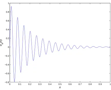
We apply the CIRBF solution procedure to the following second-order ODE

d2_u

dx2 =−exp(−5x) (9975 sin(100x) + 1000 cos(100x)), 0≤x≤1 (11)

subject to Dirichlet boundary conditions. The exact solution can be verified to be

ue(x) = sin(100x) exp(−5x) (12)

and is displayed in Figure 1.

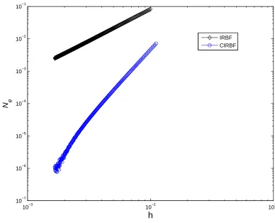
O(h1.95_{) for IRBF, indicating that the inclusion of nodal second derivative values significantly}

enhances the performance of local IRBF stencils.

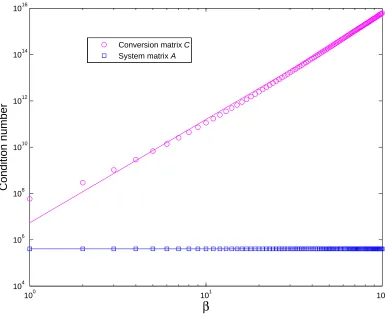
Figure 3 shows variations in the condition number of the conversion and system matrices against the MQ width represented by β for a fixed grid size (Nx = 1001). For the system

matrix A, the condition number is rather low (O(105_{)) and it has similar values over a wide}

range of β. In contrast, the condition number of the conversion matrix C grows fast at a rate of 4.5 and the matrix becomes ill-conditioned at large values of β. Therefore, in using CIRBF stencils, attention should be paid to the handling of matrix C resulting from flat MQ functions.

4

Improved constructions for CIRBF stencils

Below are several treatments proposed to stably compute C at large values ofβ.

4.1

Approach 1: Extended precision

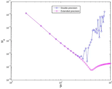
and numerical results indicate that the same level of accuracy is obtained as in the case of using extended precision for the entire computation.

4.2

Approach 2: Definite integral

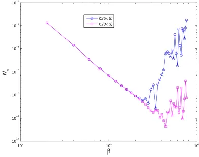
We propose to compute the integrals in their definite form rather than indefinite in con-structing the conversion matrix C. The advantage of this approach is that the size of C is reduced from 5×5 to 3×3, and the numerical stability is thus expected to be improved.

The integrals in (4)-(5) can be rewritten as

du(x)

dx − du1

dx =

3

X

i=1

Z x

x1

wiGi(x)dx

=

3

X

i=1

wi[Hi(x)−Hi(x1)] (13)

u(x)−u1−(x−x1)

du1

dx =

3

X

i=1

Z x

x1

wi[Hi(x)−Hi(x1)]dx

=

3

X

i=1

wi

Hi(x)−Hi(x1)−(x−x1)Hi(x1) (14)

LettingHd

i(x) =Hi(x)−Hi(x1),H

d

i =Hi(x)−Hi(x1)−(x−x1)Hi(x1) andu′(x) =du(x)/dx,

expressions (13) and (14) reduce to

u′(x)−u′₁ =

3

X

i=1

wiHid(x) (15)

u(x)−u1−(x−x1)u′1 = 3

X

i=1

wiH d

i(x) (16)

Our objective now is to express the weights w1, w2 and w3 in terms of u1, u2, u3, u′′1 and u

′′

3.

and x=x3, and the second-derivative expression (3) at x=x1      

u2−u1−(x2−x1)u′1

u3−u1−(x3−x1)u′1

u′′ 1      =      

Hd₁(x1), H

d

2(x1), H

d

3(x1)

Hd₁(x2), H

d

2(x2), H

d

3(x2)

G1(x1), G2(x1), G3(x1)

     

| {z }

C       w1 w2 w3       (17)

Solving this system for the weights yields

      w1 w2 w3     

=C

−₁      

u2−u1−(x2 −x1)u′1

u3−u1−(x3 −x1)u′1

u′′ 1       (18)

A next step is to incorporate u′′

3 into the vector on the RHS of (18). We first collocate the

second-derivative expression (3) at x=x3

u′′

3 = [G1(x3), G2(x3), G3(x3)]C−1

     

u2−u1−(x2−x1)u′1

u3−u1−(x3−x1)u′1

u′′ 1       (19)

and then solving this equation foru′

1. Making substitution into the RHS of (18), the mapping

of the RBF space into the physical space takes the form

      w1 w2 w3     

=C

−1_T

            u1 u2 u3

d2_u 1

dx2

d2_u3

dx2             (20)

where C is of dimension 3×3 and T is of 3×5, which is constructed using results from solving equation (19).

Figure 6 indicates that the present approach makes the solution accuracy significantly less fluctuating over large values of β.

4.3

Approach 3: Higher-order IRBF approximations

The MQ function Gi(x) is now integrated 4 times (IRBF4) instead of twice (IRBF2). Let

Hi(x) =

R

Hi(x)dx, Hbi(x) =

R

Hi(x)dx and Hei(x) =R bHi(x)dx. We employ the integrated

basis function Hi(x) instead of Gi(x) to approximate the second-order derivative

d2_u

dx2 = 3

X

i=1

wiHi(x) (21)

du dx =

3

X

i=1

wiHbi(x) +C1 (22)

u=

3

X

i=1

wiHei(x) +C1x+C2 (23)

where Hbi(x) =

R

Hi(x)dx and Hei(x) =R bHi(x)dx.

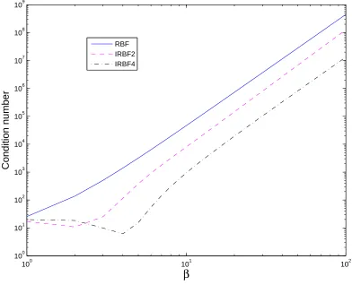
It was reported in [24] that the matrix condition number of IRBF4 is higher than that of IRBF2. However, with only three RBFs involved, the trend is reversed. As RBFs are integrated, the corresponding interpolation matrix has a lower condition number, particularly over a large range of β (Figure 7). When second-derivative values are added, as shown in Figure 8, the observation is similar. CIRBF4 is more stable than CIRBF2. This interesting property of higher-order IRBFs with 3 centres will be utilised here to construct compact IRBF stencils.

The conversion system in this approach is formed as

            u1 u2 u3

d2_u 1

dx2

d2_u 3 dx2             =             e

H1(x1), He2(x1), He3(x1), x1, 1

e

H1(x2), He2(x2), He3(x2), x2, 1

e

H1(x3), He2(x3), He3(x3), x3, 1

H1(x1), H2(x1), H3(x1), 0, 0

H1(x3), H2(x3), H3(x3), 0, 0

           

| {z }

It can be seen from Figure 9 that, for a given β, a much more stable solution is obtained with the present approach as the grid size is reduced. At a very small grid size, the present approach is much more accurate and more stable over a large value range ofβ than the usual approach (Figure 10).

These improved 3-point CIRBF stencils can be extended to construct 5-point stencils for solving problems in two dimensions. The implementation process is exactly the same as that presented in [18]. For elliptic PDEs, the algebraic system, where each row has 5 non-zero entries, can be solved iteratively using a Picard scheme. For parabolic PDEs, systems of tridiagonal equations can be formed and solved efficiently with Thomas algorithm. It requires that the problem domain is represented by a Cartesian grid (not by a set of scattered points). Thus, for non-rectangular domains, the discretisation is still based on Cartesian grid but with non-uniformly-spaced stencils.

Consider Poisson equation (32) defined on a non-rectangular domain (Figure 11) and sub-jected to Dirichlet boundary conditions. The exact solution is chosen to be u(e)_{(x, y) =}

exp(−(x−0.25)2_−(y−0.5)2_{) sin(πx) cos(2πy). The problem domain is embedded in}

Carte-sian grid, where the interior nodes are grid nodes inside the domain and the boundary nodes are the intersections of the grid lines and the boundary. Figure 11 also shows that as the RBF width increases, the present construction of CIRBF approximations results in a much more accurate and stable solution than the usual approach.

4.4

Approach 4: Separate construction in each direction and

min-imum number of derivative equations

half. Below is a schematic diagram 9-point stencil associated with node (i, j)      

x₃ x₆ x₉ x2 x5 x8

x1 x4 x7

     

The nodes are locally numbered from left to right and from bottom to top, where node (i, j) is located at the centre (i.e. (i, j)≡node 5). In thexdirection, the process of approximating the field variable and its derivatives starts with

∂2_{u(x, y)}

∂x2 = 9

X

i=1

wiGi(x, y), (25)

where Gi(x, y) =

p

[x−(ci)x]2+ [y−(ci)y]2+a2i. Integrating (25) once and twice yields

∂u

∂x(x, y) =

9

X

i=1

wiHi(x, y) +C1(y) (26)

u(x, y) =

9

X

i=1

wiHi(x, y) +xC1(y) +C2(y) (27)

whereC1 and C2 are functions ofy. It was shown in [17] that the most accurate

approxima-tion is achieved when the derivative values incorporated in the conversion system are taken at nodes 2, 4, 6 and 8. We follow this strategy in the present construction.

The conversion system is formed as

   − →_u −→

∂2u ∂x2   =    H K   

| {z }

C[x]

where C[x] _{is the conversion matrix;}

− →_{u = (u}

1, u2,· · · , u9)T

− →_{w = (w}

1, w2,· · · , w9)T

− →

C = (C1(y1), C1(y2), C1(y3), C2(y1), C2(y2), C2(y3))T

H=                          

H1(x1), · · · , H9(x1), x1, 0, 0, 1, 0, 0

H1(x2), · · · , H9(x2), 0, x2, 0, 0, 1, 0

H1(x3), · · · , H [x]

9 (x3), 0, 0, x3, 0, 0, 1

H1(x4), · · · , H9(x4), x4, 0, 0, 1, 0, 0

H1(x5), · · · , H9(x5), 0, x5, 0, 0, 1, 0

H1(x6), · · · , H9(x6), 0, 0, x6, 0, 0, 1

H1(x7), · · · , H9(x7), x7, 0, 0, 1, 0, 0

H1(x8), · · · , H9(x8), 0, x8, 0, 0, 1, 0

H1(x9), · · · , H9(x9), 0, 0, x9, 0, 0, 1

                          and −−→

∂2_u

∂x2 =K

   − →_w − → C   

are derivative equations. We observe that using a larger number of derivative equations can lead to a more accurate approximation but also increase the condition number of C. We investigate the following two typical cases:

1. Case 1: two derivative equations

−−→

∂2u ∂x2 =

∂2u2

∂x2 ,

∂2u8

∂x2

T

K=

 

 G1(x2), · · · , G9(x2), 0, · · · , 0

G1(x8), · · · , G9(x8), 0, · · · , 0

2. Case 2: four derivative equations

−−→

∂2_u

∂x2 =

∂2_u 2

∂x2 ,

∂2_u 4

∂x2 ,

∂2_u 6

∂x2 ,

∂2_u 8 ∂x2 T K=         

G1(x2), · · · , G9(x2), 0, · · · , 0

G1(x4), · · · , G9(x4), 0, · · · , 0

G1(x6), · · · , G9(x6), 0, · · · , 0

G1(x8), · · · , G9(x8), 0, · · · , 0

        

One can compute ∂2_u/∂x2 _{at node 5 as}

∂2u5

∂x2 = [G1(x5),· · ·, G9(x5),0,· · · ,0] C

[x]−1 −→_{u ,}

−−→

∂2u ∂x2

!T

(29)

The approximation in the y direction can be derived in a similar fashion

∂2_u 5

∂y2 = [G1(x5),· · · , G9(x5),0,· · ·,0] C

[y]−1 −→_{u ,}

−−→

∂2_u

∂y2

!T

(30)

where _−−→

∂2_u

∂y2 =

∂2_u 4

∂y2 ,

∂2_u 6

∂y2

T

for the case of two derivative equations, and

−−→

∂2_u

∂y2 =

∂2_u 2

∂y2 ,

∂2_u 4

∂y2 ,

∂2_u 6

∂y2 ,

∂2_u 8

∂y2

T

for the case of four derivative equations.

At each interior node, there are 3 unknowns, namely u, ∂2_u/∂x2 _{and ∂}2_u/∂y2_{, and one}

can also establish 3 independent algebraic equations derived from collocating the differential equation

∂2_u

∂x2 +

∂2_u

∂x2 =f(x, y) (31)

and applying the CIRBF equations of second derivative in the x (i.e. (29)) andy (i.e. (30)) direction at the interior node.

Substi-tuting (29) and (30) into (31) and then collocating the obtained equation at node 5 leads to the following algebraic equation, e.g. for the case of two derivative equations,

9

X

i=1

µiuki =f5+

X

i=(2,8)

γi

∂2_uk−1

i

∂x2 +

X

i=(4,6)

λi

∂2_uk−1

i

∂y2 (32)

where the superscript k is used to denote the present iteration. The solution procedure is as follows.

1. Guess a distribution of the field variable ui,j

2. Compute second derivatives at grid nodes using equations (29) and (30).

3. Collocate (32) at the interior grid nodes, impose the prescribed boundary conditions and solve the obtained system of equations. Note that the system matrix is sparse as each row contains only 9 non-zero entries.

4. Check the convergence of the iterative procedure

CM =

qP

uk i,j −u

k−1

i,j

2

qP

uk i,j

2 <10

−12

5. If not, relax the solution and then go back to step 2

uki,j =αu k

i,j+ (1−α)u k−1

i,j

where α is the relaxation factor (0< α≤1)

6. If yes, stop and output the solution

Consider Poisson equation (32) defined on 0 ≤ x, y ≤ 1 and subjected to Dirichlet bound-ary conditions. The exact solution is chosen to be u(e)_{(x, y) = exp(−(x −0.25)}2 _{− (y −}

0.5)2_{) sin(πx) cos(2πy). Using a grid of 37×37 and β = 35, the iterative scheme reaches}

CM = 10−12 _{with 314 iterations for α = 0.1, 95 for α = 0.3, 51 forα = 0.5, 31 for α= 0.7}

second derivative at the side nodes of the stencil are imposed. Alternatively, one can impose the differential equation by making the following replacements

∂2_u

∂x2

k−₁

i−1,j

→fi−1,j−

∂2_u

∂y2

k−₁

i−1,j

,

∂2_u

∂x2

k−₁

i+1,j

→fi+1,j−

∂2_u

∂y2

k−₁

i+1,j

∂2_u

∂y2

k−₁

i,j−1

→fi,j−1−

∂2_u

∂x2

k−₁

i,j−1

,

∂2_u

∂y2

k−₁

i,j+1

→fi,j+1−

∂2_u

∂x2

k−₁

i,j+1

Numerical results indicate that the imposition of PDE rather than second derivatives results in a much faster convergence of the iterative scheme. For example, for α= 0.5, the number of iteration is reduced from 51 to 34 as shown in Figure 12.

Figure 13 shows the effect of the MQ width represented by β on the condition number of matrix C and the solution accuracy for a given grid size. Reducing the number of derivative equations leads to a much stable calculation over large values of β. Atβ = 38, the condition number of matrix C by using two derivative equations is about 6 orders of magnitude lower than the case of 4 derivative equations. The former produces highly accurate solutions at largeβ. The optimal value ofβis clearly detected; the corresponding errorNeis 1.02×10−08_.

When β is small (i.e. β <10), it can be seen that the matrix C is well conditioned and using more derivative equations results in a better accuracy. Note that at large values ofβ, better accuracy is also obtained with the case of more derivative equations if extended precision is employed.

Figure 14 shows the effect of the grid size on the matrix condition number and the solution accuracy at a large value of β. By constructing CIRBF approximations on a stencil defined on [0,1]×[0,1], the conversion matrix C is independent of the grid size. It can be seen that the condition numbers of C by the use of 2 and 4 derivative equations differ by 6 orders of magnitude for all grid sizes. However, the matrix A is well-conditioned for the two cases, where their condition numbers all grow slow at the rate O(h−2.00_{). The solution}

converges asO(h5.12_{) for the case of two derivative equations and onlyO(h}2.31_{) for the case of}

4 equations. At small values ofh, the solution by the former is highly accurate with its error

Ne being reduced to O(10−9_{). The solution accuracy for the case of 4 derivative equations}

5

Concluding remarks

This paper shows that by taking appropriate ways of constructing the approximations in the process of converting the RBF space into the physical space, compact local integrated RBF stencils based on one- and two-dimensional approximations are capable of producing a stable solution over large values of the RBF width. Four approaches, based on extended precision, definite integrals, higher IRBF approximations and minimum number of derivative equations, are presented and numerically verified. For differential problems with smooth solutions, much more stable calculations and highly accurate results over the usual approaches are obtained. Each approach has its own strengths and weaknesses. Better accuracy and stable solution are achieved with extended precision at the expense of higher computational costs and the need for specialized computational tools such as function vpa in Matlab. However, in the case of uniform grids, by defining stencils on the unit length (1D) and the unit square (2D), one may need to compute the inversion once and then store/apply for any grid to be employed. The other approaches, which are simple and easy to implement, are capable of making the working range of the RBF witdth much larger. Their computational costs are relatively low. This works further shows a great potential of compact RBF stencils in solving differential problems.

References

1. Driscoll TA, Fornberg B. Interpolation in the limit of increasingly flat radial basis functions. Computers & Mathematics with Applications 2002; 43(3-5):413-422.

2. Fornberg B, Larsson E, Flyer N. Stable computations with Gaussian radial basis func-tions. SIAM Journal Scientific Computing 2011; 33(2):869-892.

3. Fornberg B, Wright G. Stable computation of multiquadric interpolants for all values of the shape parameter. Computers & Mathematics with Applications 2004; 48(5-6): 853-867.

5. Huang C-S, Yen H-D, Cheng AH-D. On the increasingly flat radial basis function and optimal shape parameter for the solution of elliptic PDEs. Engineering Analysis with Boundary Elements 2010; 34(9):802-809.

6. Kansa EJ. Multiquadrics - A scattered data approximation scheme with applications to computational fluid-dynamics - II. Solutions to parabolic, hyperbolic and elliptic partial differential equations. Computers & Mathematics with Applications 1990; 19(8/9):147-161.

7. Kansa EJ, Power H, Fasshauer GE, Ling L. A volumetric integral radial basis function method for time-dependent partial differential equations: I. Formulation. Engineering Analysis with Boundary Elements 2004; 28:1191-1206.

8. Li M, Chen W, Chen CS. The localized RBFs collocation methods for solving high dimensional PDEs. Engineering Analysis with Boundary Elements 2013; 37(10):1300-1304.

9. Li M, Jiang T, Hon YC. A meshless method based on RBFs method for nonhomo-geneous backward heat conduction problem. Engineering Analysis with Boundary Elements 2010; 34(9):785-792.

10. Ling L, Trummer MR. Multiquadric collocation method with integral formulation for boundary layer problems. Computers & Mathematics with Applications 2004; 48(5-6):927-941.

11. Madych WR. Miscellaneous error bounds for multiquadric and related interpolators. Computers & Mathematics with Applications 1992; 24(12):121-138.

12. Mai-Duy N. Solving high order ordinary differential equations with radial basis function networks. International Journal for Numerical Methods in Engineering 2005; 62:824-852.

13. Mai-Duy N, Tran-Cong T. Numerical solution of differential equations using multi-quadric radial basis function networks. Neural Networks 2001; 14(2):185-199.

2008; 24(5):1301-1302.

15. Mai-Duy N, Tran-Cong T. An integrated-RBF technique based on Galerkin formulation for elliptic differential equations. Engineering Analysis with Boundary Elements 2009; 33(2):191-199.

16. Mai-Duy N, Tran-Cong T. A control volume technique based on integrated RBFNs for the convection-diffusion equation. Numerical Methods for Partial Differential Equa-tions 2010; 26(2):426-447.

17. Mai-Duy N, Tran-Cong T. Compact local integrated-RBF approximations for second-order elliptic differential problems. Journal of Computational Physics 2011; 230(12):4772-4794.

18. Mai-Duy N, Tran-Cong T. A compact five-point stencil based on integrated RBFs for 2D second-order differential problems. Journal of Computational Physics 2013; 235:302-321.

19. Mai-Duy N, Tran-Cong T, Tanner RI. A domain-type boundary-integral-equation method for two-dimensional biharmonic Dirichlet problem. Engineering Analysis with Boundary Elements 2006; 30(10):809-817.

20. Moroney TJ, Turner IW. A finite volume method based on radial basis functions for two-dimensional nonlinear diffusion equations. Applied Mathematical Modelling 2006; 30(10):1118-1133.

21. Ngo-Cong D, Mohammed FJ, Strunin DV, Skvortsov AT, Mai-Duy N, Tran-Cong T. Higher-order approximation of contaminant transport equation for turbulent channel flows based on centre manifolds and its numerical solution. Journal of Hydrology 2015; 525:87-101.

22. Park J, Sandberg IW. Universal approximation using radial basis function networks. Neural Computation 1991; 3:246-257.

24. Sarra SA. Integrated multiquadric radial basis function approximation methods. Com-puters & Mathematics with Applications 2006; 51(8):1283-1296.

25. Shu C, Wu YL. Integrated radial basis functions-based differential quadrature method and its performance. International Journal for Numerical Methods in Fluids 2007; 53(6):969-984.

26. Stevens D, Power H, Cliffe KA. A solution to linear elasticity using locally supported RBF collocation in a generalised finite-difference mode. Engineering Analysis with Boundary Elements 2013; 37(1):32-41.

27. Tien CMT, Thai-Quang N, Mai-Duy N, Tran C-D, Tran-Cong T. A three-point cou-pled compact integrated RBF scheme for second-order differential problems; CMES: Computer Modeling in Engineering and Sciences 2015; 104(6):425-469.

28. Tolstykh AI, Shirobokov DA. On using radial basis functions in a finite difference mode with applications to elasticity problems. Computational Mechanics 2003; 33(1):68-79.

29. Tolstykh AI, Shirobokov DA. Using radial basis functions in a “finite difference mode”. CMES: Computer Modeling in Engineering & Sciences 2005; 7(2):207-222.

30. Wendland H. Meshless Galerkin methods using radial basis functions. Mathematics of Computation 1999; 68:1521-1531.

0 0.1 0.2 0.3 0.4 0.5 0.6 0.7 0.8 0.9 1 −0.8

−0.6 −0.4 −0.2 0 0.2 0.4 0.6 0.8 1

x

u e

(x)

Figure 1: Second-order ODE, ue(x) = sin(100x) exp(−5x): Exact solution. The function is

10−3 10−2 10−1 10−7

10−6 10−5 10−4 10−3 10−2 10−1

h

N e

IRBF CIRBF

Figure 2: Second-order ODE, 3-point stencil, 0≤ x ≤1, 91≤ Nx ≤ 601, β = 20: Solution

accuracy by IRBF and CIRBF. The solution converges as O(h1.95_{) for IRBF and O(h}4.79₎

100 101 102 104

106 108 1010 1012 1014 1016

β

Condition number

Conversion matrix C System matrix A

Figure 3: Second-order ODE, 3-point stencil, 0 ≤ x ≤ 1, Nx = 1001: Condition numbers

100 101 102 10−8

10−7 10−6 10−5 10−4 10−3 10−2

β

N e

Double precision Extended precision

Figure 4: Second-order ODE, 3-point stencil, 0 ≤ x≤ 1, Nx = 1201: Solution accuracy by

100 101 102 102

104 106 108 1010 1012 1014

β

cond(

C

)

C(5× 5)

C(3× 3)

Figure 5: 3-point stencil, Nx = 3: Condition number of conversion matrix C computed

through indefinite integrals, resulting in a matrix of 5×5 and through definite integral, resulting in a matrix of 3×3. The matrix condition number grows asO(β6.32_{) for the former}

100 101 102 10−8

10−7 10−6 10−5 10−4 10−3 10−2

β

N e

C(5× 5)

C(3× 3)

Figure 6: Second-order ODE, 3-point stencil, 0 ≤ x≤ 1, Nx = 1201: Solution accuracy by

100 101 102 100

101 102 103 104 105 106 107 108 109

β

Condition number

RBF IRBF2 IRBF4

100 101 102 102

104 106 108 1010 1012 1014

β

Condition number

CIRBF2 CIRBF4

Figure 8: 3-point stencil, indefinite integral, Nx = 3: Condition numbers of the interpolation

10−3 10−2 10−1 10−7

10−6 10−5 10−4 10−3 10−2 10−1

h

N e

CIRBF2 CIRBF4

Figure 9: Second-order ODE, 3-point stencil, 0 ≤ x ≤ 1, β = 50, Nx = (51,53,· · · ,901):

100 101 102 10−7

10−6 10−5 10−4 10−3 10−2

β

N e

CIRBF2 CIRBF4

Figure 10: Second-order ODE, 3-point stencil, 0≤x≤1, Nx = 1201: Solution accuracy by

0 0.1 0.2 0.3 0.4 0.5 0.6 0.7 0.8 0.9 1

x

0.1 0.2 0.3 0.4 0.5 0.6 0.7 0.8 0.9 1

y

Interior node Boundary node

0 10 20 30 40 50 60 70 80 90 100

β

10-7 10-6 10-5 10-4 10-3 10-2

N

Double precision Extended precision

0 10 20 30 40 50 60 10−14

10−12 10−10 10−8 10−6 10−4 10−2 100

Number of iterations

CM

Second derivative imposed PDE imposed

100 101 102 102

104 106 108 1010 1012 1014 1016 1018

β

Condition number

four derivative equations two derivative equations

100 101 102

10−6 10−5 10−4 10−3 10−2

β

N e

four derivative equations (double precision) four derivative equations (extended precision) two derivative equations (double precision)

10−2 10−1 100 1010

1011 1012 1013 1014 1015 1016 1017

h

Condition number of matrix

C

four derivative equations two derivative equations

10−2 10−1 100

100 101 102 103 104

h

Condition number of matrix

A

four derivative equations two derivative equations

10−2 10−1 100

10−8 10−7 10−6 10−5 10−4 10−3 10−2 10−1

h

N e

four derivative equations (double precision) four derivative equations (extended precision) two derivative equations (double precision)

Figure 14: PDE, 5×5,7×7,· · ·,61×61, β = 35, α = 0.7: Condition numbers of C and

A, and solution accuracy against grid size for two cases: four and two derivative equa-tions. The solution converges as O(h2.37_{) for the former and O(h}4.41_{) for the latter. The 4}

derivative equation case is much less accurate due to the fact that its associated matrix C