Fund Flows, Manager Changes, and Performance Persistence*

City, University of London Institutional Repository

Citation

:

This is the accepted version of the paper.

This version of the publication may differ from the final published

version.

Permanent repository link:

Link to published version

:

Copyright and reuse:

City Research Online aims to make research

outputs of City, University of London available to a wider audience.

Copyright and Moral Rights remain with the author(s) and/or copyright

holders. URLs from City Research Online may be freely distributed and

linked to.

City Research Online: http://openaccess.city.ac.uk/ [email protected]

Fund flows, manager change and performance persistence

Wolfgang Bessler, David Blake, Peter Lückoff, and Ian Tonks

Abstract

Most empirical studies suggest that mutual funds do not persistently outperform an appropriate benchmark in the long run. We analyze this lack of persistence in terms of two equilibrating mechanisms: fund flows and manager changes. Using data on actively managed U.S. equity mutual funds, we find that if neither mechanism is operating, winner funds (top-decile ranked in previous year) continue to significantly outperform loser funds (bottom-decile ranked in previous year) by 4.08 percentage points per annum. However, the difference between previous winner and loser funds declines to zero within one year if the two mechanisms are acting together. Thus, mutual fund out- and underperformance is unlikely to persist in well-functioning markets.

JEL Classification: G28, G29, G32.

Keywords: Mutual funds, performance persistence, fund flows, manager changes.

Affiliations: Wolfgang Bessler, Justus-Liebig-University Giessen, Center for Finance and Banking, [email protected], +49 641 9922460; David Blake, Cass Business School, The Pensions Institute, [email protected], +44 20 70408600; Peter Lückoff, Justus-Liebig-University Giessen, Center for Finance and Banking, [email protected], +49 69 40159663; Ian Tonks, University of Bath, School of Management, [email protected], +44 1225 384842.

2

1. Introduction

It is widely recognized that equity mutual fund performance does not persist in the long term,

even though some studies indicate some short-term persistence.1 Understanding the reasons for

this may allow us to differentiate between fund manager luck and fund manager skill. A lack of

performance persistence may be evidence of luck in previous periods or may be due to the

operation of “equilibrating mechanisms” (Berk and Green, 2004; p. 1,271) which ensure that

future expected excess returns of mutual funds are zero, even in the presence of differential fund

manager abilities. The two main mechanisms are fund flows and manager turnover.

The fund flow mechanism was proposed by Berk and Green (2004) who argued that

even with skilled managers, monies flowing into previously successful funds, and out from

underperforming funds, ensures mutual fund market equilibrium with zero expected abnormal

returns. Due to decreasing returns to scale in active fund management, the growth in fund size of

recent winner funds cause their performance to deteriorate, while loser-fund performance

benefits from withdrawals that force managers to re-optimize their portfolios.

With respect to the manager turnover mechanism, Khorana (1996) reports an inverse

relationship between manager changes and fund performance. Star fund managers are able to

extract a larger share of the higher fee income by either moving to a larger fund within the same

organization or to another fund family (Hu et al., 2000), or being hired away to a hedge fund

(Kostovetsky, 2010).2 Underperforming funds may replace their managers through some

disciplining device: such managers may be demoted to run smaller funds in the same fund

1 _{See, e.g., Hendricks et al. (1993), Carhart (1997) and Pastor and Stambaugh (2002) for long-term performance}

persistence, and Bollen and Busse (2005), Busse and Irvine (2006) and Huij and Verbeek (2007) for short-term performance persistence. Busse et al. (2010) document a similar pattern for institutional funds.

2 _{Deuskar et al. (2011) find that many mutual funds are able to retain out-performing managers even when faced}

3

family or fired after a sustained period of poor performance. Dangl et al. (2008) develop a

model of the mutual fund industry which combines fund flows and manager changes for

underperforming funds. Both winner and loser funds faced with a manager departure need to

hire a replacement manager from the pool of available fund managers with unconditionally

average skills. Such average skills will be lower than the recently departed star manager, but

higher than the fired loser-fund manager.

We investigate how far these two mechanisms explain mean reversion in mutual fund

performance and whether they interact as substitutes or complements. If they are complements,

then they should be more effective in eliminating performance persistence when operating

together. If they are substitutes, then the incremental effect of one mechanism, conditional on

the other operating, should be close to zero. In fact, we find that the two mechanisms act as

complements for both past outperforming (winner) and past underperforming (loser) funds,

based on a sample of 6,207 actively managed U.S. equity mutual funds over the period from

1992 to 2011, with fund flows acting as the dominant mechanism, and manager changes

reinforcing the fund-flow effect.

For winner funds, we find those experiencing both of the equilibrating mechanisms –

having relatively high net inflows and a manager change – underperform those in which neither

mechanism operates by 0.19 percentage points per month (2.28 percentage points per annum)3

on a risk-adjusted basis in the following year. Of this, 0.15 percentage points per month is

accounted for by fund flows alone and just 0.01 percentage points per month by manager change

3 _{We report fund performance in percent/ percentage points per month throughout the paper as our analysis is based}

4

alone, confirming that, for winner funds, the two mechanisms are complementary, but with fund

flows having a much bigger impact.

For loser funds, as predicted by Dangl et al. (2008), we also detect a strong interaction

effect between both mechanisms. Manager changes, interpreted as an “internal governance”

device, and outflows, treated as an “external governance” device, reinforce each other and the

combined effect is a 0.16 percentage points per month (1.92 percentage points per annum)

higher risk-adjusted performance for loser funds experiencing both forms of governance relative

to funds experiencing neither. Of this, 0.10 percentage points per month is due to fund flows and

0.03 percentage points per month due to manager change, also confirming – but this time for

loser funds – that the two mechanisms are complementary, again with fund flows dominating.

We go on to examine the spread in subsequent 12-month performance between winner

and loser funds, and we identify an unconditional spread of 0.22 percentage points per month

(2.64 percentage points per annum) in alphas, similar to the results in Carhart (1997). By

conditioning only on winner and loser funds that do not experience either of the equilibrating

mechanisms, our results produce a highly significant winner-minus-loser spread of 0.34

percentage points per month (4.08 percentage points per annum) in the subsequent year. In

contrast, by conditioning on winner and loser funds experiencing both mechanisms, the

corresponding spread narrows to an insignificant -0.02 percentage points per month (-0.24

percentage points per annum), implying that the substantial difference in alphas of 1.71

percentage points per month (20.52 percentage points per annum) between winner and loser

funds in the portfolio formation period is completely eliminated in the evaluation period. These

results indicate that a combination of both fund flows and manager changes explain the lack of

5

are not exposed to at least one mechanism. Further, we find evidence of time-varying

predictability in fund performance, with the poor performance of loser funds being more likely

to persist in bear markets.

The rest of the paper proceeds as follows. The next section presents a review of the

literature and is followed by a section developing our hypotheses. In section 4, we describe our

data set and explain our research methodology. Our results are discussed in section 5: using

ranked portfolio tests, we analyze fund flows, manager changes and their interaction for winner

and loser funds separately, and then examine the spread in winner-minus-loser fund

performance. We undertake some robustness tests in section 6. Section 7 concludes and

discusses the implications of our findings.

2. Literature Review

Empirical support for the Berk and Green (2004) fund flows explanation is provided by Chen et

al. (2004) and Yan (2008) who find that transaction costs are positively correlated with both

fund size and the degree of illiquidity of the investment strategy, and that small funds

outperform large funds. However, this is only an indirect test of the Berk-Green hypothesis.

Although the finding that small funds outperform large funds is consistent with decreasing

returns to scale, differences in fund size are the result of both external growth, due to the net

inflows accumulated throughout a fund’s full history since inception, and internal growth, due to

differential performance. Sirri and Tufano (1998) and Lynch and Musto (2003) document that

past outperformance triggers large inflows, but that investors in poorly performing funds

typically fail to withdraw their investments. Explanations for such behavior include: the

anticipation of a strategy change by the incumbent manager, the firing of a poorly performing

6

inertia (Berk and Tonks, 2007). Edelen (1999), Alexander et al. (2007) and Dubofsky (2010)

argue that excessive inflows or outflows encourage liquidity-motivated rather than

valuation-motivated trading by the managers subject to these flows and induce immediate transaction

costs, both of which are detrimental to short-run fund performance. Wermers (2000) reports that

inflows and outflows lead to excessive cash holdings which contribute to fund

underperformance by 0.7 percent per year. Rakowski (2010) documents that funds with more

volatile flows underperform those with less volatile flows, which implies that outflows can be as

harmful for future performance as inflows, a finding that is incompatible with Berk and Green’s

(2004) conjecture that underperforming funds benefit from withdrawals. Even worse, large

outflows can result in liquidity-motivated fire sales which distort fund performance and impose

even higher costs on loser funds (Coval and Stafford, 2007). Thus, there may be asymmetric

effects of fund flows on loser funds and winner funds.

A number of papers document an inverse relationship between fund performance and

manager changes (Khorana, 1996; Chevalier and Ellison, 1999; Gallagher and Nadarajah, 2004;

Kostovetsky and Warner, 2015). Khorana (2001) reports that a manager change results in a

deterioration in the performance of outperforming funds, and an improvement in the

performance of recently underperforming funds. The Dangl et al. (2008) model of

underperforming funds predicts – for most sets of parameter values – that there will be capital

outflows pre-replacement if there is underperformance by the incumbent manager, which

subsequently reverts after the manager is replaced. Kostovetsky and Warner (2015) argue that

fund flows and manager changes are often connected, with fund flows increasing after a

7

3. Hypotheses Development

Our aim is to explain empirically the lack of persistence in mutual fund returns, and test the

prediction that fund flows, fund manager changes or a combination of these two mechanisms

can explain the documented mean reversion in mutual fund performance. We use

performance-ranked portfolio strategies to first identify the lack of persistence in the outperforming and

underperforming groups of funds, and then test whether sub-groups of winner and loser

portfolios formed on the basis of fund flows and manager changes also display no persistence.

These mechanisms may operate in different ways for winner and loser funds, and

therefore we analyze each group separately in Section 5. Our approach is to condition the

sample of mutual funds by the type of mechanism – using single and double sorts – and examine

whether performance persistence is absent in those sub-groups that feature high net inflows and

manager changes.4 If there is no persistence (i.e., there is mean reversion), then we will

hypothesize that this is due to flows and/or manager changes;5 with the corollary that if there is

persistence (i.e., no mean reversion), the mechanisms are absent.

There are several reasons to believe that fund flows and manager changes are not

independent of each other. Both mechanisms will be triggered by past performance, and the

findings of Khorana (2001), that manager changes affect future fund performance, might, in part

be attributable to the effect of contemporaneous fund flows – either directly or by fund flows

prompting a manager change. Thus, it is important to control for this interaction. Moreover,

4 _{A concern with our approach, identified by a referee, is that the samples of funds on which these comparisons are}

conducted are not nested, so there is no counterfactual for the same group of funds with and without the two equilibrium forces. In order to address this concern, we report below the result of a robustness test in which we match the sample of funds in terms of a number of unconditional characteristics potentially correlated with fund flows and the firing/hiring decision and test whether the samples diverge from each other.

5 _{In this case, we will observe a significant difference in the spread of raw returns (or Jensen-alphas) between}

8

fund flows may have a differential effect on fund performance for new managers as compared

with incumbent managers.

In order to assess these interaction effects in detail, we classify the fund-flow and

manager-change mechanisms as being substitutes if the performance impact of one mechanism

is smaller when the other mechanism operates simultaneously. Fund flows and manager changes

are interpreted as being complements if the performance impact of one mechanism is larger

when it operates jointly with the other mechanism. In those cases where the performance impact

of each mechanism is the same, irrespective of whether it operates separately from or in

combination with the other mechanism, the mechanisms will be classified as being independent

of each other.

We propose the following hypotheses on the joint effects of fund flows and manager

changes on the performance persistence of winner and loser funds:

y For winner funds experiencing high inflows, we expect a deterioration in subsequent

performance, while for loser funds experiencing high outflows (i.e., low net inflows),

we expect an improvement in subsequent performance.

y For winner funds with a manager change, we expect a deterioration in subsequent

performance, while for loser funds with a manager change, we expect an

improvement in subsequent performance.

y For funds experiencing both mechanisms, we expect either amplified (in the case of

complements) or attenuated (in the case of substitutes) effects on future performance.

In the case of winner funds, fund flows and manager changes are potential substitutes,

because if net inflows remain low despite superior past performance, the fund manager is in a

9

leaving. In contrast, if the fund is subject to high net inflows, the manager may decide to stay

and benefit from a larger asset base and hence higher fees and salaries. A further reason for

these mechanisms being substitutes is that a newly appointed fund manager is likely to adjust

the portfolio holdings towards her own preferred investment strategy. If large net inflows occur

at the same time, the manager could use these inflows efficiently to adjust the portfolio weights

and, by doing so, reduce the marginal negative performance impact of high net inflows.

Pollet and Wilson (2008), however, find that fund managers tend to scale up existing

holdings as a response to inflows, in which case, fund flows and manager changes are

complements among winner funds. Specifically, if managerial skill determines the number of

“best ideas” a manager is able to generate (Cohen et al., 2010) and the newly hired manager has

lower skills and hence fewer good ideas than the former manager, then the same level of inflows

will have a stronger impact on lowering the performance of winner funds with a manager

change than on those without.

For loser funds, Dangl et al. (2008) predicts that internal and external governance

mechanisms are potential substitutes. If the manager has been replaced, investors will no longer

see any reason to withdraw money and instead will remain invested, waiting for a performance

reversal. Similarly, if money has flowed out, the fund management company might decide that

the existing manager will be able to improve a fund’s performance with the smaller asset base,

consistent with the Berk-Green prediction. The manager-change mechanism operates when the

fund management company fires an underperforming fund manager and performance improves

under a newly appointed manager, leading to stronger mean reversion for loser funds with a

10

Alternatively, internal and external governance mechanisms in loser funds could

reinforce each other and act as complements. If the market reacts quickly to poor past

performance, the fund management company may fire a poorly performing manager in an

attempt to stem outflows. Furthermore, causality could be reversed: if the disposition effect

explains why many investors in poorly performing funds do not withdraw their investments, a

manager replacement can serve as an attention trigger. Once investors are aware of both the

manager change and the underperformance, they start withdrawing funds.6 _{Cremers and Nair}

(2005) investigate the interaction between internal and external control mechanisms in the

context of corporate governance, and examine performance differentials between companies

where one or both of these mechanisms are present. Their results have implications for the

incentives and penalties facing corporate managers arising from the two governance

mechanisms. Our study has similar implications for fund managers. Whether the equilibrating

mechanisms are substitutes or complements is an empirical question that our data set allows us

to investigate.

Our final hypothesis follows naturally from the previous ones:

y The spread in performance between previous winner and loser funds will be reduced

if either or both equilibrating mechanisms are operating simultaneously.

6 _{There is a potential prisoners’ dilemma issue here whereby investors defer withdrawing money from poorly}

11

The corollary is that in the absence of fund flow and manager changes, past winners will

continue to outperform past losers, and there will be some persistence in both winner and loser

fund performance.7

4. Data and Research Methodology

4.1. DATA

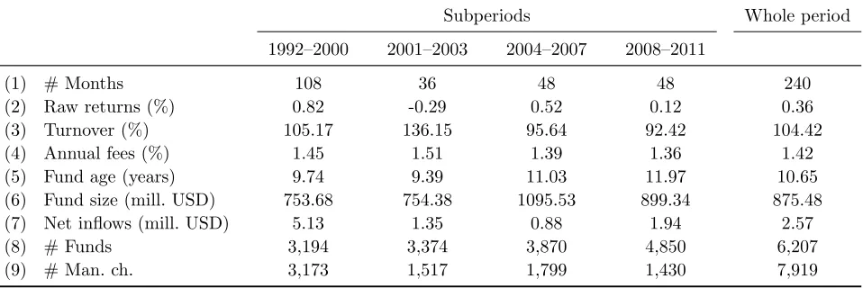
Our mutual fund sample from the Center for Research in Security Prices (CRSP) starts in 1992,

the first year for which reliable information on manager changes becomes available, and ends in

2011. We follow Pastor and Stambaugh (2002) and select only actively managed U.S. domestic

equity funds (see Table XIV in the Appendix). We aggregate all share classes of the same fund

and drop all observations prior to the initial public offer (IPO) date given by CRSP as well as

funds without names to account for a potential incubation bias (Evans, 2010). Our final sample

consists of 6,207 funds that existed at some time during the period from 1992 to 2011 for at

least 12 consecutive months. These funds have an average fund size of 875 million USD

(Table I). Fund size increased over the sample period, whereas average fees fell from 1.45

percent to 1.36 percent of assets under management.8

[Please insert Table I about here]

Monthly fund flows are constructed from the change in total net assets adjusted for internal

growth from investment returns:

1 (1)

7 _{Persistence is, however, likely to decline over time due to the operation of what we call “natural mean reversion”,}

discussed in detail in section 6.4.

8 _{Fees are calculated as the sum of the annual expense ratio and 1/7}th _{of the sum of the front end and back end loads.}

12

where TNAit refers to the total net assets of fund i at the end of period t and Rit is the return of

fund i between t-1 and t, assuming that all distributions are reinvested and are net of fund

expenses. On average, each fund received 2.57 million USD net inflows per month.

To obtain information on manager changes, we focus on the variable “mgr_date” in the

CRSP database, instead of using the specific names of the managers.9 This variable provides the

date of the last manager change as reported by the fund management company. By using the

manager date variable, we avoid any problems associated with different spellings of manager

names. Furthermore, as the number of team-managed funds increased during recent years, the

manager date variable has the advantage that companies only report significant changes in

manager/management team that are likely to have an impact on performance (Massa et al.,

2010). A total of 7,919 manager changes occurred during our sample period, which means that,

on average, 15 percent of the fund managers are replaced each year.

4.2. RESEARCH METHODOLOGY

We use ranked portfolio tests (Carhart, 1997, Carpenter and Lynch, 1999, and Tonks, 2005) to

investigate the hypotheses outlined in Section 3.

Funds are first ranked into equal-weighted decile portfolios based on their previous

performance over rolling twelve-month periods. Then, in a second sorting of the top-decile-10

and the bottom-decile-1 portfolios, we form subgroups based on fund flows (low net inflows /

high net inflows) or manager changes (with manager change / without manager change): see

9 _{This variable has also been used by Lynch and Musto (2003) and Cooper et al. (2005). In theory, it shows the date}

13

Figure 1.10 Furthermore, as we are interested in the interaction effects between both

mechanisms, we also form subgroups by double sorting on fund flows and manager changes

simultaneously (low with / low without and high with / high without). We analyze the

performance of these subgroups of top and bottom decile portfolios and the performance of

spread portfolios.

[Please insert Figure 1 about here]

The decile portfolios are formed either (a) on the basis of each fund’s alpha in the

previous year or (b) on the basis of previous-year raw returns. For the first method, funds are

ranked by alphas from a Carhart (1997) four-factor model estimated over the previous 12

months (the formation period), where the four common factors are the excess return above the

risk-free rate on the market index , the returns on a size factor , a

book-to-market factor ( , and a momentum factor ( ). Fund excess returns above the risk-free

rate accounting for different fund styles are given by:

(2)

To assess performance and fund flows in a timely manner, we focus on the previous

12-month horizon. Using such a short horizon to estimate alphas from a factor model is problematic

on account of the low degrees of freedom available for estimating (2). Nevertheless, we are able

to efficiently estimate (2) over this short horizon by applying the “empirical Bayes” adjustment

10 _{In Berk and Green (2004), active management suffers from decreasing returns to scale, but it is an empirical}

14

procedure discussed in Huij and Verbeek (2007, hereafter HV), assuming a multivariate normal

prior. Let , , , , be a vector of unknown parameters to be estimated. The

cross-sectional distribution of the funds’ alphas and betas is assumed to be normal, ~ ,Σ ,

where is a 5-dimensional vector of cross-sectional means of alphas and betas, and Σ is a 5x5

covariance matrix. Assuming the errors in (2) are distributed as ~ 0, , the posterior

distribution of is also normal with expectation:

(3)

where is the matrix of returns on the four factors plus the intercept, is the OLS parameter

estimate, and is the variance of the errors in (2). The corresponding covariance matrix is

given by:

Σ (4)

As the prior mean µ and the prior covariance matrix Σ in Equations (3) and (4), we take

the cross-sectional averages of the time series OLS estimates of the coefficients of (2) and their

corresponding empirical covariance matrix for all funds in the cross section of our sample in a

given 12-month formation period.11 Thus, we have the same priors for all funds in a given

month. According to Equation (3), the posterior estimate of is the matrix-weighted average of

the prior and the OLS estimate ; the same holds for the posterior estimate of the covariance

11 _{Specifically, we estimate time-series OLS regressions for each of the N funds in the data set for months 1 to 12.}

We average the N estimates to form µ and use the empirical covariance matrix of these N estimates to form Σ.

We plug µ and Σ into Equations (3) and (4) to obtain the mean and variance of the posterior distribution of for

15

matrix in Equation (4).12 Confidence in the prior is the reciprocal of the estimation efficiency of

the OLS estimate for each fund. Thus, the empirical Bayes adjustment “shrinks” any extreme

parameters towards the mean of the prior, where the degree of shrinkage depends on the

cross-sectional dispersion of the parameters, given by Σ. The empirical Bayes adjustment is greater,

the lower the estimation efficiency of the funds' OLS parameters. The intuition is that it is less

likely for a fund to generate high alphas if all other funds generate relatively low alphas during

the same period. However, the posterior distribution of also takes the multivariate nature of

the coefficients’ inter-relationship into account: e.g., if small-cap funds tend to have positive

alphas (i.e., there is a positive correlation between and in Equation (2)), a negative OLS

estimate of a small-cap fund i’s alpha receives a positive empirical Bayes adjustment.

This argument is similar to the methodology of Cohen et al. (2005) who, in addition, take

the similarity in investment strategies into account. They attribute a higher skill level to fund

managers who deliver their outperformance with a similar strategy to other skilled fund

managers in comparison with managers who used a completely different strategy. The latter are

classified as lucky rather than skilled. Consequently, alpha-sorting based on Bayesian

four-factor alphas accounts for a risk-adjustment of the performance measure used for the ranking,

corrects for different investment styles and reduces the influence of high-risk strategies on the

ranking. We also compare these results with portfolio formation based on raw returns, but we

12 _{HV experimented with various methods to obtain the posterior estimates, such as simple linear shrinkage,}

16

believe that, in contrast to the raw return-sorting, the Bayesian alpha-sorting provides a much

more reliable way of separating skilled from unskilled but lucky fund managers.13

5. Empirical Results

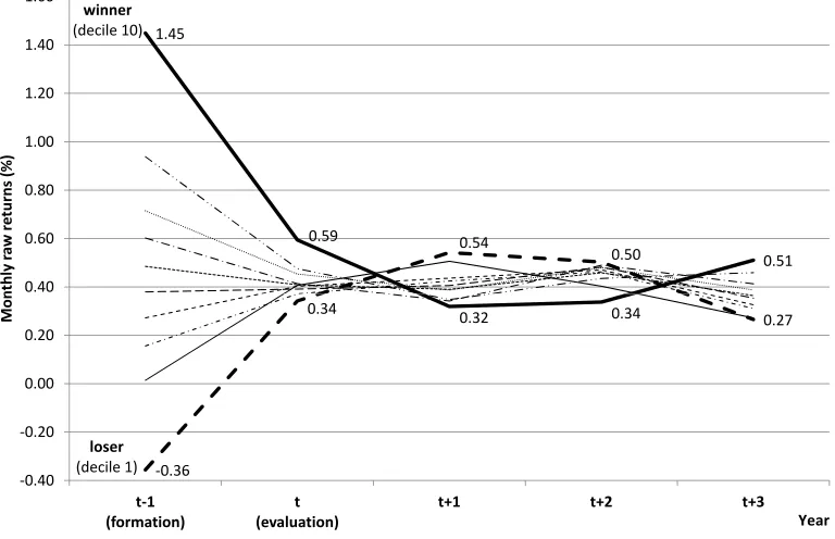
Figure 2 demonstrates that the dynamics of mutual fund returns over time are consistent with the

earlier conclusions of Carhart (1997) who reported a lack of performance persistence and a

strong tendency for performance to mean revert. Specifically, the top ten percent of funds

(winner funds)14 generate average raw returns in the formation year of 1.45 percent per month

which decline to 0.59 percent per month in the subsequent evaluation year. The bottom ten

percent of funds (loser funds), in contrast, experience a mean reversion in raw returns from

-0.36 to 0.34 percent per month. In other words, a raw return spread between winner and loser

funds of 1.81 percent per month (21.72 percent per annum) in the formation year declines to

0.25 percent per month (3.00 percent per annum) in the evaluation year. Having established that

performance persistence is mean reverting amongst both winner and loser funds, we now

investigate how fund flows and manager changes influence these results.

[Please insert Figure 2 about here]

5.1. WINNER FUNDS

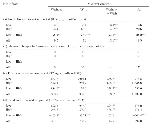
Winner funds, on average, have a formation-period fund size of 794.0 million USD and receive

8.5 million USD of new net inflows per month (Table II). They grow to an average size of

1,037.0 million USD in the evaluation period due to internal (investment performance) and

13_{The average fund flows in the deciles and subgroups are not qualitatively different when we form portfolio deciles}

based on raw returns instead of the Bayesian four-factor alphas. Since raw returns are more relevant to retail investors who are unlikely to calculate four-factor alphas, it is comforting to know that average fund flows in the deciles and subgroups are not sensitive to the sorting criteria. The subgroups should not be affected as we explicitly use fund flows as a second sorting mechanism.

17

external (fund flows) growth. Conditioning on fund flows, we separate winner funds into a

subgroup with “low absolute net inflows” during the formation period, averaging -5.6 million

USD per month, and a subgroup with “high absolute net inflows”, averaging 22.6 million USD

per month, a significant difference of 28.2 million USD. The fraction of managers leaving

winner funds is the same for both subgroups at 17 percent,15 but winner funds with low absolute

net inflows tend to be smaller (675.0 million USD) than winner funds with high absolute net

inflows (976.4 million USD).16 _{Conditioning on manager changes yields a subgroup “without}

manager change” which has slightly higher inflows (last row of panel (a)) and a larger average

fund size (last row of panel (d)) compared to the subgroup “with manager change”.

[Please insert Table II about here]

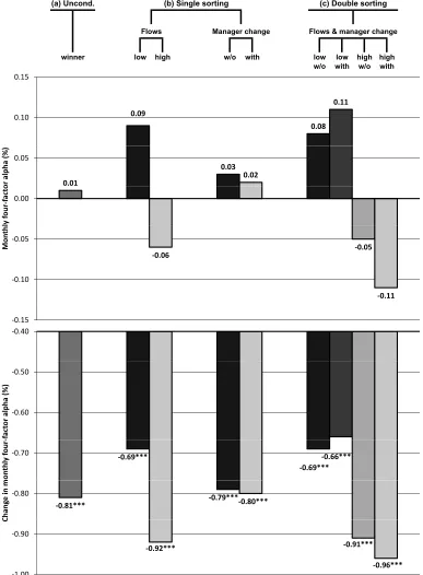
Winner-decile-10 funds, on average, generate alphas of 0.01 percent per month, equivalent to a

mean reversion from the formation to the evaluation period of -0.81 percentage points per

month (Table III, panels (a) and (c), and Figure 3). Winner funds experiencing neither high

inflows nor a manager change outperform the benchmark model (2) by an insignificant 0.08

percentage points per month. This corresponds to a significant mean reversion of -0.69

percentage points per month. Winner funds suffering from both high inflows and a manager

change generate negative, albeit insignificant, alphas of -0.11 percent per month, equivalent to a

significant mean reversion of -0.96 percentage points per month. The evaluation-period spread

in alphas of 0.19 percentage points per month between winner funds experiencing neither

15 _{This is higher than the industry average of 15 percent across the sample period (which includes funds in deciles}

2-9 as well as those in deciles 1 and 10).

16 _{According to Chen et al. (2004), differences in fund size affect fund performance. However, using relative net}

18

mechanism and those experiencing both is significant in statistical and economic terms (0.19 =

0.08 (low/ without) – (-0.11) (high/ with), Table III, panel (a)). The difference in raw returns

between winner funds suffering from both equilibrating mechanisms and those affected by

neither is also striking: raw returns of the former revert to equilibrium at a statistically

significant -1.16 percentage points per month compared with -0.62 percentage points per month

for the latter (Table IV, panel (c)). We conclude from this that fund flows and manager changes

acting together strongly contribute to mean reversion in winner-fund performance.

[Please insert Tables III and IV and Figure 3 about here]

As we have already seen in Table II, panel (b), the occurrence of a manager change

seems to be independent of fund flows, since, on average, 17 percent of managers change each

year in both subgroups with high and low net inflows. The difference in monthly fund flows

between winner funds without and those with a manager change is statistically significant but

economically small at 3.6 million USD. This suggests that the incidence of one mechanism does

not affect the likelihood of the other mechanism occurring.

Even though the mechanisms appear to operate independently of each other, controlling

for one could still alter the impact of the other on future performance, and this is what we find.

Among winner funds, there is evidence that the two mechanisms interact as complements. If

there is a manager change, high fund inflows have a significantly negative impact on

performance of 0.22 percentage points per month, whereas if there is no manager change, the

effect of high inflows is to reduce performance by only (albeit a still significant) 0.13 percentage

points per month (Table III, panel (a)). Comparing the single sort results, fund flows have a

high-19

inflow groups being a significant 0.15 percentage points per month. In contrast, a single sort on

manager change has little effect on the performance of these winner funds with only a 0.01

percentage points per month spread.

We conclude that fund flows by themselves and, especially if reinforced by a manager

change, significantly affect winner-fund performance and that fund flows and manager changes

are complementary to each other. However, high net inflows are much more harmful for

subsequent performance than a manager change, possibly as a result of the transaction costs

triggered by a liquidity-induced increase in trading. A manager change by itself has little effect.

5.2. LOSER FUNDS

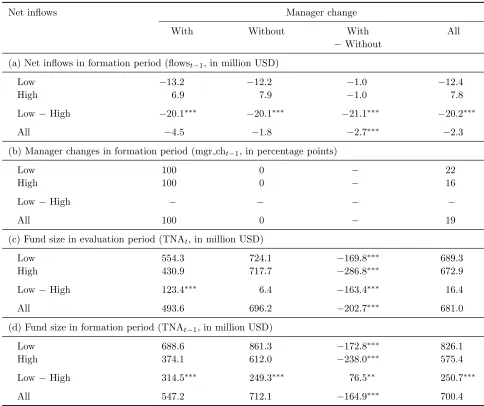
Loser funds, on average, are smaller than winner funds with total net assets of 700.4 million

USD in the formation period (Table V, panel (d)). Fund size decreases only slightly to an

average of 681.0 million USD in the evaluation period. This is explained by negative net

inflows, as expected, although these are relatively small in magnitude at only -2.3 million USD

per month, on average. The explanation is that many investors are reluctant to withdraw money

from poorly performing funds. We sort the loser-decile-1 funds into two subgroups on the basis

of net inflows, one experiencing the lowest net inflows (i.e., the largest outflows) averaging

-12.4 million USD and the other with high net inflows averaging 7.8 million USD. The

difference in average fund flows between the low- and high-fund-flow subgroups of loser funds

is only about two-thirds as large as the same difference for winner funds (20.2 versus 28.2

million USD). Loser funds with high net inflows and a manager change are the smallest

subgroup in the formation period with an average size of 374.1 million USD, while loser funds

experiencing both governance mechanisms simultaneously are the largest at 688.6 million USD

20

[Please insert Table V about here]

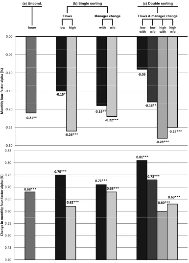
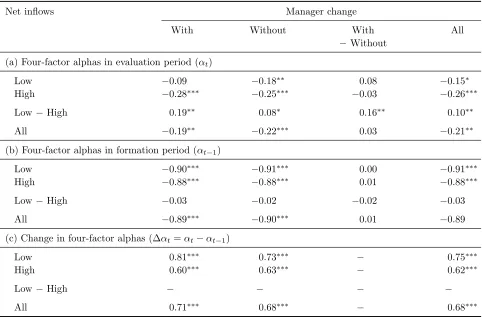
Tables VI and VII report the interactions of the two governance mechanisms and fund

performance. Loser-fund performance, on average, reverts from alphas of -0.89 percent per

month in the formation period to (a still significantly negative) -0.21 percent per month in the

evaluation period, a statistically significant performance improvement of 0.68 percentage points

per month (Table VI, and Figure 4). However, distinct differences emerge in evaluation-period

performance when conditioning on the mechanisms. Loser funds that benefit from both

mechanisms have insignificant alphas of -0.09 percent per month in the evaluation period

compared with significant alphas of -0.90 percent per month in the formation period which

corresponds to a significant and striking mean reversion of 0.81 percentage points per month.

Funds without either form of mechanism continue to significantly underperform by -0.25

percentage points per month, regressing to the mean by just 0.63 percentage points per month.

The spread in alphas between loser funds experiencing both mechanisms and those benefiting

from neither is a highly significant 0.16 percentage points per month (0.16 = -0.09 (low/ with) –

(-0.25) (high/without), Table VI, panel (a)). Differences in mean reversion based on raw returns

are even more pronounced: the raw returns of loser funds with a manager change and low net

inflows improve by a (weakly) significant 0.84 percentage points per month; while the raw

returns of loser funds without a manager change and high net inflows improve by an

insignificant 0.56 percentage points per month (Table VII, panel (c)). Thus, if operating

simultaneously, the internal and external governance mechanisms strongly contribute to an

improvement in loser-fund performance.

21

How do the mechanisms contribute to this effect? A comparison of the two subgroups

reveals that they interact positively: funds with low net inflows have a higher fraction of

manager changes (22 percent) than funds with high net inflows (16 percent),17 and funds with a

manager change have lower net inflows (-4.5 million USD per month) than funds without (-1.8

million USD per month) (Table V, panels (a) and (b)). Moreover, internal and external

governance among loser funds are also complements in terms of their performance impact. The

alpha spread between loser funds with low net inflows and those with high net inflows is

significantly positive at 0.19 percentage points per month only when internal governance is

operating at the same time. If there is no internal governance, this spread is a weakly significant

0.08 percentage points per month (Table VI, panel (a)). Conversely, the spread between loser

funds with a manager replacement and those without is positive but insignificant at 0.08

percentage points per month if money is flowing out of the fund at the same time, while it is

negative and also insignificant at -0.03 percentage points per month if outflows do not occur.

Thus, internal governance seems to be more effective if external governance is simultaneously

operating.

The results for raw returns are similar in magnitude. Outflows improve loser-fund raw

returns by a significant 0.21 percentage points per month in combination with a manager

replacement, and a positive but insignificant 0.08 percentage points per month in the case of no

manager change (Table VII, panel (a)). Compared with the similar sized alpha spread of the

same subgroup, this implies that fund managers who stay with the fund do not seem to use the

outflows to re-optimize their portfolio by bringing in new investment ideas, but merely scale

17 _{This compares with a 15 percent average turnover of managers across the industry and a 17 percent average}

22

down existing investments in a way that reduces unfavorable factor loadings in the benchmark

model. Specifically, loser funds without outflows have significantly negative momentum

loadings, while those experiencing outflows reduce these loadings to levels close to zero (not

reported in the tables).

We conclude that loser funds suffer from two types of disposition effect: one due to

investor behavior and one due to the actions of the fund management company. It appears that a

large fraction of loser-fund investors are reluctant to withdraw their money. This behavior is

consistent with a disposition effect, whereby investors are hesitant to realize losses and so stay

invested in the hope that the fund price eventually returns to the original purchase price.

However, our results also show that staying invested in loser funds is a sub-optimal strategy,

because performance remains negative. The second disposition effect relates to the reluctance of

the fund management company to fire the underperforming manager. Even when outflows

occur, as in case of the low net inflow subgroups, the performance of existing fund managers

does not respond positively to the smaller asset base. It is only when a manager change is

combined with outflows that performance significantly improves. However, outflows by

themselves have a significant effect in improving performance, although this is enhanced if the

manager is also changed.

5.3. WINNER-LOSER SPREAD

The spread in alphas between winner and loser funds for the 12-month portfolio formation

period is 1.71 percentage points per month, obtained as the difference between the unconditional

alphas in panel (b) of Table III (0.82 percent per month) and Table VI (-0.89 percent per

month). The spread in alphas between the winner and the loser funds for the 12-month

23

unconditional alphas in panel (a) of Table III (0.01 percent per month) and Table VI (-0.21

percent per month). This spread is similar to the winner-minus-loser spread in the Carhart

(1997) study, although his spread is statistically significant.

A key issue now is how this spread is affected by the equilibrating mechanisms.

Specifically, we compare the performance of the winner and loser portfolios in seven different

scenarios, which are defined in panel (a) of Table VIII. Panel (b) reports the corresponding

alphas (see also Figure 5). In the first column of panel (b), we report the alphas of funds that

experience neither mechanism. Our hypotheses suggest that we would expect to find the highest

level of positive and negative performance persistence among these funds. The next two

columns report the performance results when either the fund-flow or the manager-change

mechanism is not operating. The fourth column reports the unconditional winner-minus-loser

spread, not taking fund flows or manager changes into account. The next two columns report the

results for funds that experience one of the mechanisms. In the last column, the results where

both mechanisms operate simultaneously are reported. In this last case, we would expect to find

the strongest tendency of fund performance to revert to the mean.

[Please insert Table VIII and Figure 5 about here]

We find that winner and loser funds that experience neither mechanism yield a highly

significant winner-minus-loser spread of 0.34 percentage points per month (Table VIII, panel

(b), column (1), and Figure 5). The spread does not change for funds not experiencing high

inflows (column (2)). The spread falls to an insignificant 0.25 percentage points per month when

conditioning on funds not experiencing a manager change (column (3)). For the unconditional

24

points per month as noted above (column (4)). This spread decreases further – when

concentrating only on funds that experience either the manager-change mechanism or the

fund-flow mechanism – to an insignificant 0.20 and 0.09 percentage points per month, respectively

(columns (5) and (6)). For winner and loser funds that experience both equilibrating

mechanisms simultaneously, we find an insignificant spread between winner and loser funds of

-0.02 percentage points per month (column (7)). Thus, when investors and managers take

advantage of outperformance or investors and the fund management company react to

underperformance in the formation period, the equilibrating processes force the spread between

previous winner and loser funds to become virtually zero (-0.02 percentage points per month) in

the evaluation period. In contrast, if funds are not exposed to these mechanisms, the spread is a

significant 0.34 percentage points per month. The equilibrating mechanisms seem to be able to

explain the reduction in the winner-minus-loser spread by 0.36 percentage points per month.

This highlights the importance of fund flows and manager changes in explaining mean

reversion in mutual fund performance and why mutual fund performance is unlikely to persist in

well-functioning markets. The table also reconfirms both the dominance of fund flows (cf. the

difference between columns (5) and (6)) and the strong supporting role of manager changes

when the fund-flow mechanism is also operating (cf. the difference between columns (6) and

(7)).

6. Robustness tests

In this section, we document that these results are robust to a number of different tests.

6.1. THE EFFECT OF DIFFERENT FACTOR MODELS

We applied alternative five-factor models to investigate whether the results differed from those

25

factor (based on six value-weighted portfolios formed on the size and prior returns of all NYSE,

AMEX and NASDAQ stocks18_{) to the standard model: if winner funds hold on to winner stocks}

for another one or two years, these winner stocks might eventually experience mean reversion in

returns (De Bondt and Thaler, 1985, 1987). In the second model, we included a liquidity-factor19

to the standard model on the grounds that fund flows may also affect portfolio liquidity. We do

not present the results using these models, but can confirm that they are qualitatively similar to

those using (2).

6.2. THE EFFECT OF INTRODUCING PEER-GROUP BENCHMARKS

We adjusted for peer-group benchmarks, since these are widely used by practitioners for

evaluation purposes. We used two alternative approaches.

In the first approach, we define the peer-group-adjusted returns as the difference between

the fund’s returns and the average returns of all peer-group funds with the same fund style. We

classified the funds in our sample into 13 styles: large-cap, mid-cap, small-cap, growth, growth

& income (G&I), income, sector funds (financial, health, natural resources, technology, utilities,

other), and other. The results from evaluating performance from a ranking based on these

peer-adjusted benchmark returns are presented in Table IX for both winner and loser subgroups.

Compared with the results for raw returns, the low-minus-high row is generally lower and the

without-minus-with column is generally higher, but otherwise of similar order of magnitude (cf

Table IX with panel (a) of Tables IV and VII). The only exception is for the returns of winner

funds with a manager change but low net inflows which are significantly lower: the

corresponding low-minus-high spread is no longer significant for this subgroup. The fact that

18 _{Downloaded from Kenneth French’s website:}

mba.tuck.dartmouth.edu/pages/faculty/ken.french/data_library.html

26

the low-minus-high row is generally lower suggests that investors also respond to peer-group

differences in the performance of fund managers (in addition to differences in alphas) and this

contributes to the effectiveness of the fund-flow mechanism.

[Please insert Table IX about here]

The second approach that we adopted was to estimate the model recently suggested by

Hunter et al. (2014) which adds an active peer benchmark (APB) to the four-factor model to

control for the fact that estimation errors are potentially not independently distributed in the

cross section of funds. Adding an APB can help to account for dynamically changing

“commonalities” across fund returns (as a result of the funds following similar investment

strategies) and to improve the estimation of the prior covariance matrix (see also Pastor and

Stambaugh, 2002). Hunter et al. (2014) show that the APB can explain a significant proportion

of the cross correlation between the residuals in the four-factor model for the different funds. In

particular, they show that the within-group (individual fund pair) residual correlations are

decreased by one-third to one-half of their prior levels, depending on the peer group. This

indicates that the APB successfully captures common idiosyncratic risk-taking within peer

groups. The APB for each peer-group was estimated as the residual series from a regression of

an equal-weighted portfolio of all funds with the same investment style on the standard four

factors in Equation (2). We used the same 13 investment styles as for the peer-group-adjusted

returns listed above.

Table X reports the performance evaluation results from ranking funds on the basis of

this APB adjustment, and these results can be compared with the performance results from the

27

APB for ranking on past performance. For winner funds, the alphas in panel (a) of Table X are

in general similar to those in panel (a) of Table III. There is again one exception: winner funds

with a manager change but low net inflows now significantly outperform the extended

benchmark model (2) by 0.23 percentage points per month (without the APB adjustment, the

outperformance was an insignificant 0.11 percentage points per month). The results for loser

funds are quantitatively very similar, comparing panel (b) of Table X with panel (a) of Table VI.

Overall, the addition of various peer-group benchmarks does not change the qualitative

findings from the standard four-factor model.

[Please insert Table X about here]

6.3. A ROBUSTNESS TEST OF THE EMPIRICAL BAYES APPROACH

In an unreported test, we addressed a concern that, in our empirical Bayes approach, the prior

and conditioning information are potentially not independent because the prior is the

cross-sectional mean ( of all the funds in the sample which includes the fund i under consideration. This could potentially bias our results if fund i is an outlier. We therefore re-estimated the model

using the cross-sectional median rather than the mean as the prior to reduce the effect of any

outliers. However, this did not significantly affect our results: monthly alphas only change by

1-2 basis points and, in a very few cases, by 3 basis points.

6.4. TESTING A COROLLARY TO OUR KEY HYPOTHESIS

The key hypothesis in this paper is that if one or both of the equilibrating mechanisms are

operating, then performance will not persist: there will be mean reversion which will be

measured by the decline in alpha between the formation and evaluation periods. A corollary is

that if performance does persist and neither mechanism is operating effectively, then other

28

persistence. To assess this, we formed sub-samples of funds that are matched on the basis of six

key characteristics for which data are available: fund size, fund age, investment style, size of

distribution fees, fund family size, and investor type.

6.4.1 Winner Funds  

We begin with Table XI which looks at the effect of these characteristics on the performance

persistence of winner funds. Consistent with the evidence in Table III, panel (g) of Table XI

shows that, across the full sample, the decline in alpha between the formation and evaluation

periods (Δα ) averages -0.81 percentage points per month. However, the full sample includes

around 600 sector-specific funds and funds with other investment styles whose behavior is

unrepresentative of our overall results. When these funds are excluded, the decline in alpha

between the formation and evaluation periods averages -0.76 percentage points (last row of

panel (c)). Looking down the Δα column, winner funds appear to revert to the mean between

the formation and evaluation periods by, in general, between -0.70 and -0.93 percentage points.

We argue that the lower end of this range, between -0.70 and -0.75 percentage points, measures

what might be called the level of “natural mean reversion”. This is the mean reversion that takes

place independently of the operation of the equilibrium mechanisms as a consequence of the

luck of fund managers running out – most fund managers find themselves in the top decile of

performance due to good luck.20 Natural mean reversion might not, however, completely

eliminate performance persistence. If there is any additional mean reversion, we put this down

to the operation of the equilibrating mechanisms. If, on the other hand, the mean reversion is

less,21 then we can conclude that neither natural mean reversion nor the two mechanisms are

20 _{See Blake et al. (2014; 2017, forthcoming).}

29

working effectively and, as a consequence, performance will persist – at least over the 12 month

horizon. We examine the six characteristics in turn.

(1) Fund size.22 Panel (a) shows that Δα lies in the zone of natural mean reversion for

both large and small funds. The last three columns indicate that the two mechanisms have no

statistically significant effect, although the manager change mechanism has a little more power

in economic terms in small funds than large funds, especially when combined with fund flows.

(2) Fund age.23 Panel (b) shows that Δα lies in the natural mean reversion zone for old

funds, but it is larger in absolute terms for young funds. The last three columns reveal that the

fund-flow mechanism is highly effective in young funds, especially when combined with a

manager change. Funds flows also have some effect (albeit a statistically weaker one) in old

funds.

(3) Investment style. Most funds in the sample are either size or growth-versus-income

oriented. The final row of panel (c) indicates that, when sector-specific funds and funds with

other investment styles are excluded, Δα lies just inside the range where the equilibrating

mechanisms begin to become effective; the last three columns show that both mechanisms are

indeed working well, especially in combination.

Turning to the individual investment styles, we can see that both mechanisms are highly

successful in removing the persistence in small-cap funds – which is a very intuitive finding,

since such funds will have difficulties in managing flows for liquidity reasons. But the

mechanisms do not work in growth funds, since Δα = -0.70 is already in the natural mean

reversion zone. The mechanisms are less effective in large- and mid-cap funds, despite having a

22 _{Large (small) funds are those with above (below) median size. Chen et al. (2004) and Cremers and Petajisto}

(2009) find a negative effect of fund size on performance.

23

30

very large (in absolute terms) Δα of -0.93. This is also an intuitive result, since it is difficult for

fund managers trading in S&P500 stocks with deep and liquid markets to identify systematically

mispriced securities. Winner fund managers focusing on these investment styles are more likely

to be winners because of luck. The table shows that their luck disappears without any additional

support from the two mechanisms.

G&I and income funds are an outlier, with a Δα of just -0.36 after 12 months,

suggesting that mean reversion has not been completely achieved within this time frame. We

examined this sub-sample in further detail and looked at 24- and 36-month formation and

evaluation periods. We found that the equilibrating mechanisms – particularly, the fund-flow

mechanism – take longer to work (between two and three years).24

(4) Size of the distribution fee.25 This affects the strength of a fund’s distribution

network. Panel (d) shows that the results are similar whether the distribution fee is high or low.

In both cases, the size of Δα suggests that at least one of the mechanisms will be effective, and

the last three columns confirm that it is the fund-flow effect.

(5) Fund family size.26 The size of Δα in panel (e) suggests that at least one of the

mechanisms is effective whether the fund family is large or small. The fund-flow mechanism is

particularly effective in small fund families, especially in conjunction with a manager change. It

is reasonable to conjecture that large fund families are more able to handle strong inflows and

24 _{Carhart (1997, Figure 2) showed that the top and bottom decile funds can take up to four years for the persistence}

to be eliminated in his 1962-1993 data set.

25_{High (low) distribution fees are those above (below) the median distribution fee. Distribution fees comprise the}

front-end load (as the majority of this is usually paid to a distribution partner) plus 12B-1 fees (annual marketing fees, generally between 0.25 and 1.00% (the maximum allowed) of a fund's net assets, named after a section of the Investment Company Act of 1940). Carhart (1997) documents a negative effect from fees on net performance.

31

situations where the manager is leaving than small fund families. So the equilibrating

mechanisms should be weaker for larger fund families, which is what we find.

(6) Investor type. Panel (f) shows that with institutional funds, the size of Δα indicates

that natural mean reversion will remove any persistence without the need for the equilibrating

mechanisms. In the case of retail funds, fund flows, especially if reinforced by a manager

change make a significant contribution to mean reversion. This confirms the well-known finding

that retail investors react more strongly (and more irrationally) to good past performance than

institutional investors (Del Gurcio and Tkac, 2002).

[Please insert Table XI about here]

6.4.2 Loser Funds 

We now turn to Table XII which examines the effects of the same characteristics on the

performance persistence of loser funds. If we again exclude the unrepresentative sector-specific

and other investment-style funds, the increase in alpha between the formation and evaluation

period averages 0.64 percentage points per month (last row of panel (c)). The Δα column

shows that loser funds appear to revert to the mean between the formation and evaluation

periods by, in general, between 0.59 and 0.75 percentage points, which is lower both in absolute

terms and in range than is the case with winner funds. We will again argue that the lower end of

this range, say, between 0.59 and 0.63 percentage points, measures the level of natural mean

reversion for loser funds – reflecting the fact that many loser fund managers find themselves in

the bottom performance decile due to bad luck. It follows that any additional mean reversion is

due to the operation of the equilibrating mechanisms, while a lower degree of mean reversion

implies that the mechanisms are not working over the 12 month horizon. We again examine the

32

(1) Fund size. Panel (a) shows that, for large funds, Δα = 0.63 which is within the zone

where natural mean reversion operates. This is confirmed by the last three columns which show

that the two mechanisms are not working. However, for small funds, Δα at 0.75 is much higher

and this is explained by investors taking money out of these funds.

(2) Fund age. Panel (b) reveals that both mechanisms are highly effective in removing

persistence in old funds, but are completely ineffective in the case of young funds, despite the

fact that Δα is similar for both types of funds. It is also interesting to note that it is only in the

case of old funds that the manager-change mechanism is effective by itself (see the single

sorting with-minus-without column). This appears to suggest that investors are prepared to give

the managers of new loser funds a chance to rectify their poor performance, but not those in

established funds.

(3) Investment style. The final row of panel (c) shows that the fund-flow mechanism is

effective on average across all investment styles.27 Digging down more deeply, we observe that

this mechanism is particularly effective with small-cap funds, and also with growth, large- and

mid-cap funds if accompanied by a manager change. However, as with the case of winner funds,

the mechanisms do not work in G&I and income funds over a one-year horizon (the Δα is only

0.44). Looking at 24- and 36-month formation and evaluation periods for these investment

styles, we find that there is still some residual persistence even after three years, despite the fact

that the manager-change mechanism has some effect over the 24 month horizon. A possible

explanation for funds with G&I and income investment styles being outliers for both winner and

loser portfolios is an investor clientele effect. These funds are primarily held by investors

interested in their long-term income-generating capabilities and are eschewed by other types of

33

investor, e.g., those more interested in growth than income. Income-seeking investors will be

prepared to hold on to loser funds, while growth-seeking investors will not rush into winner

funds, preferring instead to look for more attractive opportunities in other sectors.

(4) Size of the distribution fee. Panel (d) shows that in terms of distribution fees, despite

having virtually the same Δα , there is a powerful fund-flow effect in the case of funds with low

distribution fees, but not in the case of funds with high distribution fees. The latter appear to be

able to restrict outflows using a strong distribution network, thereby hindering the equilibrating

mechanism.

(5) Fund family size. In contrast with the case for winner funds, fund flows are more

effective in restoring equilibrium in the loser funds of large fund families than those of small

families, especially when combined with a manager change (panel (e)).28 Further, the internal

governance mechanism is very weak, particularly in the case of small families: the latter might

be owner-managed and the owner is unlikely to sack herself.

(6) Investor type. Panel (f) shows that the results are similar to the case of winner funds.

Natural mean reversion removes the persistence in institutional funds without the need for the

equilibrating mechanisms. In the case of retail funds, fund outflows, especially if reinforced by a

manager change, make a significant contribution to mean reversion, although it is weaker than

in the case of winner funds. This is perhaps a little surprising, given the well documented

evidence that retail customers are prone to a disposition effect.

[Please insert Table XII about here]

28 _{This finding supports the predictions of Gervais et al. (2005) that a manager replacement in a large family}

34

6.4.3 Comment 

The robustness tests in this section provide broad support for the key hypothesis of this paper:

performance persists unless either the two equilibrating mechanisms or natural mean reversion

operate to remove it. However, this needs to be qualified as follows. The mechanisms do not

appear to work for loser G&I and income funds over a one-year horizon: in the case of winner

funds with these investment styles, for example, it takes two years rather than one for the

persistence to be eliminated.

A further implication is that we do not find any other unobserved characteristic

explaining the persistence spread. Our sorting procedure explains how we reach this conclusion.

We re-form all portfolios every year based on the previous year’s performance. So, over the

course of the full sample, individual funds move between the sub-portfolios (e.g., from winner

to loser, from low to high flow, from without to with manager change, and vice versa). If the

portfolios were established once at the beginning of the sample period, then it might be possible

that another unidentified characteristic could explain the performance spread we observe. But

with the continuous re-forming of portfolios, each fund will move across many different

sub-portfolios over the 20 years of our sample period. Hence, even if there is some unobserved

characteristic, a fund with a specific embodiment of that characteristic would move between

many different sub-portfolios over time and, thus, the characteristic is unlikely to play a

significant role in explaining our findings.

6.5. CONTROLLING FOR DIFFERENT MARKET CONDITIONS

Glode et al. (2012) extend the Berk-Green framework to examine the issue of whether the way

that investors respond to past performance through fund flows helps to identify predictability in

mutual fund returns. They find that there is predictability in mutual fund returns and that it is

35

market returns, but not after periods of low market returns. They find no persistence in

under-performing funds, irrespective of market conditions.

We adapt this analysis of time-varying persistence to examine the strength of the

equilibrating mechanisms that we have identified, controlling for market conditions. Glode et al.

(2012) identify up-markets and down-markets using excess market returns on a quarterly basis.

Our data set does not allow us to conduct such a high-frequency analysis. Instead, we identify

four sub-periods within the full sample from 1992 to 2011: 1992 to 2000 (bull market), 2001 to

2003 (bear market), 2004 to 2007 (bull market) and 2008 to 2011 (bear market). Within each

sub-period, we calculate both the degree of persistence in mutual fund performance and the

alpha spreads on the basis of single and double sorts by fund flows and manager changes.

The first column of panel (a) of Table XIII shows that there is little evidence of

persistence (as measured by the evaluation period alpha) for the winner funds, irrespective of

market conditions. The Δα column indicates wide variation in the decline in alpha across the

four sub-periods and there is insufficient information to determine the level of natural mean

reversion, although it too is likely to differ widely across the sub-periods. Nevertheless, in most

sub-periods, the persistence is removed by the operation of the fund-flow mechanism, if only

weakly during the 2001-2003 bear market (column 4).

There is, however, persistence for loser funds in both bear markets of 2001-2003 and

2008-2011, despite, in the latter case, fund flows operating much more effectively than in the

earlier bear market (panel (b)). This confirms findings first made by Carhart (1997) that there is

some persistence in the worst performing loser funds. Carhart did not separate his 1962-1993

data set into bull and bear sub-periods, but our findings would appear to suggest that any

36

The only occasion in which manager changes had a statistically significant effect in eliminating

persistence was in loser funds in the 1992-2000 bull market (column 6).

[Please insert Table XIII about here]

7. Conclusions and Implications

We have examined the effects of fund flows and manager changes as equilibrating mechanisms

in explaining the removal of persistence in mutual fund performance over time. Using a CRSP

sample of 6,207 actively managed U.S. equity mutual funds over the period from 1992 to 2011,

we find that a significant part of the mean reversion in both winner and loser funds is explained

by the two mechanisms operating together, i.e., by the responses of investors, fund managers

and fund management companies to past performance.

We have found that winner funds with high inflows experience a deterioration in

subsequent performance. This effect is much more important in explaining below-average

performance than, say, the impact of fees. We therefore provide empirical support for the Berk

and Green (2004) hypothesis that inflows of new money contribute significantly to mean

reversion. We also found that winner funds with a manager change suffer from a deterioration in

subsequent performance, but the effect is very small compared with the impact of fund flows.

Further, winner funds where both mechanisms operating simultaneously experience an

amplified effect on future performance, confirming that the mechanisms are complements.

With respect to loser funds, we found funds with high outflows enjoyed an improvement

in subsequent performance. For loser funds with a manager change, we observe improved

subsequent performance, but again the effect is very small compared with the impact of fund