SAR image segmentation with GMMs

City, University of London Institutional Repository

Citation

:

Belloni, C., Aouf, N. ORCID: 0000-0001-9291-4077, Merlet, T. and Le Caillec, J.

(2017). SAR image segmentation with GMMs. In: International Conference on Radar

Systems (Radar 2017). . London, UK: IET. ISBN 978-1-78561-672-3

This is the accepted version of the paper.

This version of the publication may differ from the final published

version.

Permanent repository link:

http://openaccess.city.ac.uk/22090/

Link to published version

:

Copyright and reuse:

City Research Online aims to make research

outputs of City, University of London available to a wider audience.

Copyright and Moral Rights remain with the author(s) and/or copyright

holders. URLs from City Research Online may be freely distributed and

linked to.

City Research Online:

http://openaccess.city.ac.uk/

publications@city.ac.uk

SAR Image Segmentation with GMMs

Carole Belloni

, Nabil Aouf

, Thomas Merlet

, Jean-Marc Le Caillec

∗_{Cranfield University, Signals and Autonomy Group, Defence Academy of the UK, c.d.belloni@cranfield.ac.uk,} †_{Thales Optronique, Elancourt, France,}§_{IMT Atlantique, Brest, France.}

Keywords: SAR, MSTAR, GMM, Segmentation

Abstract

This paper proposes a new approach for Synthetic Aperture Radar (SAR) image segmentation. Segmenting SAR images can be challenging because of the blurry edges and the high speckle. The segmentation proposed is based on a machine learning technique. Gaussian Mixture Models (GMMs) were already used to segment images in the visual field and are here adapted to work with single channel SAR images. The seg-mentation suggested is designed to be a first step towards fea-ture and model based classification. The recall rate is the most important as the goal is to retain most target’s features. A high recall rate of 88%, higher than for other segmentation methods on the Moving and Stationary Target Acquisition and Recog-nition (MSTAR) dataset, was obtained. The next classification stage is thus not affected by a lack of information while its computation load drops. With this method, the inclusion of disruptive features in models of targets is limited, providing computationally lighter models and a speed up in further clas-sification as the narrower segmented areas foster convergence of models and provide refined features to compare. This seg-mentation method is hence an asset to template, feature and model based classification methods. Besides this method, a comparison between variants of the GMMs segmentation and a classical segmentation is provided.

1

Introduction

The purpose of segmentation is to give meaning to an image and facilitate further analysis. In the particular case of the MSTAR dataset, two types of segmentation are observed. The segmentation can focus on the target only or on both the tar-get and its shadow. It is challenging to segment SAR images, as there are no sharp edges to delimit the target or the shadow from the background. The presence of noise with a high stan-dard deviation makes the choice of a direct threshold diffi-cult as either the target will not be entirely detected, or some background will be falsely detected. Most of the segmenta-tion methods already implemented try to isolate the target only [1] [2]. After going through some pre-processing, the segmen-tation is done using thresholds. Some methods [3] enhance the precision of the method by applying an adapted threshold based on the contour of the previously found target. It is hard to evaluate and compare the segmentation results as there is no publicly available official ground truth. One manual

seg-mentation method was proposed as a segseg-mentation reference. It includes manual segmentation by an analyst followed by a quality control check by a supervisor [4]. However, the re-sult of this segmentation is not publicly available and would be labour intensive to reproduce. Another ground truth was proposed by simulating the projection of the 3D CAD target’s model on the ground in a similar configuration to the MSTAR dataset to estimate the contour of both target and shadow [5]. This is what we will use to evaluate the proposed segmentation method. To our knowledge, no existing paper gives the com-plete set of precision, recall and dice score with this ground truth.

Unlike previous methods where the focus was on achieving a good segmentation by the usual standards such as a high Dice score, the main objective here is to ease the classification pro-cess. The objective is to retain all possible features from the target while discarding the noise. This improves all types of classification methods. Indeed, the templates are lighter, the comparison of features is faster with refined features and the convergence of models is boosted with noise reduction. This segmentation can also prevent mismatches between features of the target and the clutter as it will be suppressed through seg-mentation. The main evaluation of our method will be through the recall rate, while providing the other classical rates, to as-sess the retention of the target area. However, the area around the target can be misclassified as the target because of the recall rate focus. This is balanced by the additional information the multipath near the target can give. This segmentation fulfills its purpose if the classification does not rely on shape recog-nition. We made this assumption as we believe that contour shapes do not strongly characterise SAR targets.

Firstly the SAR database and segmentation ground truth used to evaluate the method are presented. The whole segmentation process is then described, explaining the acquisition of a back-ground GMM model and the actual process of GMM segmen-tation. Finally a comparison between different segmentation techniques is given.

2

Dataset

2.1 MSTAR dataset

(Horizon-Initialization

Evolution

Actual segmentation

target chips Initializationof the GMM Background_model

New types of background

Segmented image Morphological

Processing Target

chips Pre-processing

Pre-processing

Distance image

Compare the background model with the new image

Thresholding

(a)

(b)

(a)

(c)

(d)

(f)

(e)

Fig. 1:Pipeline of the segmentation process

tal Horizontal) polarisation in X-Band. There are nine targets. The low resolution and blurred edges make it a challenge to get a precise segmentation.

2.2 Segmentation ground truth

The segmentation ground truth used for our method’s evalua-tion is based on the findings of [5]. The 3D CAD model of the target is orthographically projected with the same orientation displayed in the image. The result is a 2D segmented image. The exact position of the segmented objects is adjusted to best fit the images using a correlation criterion. There are 33 se-quences available and segmented with this method out of the 44 sequences of the MSTAR dataset from different targets and different depression angles. All 33 will be used to evaluate the segmentation results of the presented method.

3

Technical description of the segmentation

The presented segmentation method relies on the GMM ma-chine learning technique. The major steps of the method can be seen in Fig.1. Firstly, the initialisation (in green in Fig.1) gets a model of the background. To initialise the background GMM model, a few target chips are chosen and processed to extract a GMM characterisation of the background. Then, the actual segmentation (in blue in Fig.1) can be done by comparing the background model to the image to segment. This gives a dis-tance image representing the likelihood of the area to belong to the background. The final image is obtained after thresholding the distance image and some further morphological process-ing. The remaining areas are the ones the least likely to be part of the background, namely the target in the foreground. The algorithm can work without evolution (in yellow in Fig.1), however adding a learning phase makes it more accurate as the background is not the same throughout each sequence. The background model integrates new types of background as well as discarding the GMMs not representative any more of the current background along the sequence of images.

3.1 Choice of the initialising target chips

The first step consists in choosing the images that will be used to initialise the background. We choose few images from the beginning of the sequence rather than along each sequence. The variety of GMMs fitting the background at each stage is achieved along the sequence by making the model evolve.

3.2 Data pre-processing

Different pre-processing were tested in order to obtain the best segmentation. The objective of the pre-processing, (a) in Fig.1, is to reduce the noise without blurring the contour of the tar-get. The choice of the pre-processing method was done em-pirically. The GMM segmentation was applied after the dif-ferent pre-processing methods on the images where the classi-cal segmentation methods failed the most, mostly because of a change of background. We evaluated the segmentation on the recall rate and dice score of the specification on those images. Two bilateral filters and a median filter is the combination that gives the best results. This pre-processing was compared with other pre-processing methods such as mean filtering, contrast stretching or histogram equalisation.

3.3 Adaptation of the GMM to the single channel SAR image

The GMM is a probabilistic model made from a combination of Gaussians to represent data that could be subdivided in dif-ferent subsets. It has already been used to segment visual im-ages [7]. In our case, the GMMs represent different areas of the images and follows Eq.1. The background is modelled instead of the target as it has less variance and is more predictable.

 



B(θ1, ..., θn) ={GM M1(θ1), ..., GM Mn(θn)}

GMMi(θi) = K

P

j=1

φj∗ Nj (1)

whereBis the background model, GM Mi is theithGMM

composing the background model. Each GMM is made of K GaussiansNjwith a weightφjover an observed intensity

dis-tributionθj.

Start-(a)Original image (b)Distance image

Fig. 2:Distance image between the extracted GMMs and background model

ing directly by expectation-maximisation (EM) is likely to fall in a local minima. The EM gets a more accurate estimation of the GMM parameters. As the background occupies the most space in the images, the GMMs related to the background are the most frequent ones. The most similar GMMs are grouped together to determine their prevalence. The similarity is estab-lished using the Kullback-Leibler (K-L) divergence based on Gaussian approximation [8] written in Eq.2.

 



dist(GM Mi, GM Mj) = min

∀m∈Si,∀n∈Sj

KL(Nm,Nn)

KL(Nm,Nn) = ln

σn

σm

+(µm−µn)2+σ2m−σ2n 2σn

(2) whereSiis the number of Gaussians in theGM Mi,Nmis the

mthGaussian distributionN(µm, σm)of theGM Mi.

If the divergence is below a threshold, the GMMs are con-sidered similar and the weight representing the occurrence of these GMMs is updated as the sum of the two GMMs weights. The GMMs selected to model the background are the 80% GMMs with the heaviest weight. They are likely to represent the background as one target only occupies around 2% of the image space in the MSTAR dataset.

3.4 Segmentation

The segmentation is a two phases process. The distance image, (c) in Fig.1, is computed using the background model previ-ously obtained and the new image. It is then thresholded, (d) in Fig.1, to obtain the binary segmented image.

3.4.1 Distance image

The image is divided in 10×10 square patches and a GMM is deduced from each patch. The distance image in Fig.2 links the pixels’ intensity to the K-L divergence as in Eq.2 between the GMMs from the background model and the GMMs found in the image to segment. Each patch’s new intensity is the min-imal divergence found between the new GMM and the back-ground model GMMs. A logarithmic filter stretches the lower intensities and makes the choice of the threshold more accu-rate.

3.4.2 Thresholding

The choice of the threshold (d) in Fig.2 relies on the assump-tion that the target covers a small part of the image. The thresh-old is chosen so that only the brightest part of the image is retained. A larger threshold could be used as the post mor-phological processing would suppress the majority of the false alarms but some false alarms could still remain.

(a)Original image (b)Segmentation result

Fig. 3:Result of the segmentation without evolution

(a)GMM candi-dates

(b)Segmentation with evolution

Fig. 4:Location of the GMM candidates and result of the seg-mentation with evolution

3.5 Morphological filtering

Morphological filtering, (e) in Fig.2, is essential to correct the first results of the segmentation. The target can be split up after the segmentation process in different parts and the dila-tion helps reconnecting them. However, the diladila-tion makes the detected target larger and swells the misclassified background parts. The dilation is thus followed by an erosion. At this stage, the target is detected and its shape is well approximated but there are still false positives. Most are removed while ar-eas below a specific surface are suppressed. An optional step is to add a dilation boosting the recall rate. As the target is now the only positive area, a dilation adds to the detection areas surrounding or on the target.

3.6 Evolution of the background model

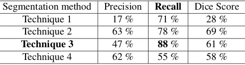
Segmentation method Precision Recall Dice Score Technique 1 17 % 71 % 28 % Technique 2 63 % 78 % 69 %

Technique 3 47 % 88% 61 % Technique 4 62 % 55 % 58 %

Table 1:Segmentation results: Technique 1: Basic GMMs. Technique 2: GMMs with evolution. Technique 3: GMMs with evolution and morphological processing. Technique 4: Pre-processing and thresholding [9].

improvement on the result of the segmentation by comparing Fig.3b and Fig.4b to the original shown in Fig.3a.

4

Results

The main objective of this segmentation is to detect the target as a whole even if the precision decreases. False negatives are more damaging for further processing and classification than false positives. Indeed, the clutter having none of the target features will be discarded at the classification stage whereas a part of the target missing could mean the loss of a crucial fea-ture. This is why the recall rate is used as the important crite-rion to evaluate the performance of our segmentation method.

4.1 GMM technique

The very low rate of 17% of precision of technique 1 in Table 1 shows that the basic GMMs technique is prone to false alarms. This endorses the overall change of the background through-out the sequences and that the background model should be updated accordingly. This hypothesis is confirmed looking at the 63% precision rate achieved once the evolution process is introduced as per technique 2. The number of true positives increases with the recall rate. There can be more true positives because of the dilation only if the previously detected area is al-ready on or near the target. The difference between the recalls of techniques 2 and 3 from 78% to 88% in Table 1 confirms the previous detection was rightly located. As can be seen in Table 1 from the precision and recall rate of techniques 2 and 3, the last morphological step is a trade-off between precision and recall. With the highest recall rate, technique 3 is favoured.

4.2 Comparison with other techniques

Technique 4 in Table 1 is used as a preliminary step to sev-eral classification methods [9] [2]. This method consists of an histogram equalisation followed by a mean filter as prepro-cessing. A constant intensity threshold is then used to remove the pixels with a low intensity. The median of the intensity of the pixels remaining is used as a second threshold. Usually the target is well detected even if it is in several pieces. However, the background is detected as well. These results are shown by a comparable precision of the GMM technique 2 of 62% seen in Table 1 but a much lower recall rate of 55%.

5

Conclusion and future work

The presented technique has a high recall rate of 88% satis-fying the objective of a loose segmentation keeping most of

the target and its features while removing the background to ease further analysis of the image. We observed a higher recall rate for this segmentation method than for other techniques that we tested. This can be interesting for feature or model based classification methods with a heavy computation load but that requires a detailed description of the target. Further work is considering several processes to increase the precision of our algorithm. The dilation could be done with a kernel whose size varies with the probability of the area to contain a target us-ing the distance image. A fine edge detection could be added around the border previously found with the segmentation to get a more accurate contour of the target. The segmentation could also be extended to detect both the target and its shadow. Either the threshold method could be changed to cluster the histogram in three classes or a shadow model could be created as the presented background model.

References

[1] M. Amoon and G.-A. Rezai-Rad, “Automatic target recognition of synthetic aperture radar (SAR) images based on optimal selection of Zernike moments features,” IET Computer Vision, vol. 8, no. 2, pp. 77–85, 2013. [2] A. Agrawal, P. Mangalraj, and M. A. Bisherwal, “Target

detection in SAR images using SIFT,” inSignal Process-ing and Information Technology (ISSPIT), 2015 IEEE In-ternational Symposium on. IEEE, 2015, pp. 90–94. [3] L. I. Voicu, R. Patton, and H. R. Myler, “Multicriterion

vehicle pose estimation for SAR ATR,” inAeroSense’99. International Society for Optics and Photonics, 1999, pp. 497–506.

[4] G. J. Power and R. A. Weisenseel, “ATR subsystem per-formance measures using manual segmentation of SAR target chips,” inAeroSense’99. International Society for Optics and Photonics, 1999, pp. 685–692.

[5] D. Malmgren-Hansen, M. Nobel-Jet al., “Convolutional neural networks for SAR image segmentation,” inSignal Processing and Information Technology (ISSPIT), 2015 IEEE International Symposium on. IEEE, 2015, pp. 231–236.

[6] “Sensor data management system website, MSTAR database,” https://www.sdms.afrl.af.mil/index.php? collection=mstar, last accessed: 2016-07-12.

[7] Z. Zivkovic, “Improved adaptive Gaussian mixture model for background subtraction,” inPattern Recogni-tion, 2004. ICPR 2004. Proceedings of the 17th Interna-tional Conference on, vol. 2. IEEE, 2004, pp. 28–31. [8] J. R. Hershey and P. A. Olsen, “Approximating the

Kull-back Leibler divergence between gaussian mixture mod-els,” in2007 IEEE International Conference on Acous-tics, Speech and Signal Processing-ICASSP’07, vol. 4. IEEE, 2007, pp. IV–317.