Article
Superpixel based Feature Specific Sparse
Representation for Spectral-Spatial Classification of
Hyperspectral Images
He Sun1 , Jinchang Ren1,2,* , Huimin Zhao3, Yijun Yan1 , Jaime Zabalza1 and Stephen Marshall1
1 Dept. of Electronic and Electrical Engineering, University of Strathclyde, Glasgow G1 1QE, UK;
[email protected] (H.S.); [email protected] (Y.Y.); [email protected] (J.Z.); [email protected] (S.M.)
2 School of Electronical and Power Engineering, Taiyuan University of Technology, Taiyuan 030000, China 3 School of Computer Science, Guangdong Polytechnic Normal University, Guangzhou 510000, China;
* Correspondence: [email protected]
Received: 25 January 2019; Accepted: 27 February 2019; Published: 5 March 2019
Abstract:To improve the performance of the sparse representation classification (SRC), we propose a superpixel-based feature specific sparse representation framework (SPFS-SRC) for spectral-spatial classification of hyperspectral images (HSI) at superpixel level. First, the HSI is divided into different spatial regions, each region is shape- and size-adapted and considered as a superpixel. For each superpixel, it contains a number of pixels with similar spectral characteristic. Since the utilization of multiple features in HSI classification has been proved to be an effective strategy, we have generated both spatial and spectral features for each superpixel. By assuming that all the pixels in a superpixel belongs to one certain class, a kernel SRC is introduced to the classification of HSI. In the SRC framework, we have employed a metric learning strategy to exploit the commonalities of different features. Experimental results on two popular HSI datasets have demonstrated the efficacy of our proposed methodology.
Keywords:hyperspectral image; image classification; superpixel; sparse representation; metric learning
1. Introduction
With rich spectral information contained in tens or hundreds of spectral bands, hyperspectral images (HSI) has been successfully applied in a wide range of remote sensing applications such as land cover analysis [1–3], military surveillance [4,5], object detection [6], and precision agriculture [7–11], etc. Among these applications, image classification is an active topic, which aims to assign each pixel in the HSI into one unique semantic category or class.
During the past few years, a number of discriminative methods have been developed for pixel-based classification of HSI. Within these techniques, the Support vector machine (SVM) is a basic but efficient classifier [12]. Due to the advantage of handling different features, the random forest has also attracted wide attraction [13]. The neural network-based methods have proved to be an effective tool for classification, which has also been applied into the HSI [14]. However, the aforementioned methods focus more on the spectral information only, where the spatial information has not been adequately considered. Recently, some improved approaches have also been proposed, such as the composite kernel SVM [15], the ensemble-based random forest [16], and the random field-based method [17,18]. Furthermore, effective feature extraction techniques have developed for HSI classification, such as the principal component analysis (PCA) and its variations [19,20].
By defining a sequence of morphological operations on the first principal component of the HSI,the extended morphological profile (EMP) [21] can be acquired, which is found to be an advanced feature for HSI classification. Recently, Ghamisi et al. have also designed extinction profiles (EP) [22] for extracting the contextual information from remote sensing data.
The sparse representation classification (SRC)-based method has been found to be a powerful tool for numerous computer vision tasks. Originally proposed by Wright et al. in face recognition [23], the SRC has also been successfully applied into the HSI classification [24]. Assume that one test pixel in the HSI image can be reconstructed by a sparse dictionary using a few training samples, the corresponding sparse coefficients can determine correlation between the test pixel and the selected training samples in the dictionary. After the reconstruction of the test pixel based on the sparse coefficients and the selected training samples, the class of the test pixel can be labelled through identifying the one with the minimum reconstruction residual. To cope the spectral information with the spatial context, a Joint SRC (JSRC) model is proposed [24]. A fixed-size local region is predefined for each pixel and all the pixels within this region can share the same sparse representation from the dictionary. With the joint sparsity model, the SRC can improve its robustness against to the outliers and improve the classification accuracy. To improve the non-linear separability of the model, a kernel based JSRC (JKSRC) has also been proposed [25]. In [26], NLW-JSRC is developed by adding a nonlocal weight (NLW) to the neighbouring pixel around the test pixel. Furthermore, the multiscale adaptive model (MASR) [27] has been used to exploit the spatial information with differently sized regions, where a better performance than JSRC has been achieved.
For HSI data, the high dimensionality of the pixel vector often leads to huge computational burden. For SRC-based framework, the computational complexity can be even higher due to the large size of the dictionary to be constructed from the training samples in most circumstance. Thus, it is crucial to improve the efficacy of the SRC while maintaining the classification accuracy. Within the aforementioned methods, the spatial information of HSI is usually extracted from a fixed-size window or multiscale square windows, which also increases the computational burden. Recently, the utilization of superpixel [28] and other shape-adaptive filters [29] are used to find the homogeneous regions instead of square windows. In [30], Superpixel-based classification framework with multiple kernels (SC-MK) has been designed, and the experimental results indicate the efficacy of the approach. The superpixel-based SRC method [31] has also shown the superiority in terms of high classification accuracy and efficient computational speed.
The lack of sufficient training samples is another common problem in practical applications, which is also addressed in the proposed framework. For improving the classification accuracy, effective fusion of spectral and spatial features in the SRC-based classification framework have attracted increasing attention. Most of current SRC-based methods [32–35] utilize adaptive strategies to estimate the sparse coefficients and determine the label of the test pixel by the sum of residuals from all extracted features. In [32], a collaborative representation-based multitask learning framework is introduced for fusion of multiple extracted features, where the significance of each feature is represented by an adaptive weight. Zhang et al. have built a joint SRC-based multisource classification framework (ALWMJ-SRC) [33], where an locality adaptive weighting strategy is employed to improve the feature fusion from different data. In [34], a multiple feature adaptive SRC framework (MFASR) has been proposed, where the generated sparse coefficients are obtained adaptively to keep the feature-specific pattern for multiple feature learning. Moreover, the similar kernel version of the multiple feature SRC [35] has also been introduced and shown the significance of the non-linear separability. Although these approaches have shown relative good performance, the mechanism for fusion of multiple features needs be further analysed to derive a more robust strategy.
are extracted as spatial features from the 1st principle component. Afterwards, the linear spectral clustering (LSC) oversegmentation approach [36] is applied on the first three principle components to generate superpixels of the HSI. Pixels in each superpixel is assumed to share similar spatial-spectral characteristics. Before the classification, an online metric learning step is used for weighting each atom in the dictionary. With the kernel based sparse regularization, the sparse coefficients are obtained. Finally, instead of labelling each pixel in the superpixel, the recovered sparse coefficients can be jointly utilized to calculate the reconstruction residual and assign the class label for the whole superpixel, which can reduce the computational cost.
The main contributions of this paper can be highlighted as follows: (1) A superpixel-based sparse representation (SR) model is proposed for effective classification of HSIs with insufficient training samples; (2) By introducing the superpixel into the SRC model, the computational cost has been significantly reduced whilst maintaining the classification accuracy; (3) an online metric learning strategy is applied to exploit the discrimination of spatial and spectral features to further improve the classification accuracy.
The rest of this paper is organized as follows. Section2introduces the proposed SPFS-SRC method, along with a brief discussion of generic SRC-based HSI classification in Section2.1. Section3details the experimental results on two commonly used remote sensing datasets, including the selection of key parameter and comparison with other state-of-the-art algorithms. Finally, further discussion and concluding remarks about our work are given in the Section4.
2. The Proposed Method
2.1. SRC-Based HSI Classification
For a HSI image, one test pixel is denoted asy∈Rm∗1withmindicating the number of the spectral bands. By choosing the training samples randomly, a structured dictionaryD= [D1, ...,Dc, ...,DC]∈
Rm∗Ncan be built. The sub-dictionary for thecth class isDc∈Rm∗Nc, which is constructed by using theNctraining samples. N = N1+N2+...+Nc+...+NCis the total number of training samples for all theCclasses, and each training sample is regarded as an atom in the dictionary. Based on the observation that spectral pixels approximately exist in a low-dimension spanned by training samples from the same class, the SRC is extended to the HSI image classification [24]. Thus, a test pixelywith an unknown label can be sparsely approximated as a linear combination of all dictionary atoms:
y=D∗a (1)
wherea ∈ RN∗1is the sparse coefficient vector, where the number of the dimension equals to the number of atoms in the dictionary. In the SRC, the number of non-zero entries in the sparse coefficient vector is denoted as the sparsity level. And the coefficient vectoracan be determined by the following constrained problem:
ˆ
a=arg min a
||y−D∗a||2,||a||0≤L (2)
where the||.||2and the||.||0denote thel2andl0norm, and theLrepresents the sparsity level. The above
constrained problem is also known as a non-deterministic polynomial-time hard (NP-hard) problem. Generally, this NP-hard problem can be solved by greedy search algorithms such as orthogonal matching pursuit (OMP) [37]. After obtaining the sparse coefficient vector ˆa, the class label of the test pixelycan be assigned according to the criterion of minimal reconstruction residual by:
ˆ
c=arg min c=1,...,C
||y−Dc∗aˆc||2 (3)
To further utilize the contextual information of the HSI, the JSRC [24] defined a fixed-size square windows×saround an unknown class test pixely1, where all the pixels within this window are
:Y= [y1, ...ys×s]. By jointly considering the neighbouring pixelsYand the structured dictionaryD, the corresponding sparse coefficients can be approximated by:
ˆ
A=arg min A
||y−D∗A||2,||A||0≤L (4)
and the class of the test pixely1can be labelled as follows:
ˆ
c=arg min c=1,...,C
||Y−Dc∗Aˆc||2 (5)
Although the JSRC has a better classification accuracy than the SRC, it has several drawbacks: first, with the fixed (size and shape) window strategy, many unrelated pixels may be chosen to the test pixel whilst correlated pixels may be missed. Second, with unlabelled neighbouring pixels used for estimation, this may increase the computational time of the classifier. Besides, only the spectral information within a neighborhood is utilized in the classification framework, for which more robust spatial features are required. To address these issues, the designed superpixel-based feature specific SRC framework is proposed. According to the superpixel of the HSI, the spatial neighbouring region around each test pixel can be determined. During the classification, all the pixels within the superpixel are regarded from the same class and labelled simultaneously, which can significantly improve the efficiency of the SRC. To better exploit the spatial information, spatial features and the online metric learning strategy are applied for obtaining shared sparse matching from multiple features whilst maintaining the feature-specific sparse pattern.
2.2. The Proposed SPFS-SRC Method
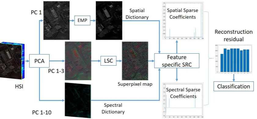
[image:4.595.88.509.478.673.2]Inspired by the aforementioned challenges and the success of SRC in HSI classification, we propose an improved SRC-based framework for the HSI classification. The framework consists of two components: superpixel generation, and kernel based SRC with proximity constraint using the online metric learning. Figure1shows the flowchart of the proposed framework, with the details discussed as follows.
Figure 1.The flowchart of the proposed SPFS-SRC framework.
2.2.1. Superpixel Generation
the LSC algorithm [36]. The LSC algorithm runs efficiently in linear complexity, which can optimize the segmentation cost function of normalized cut by applying the weighted k-means clustering strategy. The LSC algorithm proposes a novel relationship between the objective functions of the normalized cut and weighted k-means. Both objective functions can be equivalently optimised when the similarity between two points is equal to the weighted inner product between the two corresponding vectors [36]. During the superpixel generation process in our framework, the seeds are initialized with fixed spacing intervals in the false-colored image, and each seed is moved to its lowest neighbour. For each cluster, a weighted mean and a search center are calculated iteratively until the weighted means converge for all clusters. After grouping tiny superpixels, a superpixel map of HSI can be generated.
2.2.2. Superpixel-Based SRC
After creating the superpixel map, the original HSI can be divided into many spatial regions. Similar to the JSRC, pixels in each superpixel can be stacked into a matrixYi = [yi,1, ...yi,ni], where irepresents the index of the superpixel andni denotes the number of pixels it contains. Because we assume that pixels in one superpixel share the same spectral characteristics, all those pixels are considered jointly in our SRC framework.
With a 3-D cube of the HSI, rich spatial information is contained along with the spectral information. The EMPs are extracted to represent the spatial information. With the EMPs and the raw spectral data, fusion of the spectral-spatial features can be applied into the HSI classification. Although it is very straightforward to stack the spatial feature and spectral feature together, the derived high dimensional data may lead the overfitting. In [32], a simple weighted strategy is applied into the calculation of the reconstruction residual, where the weights of all extracted features are defined empirically. In [33], an adaptive weight strategy is designed, which sets a high penalty to the zero sparse coefficients based on the previous iteration. In the Multiple Feature Adaptive SRC (MFASR) [34] approach, the label of the test pixel is also determined by the sum of residuals from all extracted features. However, for the above methods, the significance of each extracted feature is not used, as most of them consider each feature equally. It is crucial to consider the difference among extracted features and preserve the regulariztion between the test and training samples.
To this end, we impose an learned distance on the joint sparse representation constraint. The SRC problem can be modified accordingly as:
ˆ
Ak=arg min A
K
∑
1
||Yk−Dk∗Ak||2+λ∗ k
∑
1
||BkKAk|| (6)
wherek=1, ...,Kis the index of the extracted features, andYK,DkandAkare the test pixel matrix, dictionary and sparse coefficients matrix in thekth feature. TheBkis the learned distance in thekth feature andJ
represents the element-wise multiplication.
With the learned distance between test samples and training samples, the training samples which are more closed to the test ones would be used for the reconstruction, which is corresponding to the fact that similar samples are more likely to be in the same class. Therefore, we introduce an online metric learning strategy to preserve the locality of data between the test sample and training samples. Generally, the predefined Euclidean distance is employed to measure the data similarity. In this paper, we have applied an Mahalanobis-based distance to find the matching between the test and training samples with multiple features, which guarantees to obtain more accurate sparse coefficients [38,39]. The distance function between two samplesx1andx2in thekth feature is defined as follows:
ˆ Bk(xk
1,x2k) =
q
ωkgk(xk1,xk2) (7)
whereωkis a nonnegative weight with thekth feature, and it is constrained by∑K1ωk=1;gk(xk1,xk2) =
(xk
Inspired by the LogDet Extract Gradient Online (LEGO) algorithm [38] and its application in visual tracking [39], our proposed method aims to learn the feature weightωand distance metricMK
iteratively. By acquiring the training sample pairs from the built dictionary for classification, we first defined two determination statementsφ1andφ2for the training sample pairs. If the two samples in
one training sample pair comes from the same class, we assume that the ground truth of this training sample pair is “similar”, the conditionφ1is described as:
φ1=
(
True, if gkp−1(x1k,xk2) = (xk1−xk2)TMkp−1(xk1−xk2)≥θ1
Flase, otherwise (8)
wherep=1, ...,Prepresents the number of iteration andPis equal to the number of training sample pairs;θ1is the threshold for determining the similarity of training sample pair.Mkp−1is the learned
metric from the last iteration andgkp−1is the related distance function. If theφ1holds true, the two
samples in this part does not match the ground truth, otherwise this pair matches the ground truth. Likewise, if the two samples in one training sample pair comes from different classes, we assume that the ground truth of this training sample pair is “dissimilar”, the statement is depicted as:
φ2=
(
True, if gkp−1(x1k,xk2) = (xk1−xk2)TMkp−1(xk1−xk2)≤θ2
Flase, otherwise (9)
If theφ2holds true, the two samples in this pair does not match the ground truth. Otherwise, the
determination is corresponding to the ground truth.
Although the training sample pairs can be acquired from the built dictionary before classification, we design an online based metric learning process to fully exploit the correlation between the training sample pairs. The training sample pairs of each feature are selected randomly to learn the Mahalanobis metricMk. For the feature weightωk, it is updated by using the Hedge algorithm [40]. With all selected
training sample pairs, the weight and metric for each feature are obtained as follows:
(1) Weight updating
The weight for each feature can be estimated using the Hedging algorithm as follows [40]:
ˆ
ωk,p=ωk,p−1βξ (10)
ωk,t=
ˆ
ωk,p
∑K
1ωk,p
(11)
whereβ ∈ (0, 1)is a penalty coefficient; if the training sample pair for thekth feature meets
the conditions in Equations (8) or (9), we haveξ=1, otherwise it is 0. if the determined result
of the training sample pair for thekth feature is against the ground truth, the feature weight is penalized.
(2) Metric Updating
According to the LEGO algorithm [38], if the training sample pair for thekth feature is punished based on the judgement, the Mahalanobis metricMkis updated by:
Mk,p=Mk,p−1−η(v−td)M
k,p−1(xk,p 1 −x
k,p
2 )(x
k,p
1 −x
k,p
2 )TMk,p−1
1+η(v−td)(x1k,p−xk2,p)Mk,p−1(x1k,p−x2k,p)
(12)
v = ηtd(x k,p
1 −x
k,p
2 )Mk,p−1(x
k,p
1 −x
k,p
2 )−1+
q
(ηtd(xk1,p−xk2,p)Mk,p−1(xk1,p−xk2,p)−1)2+4η((x1k,p−xk2,p)Mk,p−1(x1k,p−xk2,p))2
2η(xk1,p−xk2,p)Mk,p−1(x1k,p−xk2,p)
,
The proposed weight and metric updating algorithm is summarized in Algorithm 1. With the obtained metric and feature weights, the distanceBkcan be calculated. During the training process, the obtained Mahalanobis-based metric can be more discriminative to reflect the importance of each feature.
Algorithm 1Online metric learning.
1: Input: initialize feature weightωk0= K1; MetricMk0,k=1, ...,K;β;η;
2: Initialisation: GeneratePtraining sample pairs randomly: (xk1,p),(xk2,p), wherep =1, ...,Pand
k=1, ...K.
3: forp=1 toPdo
4: fork=1 toKdo
5: case1: % similar pairs
6: ifφ1holds truethen
7: ξ=1, update weightωk,pby (10) andMkpby (12);
8: else
9: ξ=0
10: end if
11: case2: % dissimilar pairs
12: ifφ2holds truethen
13: ξ=1, update weightωk,pusing Equation (10) andMkpusing Equation (12);
14: else
15: ξ=0
16: end if
17: end for
18: Update weight by (11);
19: end for
20: Output: Mk,k=1, ...,Kandω
k,k=1, ...K;
Since we have extracted the EMPs as the spatial features, the kernel based SRC is utilized to estimate the sparse coefficients for improving the non-linear separability of SRC:
ˆ
Akφ=arg min Aφ
K
∑
1
||Yφk−Dkφ∗Akφ||2+λ∗ k
∑
1
||BkKAkφ|| (13)
where the radial basis function (RBF) is used as the operated kernel function, andφrepresents the
kernel domain. With the estimated sparse coefficients in each feature, the label for all pixels of the superpixel can be assigned to the class with the minimum sum of residuals from multiple features:
ˆ
c=arg min c=1,...,C
K
∑
1
||Yφk−Dkφ,c∗Aˆkφ,c||2 (14)
Algorithm 2SPFS-SRC.
1: Input: raw HSI data
2: Feature extraction: Utilize PCA to extract principle components and then use the first component to generate EMPs as the spatial feature.
3: Superpixel generation: Apply the LSC algorithm to create superpixel map by using the first three components of HSI.
4: Metric learning: Learn the weight of each feature and update the distance between training samples and test samples.
5: Superpixel classification: Classify each superpixel based on SRC and learned metrics.
6: Output: Classification map;
3. Experimental Results
3.1. Datasets
To demonstrate the performance of our proposed framework, two publicly available remote sensing datasets have been used. The first one is the Pavia University (PaviaU) dataset, which is collected by the Reflective Optics System Imaging Spectrometer (ROSIS) sensor over the urban area surrounding the University of Pavia, Italy. With the ROSIS sensor, a HSI with the spatial resolution of 1.3 m/pixel and the spectral range between 0.43 to 0.86µm were captured. The PaviaU dataset has 103 spectral bands and its spatial size is 610×610. As part of the image has no information, a cropped image of 610×340 pixels is employed in the experiment. This dataset has 42776 labelled samples in 9 semantic categories, the number of samples in each class are quite unbalanced. The details of the PaviaU dataset and the generated superpixel map are shown in Figure2.
[image:8.595.91.505.422.662.2](a) (b) (c)
Figure 2.The superpixel generation process of the PaviaU dataset. (a) the ground truth, (b) the first three components of the HSI data, (c) the produced superpixel map.
dataset, for instance, there are only 20 labelled samples in the semantic class “oats”. Figure3shows the reference image of the Indian Pine dataset and the generated superpixel map.
[image:9.595.93.503.125.267.2](a) (b) (c)
Figure 3.The superpixel generation process of the Indian Pine dataset. (a) the ground truth, (b) the first three components of the HSI data, (c) the produced superpixel map.
3.2. Parameter Settings
In this paper, three common metrics have been used for quantitative performance evaluation, including the overall accuracy (OA), the average accuracy (AA) and the Kappa coefficient. OA reflects the percentage of correctly classified pixels, whilst AA denotes the mean of the class based classification accuracy. The Kappa coefficient represents the consistency of the classification result, which is estimated based on the confusion matrix. For these two datasets, the training data are selected randomly from all samples and the rest are used for testing. All experiments are completed with a 16 GB Intel i5-6500 CPU on the MATLAB 2017b.
In our online metric learning strategy, there are four predefined parameters, which include: two thresholdsθ1,θ2, the discounting parameterβand one regularization parameterη. To validate
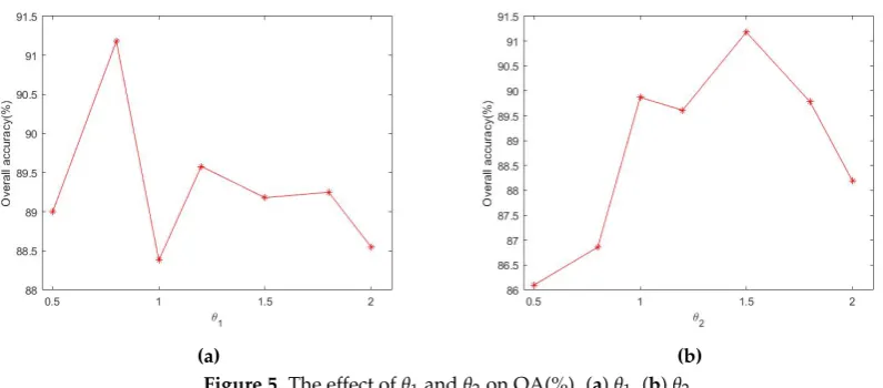
the effect of those four parameters on the OA, related experiments are carried out on both datasets. For the PaviaU dataset, 20 randomly selected training samples per class are used to train the classifier. In total we have 180 training sample pairs from 9 classes, include 90 “similar” pairs and 90 “dissimilar” training pairs, to guarantee the metric learning approach. The experimental results are shown in Figures4and5, and all experiments are repeated 10 times, where the OA is the average value on the 10 experiments.
[image:9.595.94.493.540.711.2](a) (b)
(a) (b) Figure 5.The effect ofθ1andθ2on OA(%). (a)θ1, (b)θ2.
As seen in Figure4, the discounting parameterβand the regularization parameterηhave limited
effect on the OA, from which we can assume that our approach is insensitive to these two parameters. In our experiments, the penalization parameter is chosen as 0.9, and ηis set to 0.2 as suggested
in [38,39]. For two thresholdsθ1andθ2, they were set to 0.8 and 1.5 according to Figure5, respectively.
For the Indian Pine dataset, same parameters are adopted while 16 “similar” sample pairs and 16 “dissimilar” sample pairs have randomly chosen from the training samples.
3.3. Comparison Experiments
To evaluate the performance of our framework under the situation of a small number of training samples, we have compared our framework with some state-of-the-art algorithms, including the support vector machine (SVM), the composite kernel support vector machine (CK-SVM) [15], the JSRC and the JKSRC [24,25], the MASR [27], the MFASR [34]. To better detect the effect of the our proposed online metric learning approach, a superpixel-based SRC model (SPSRC) without metric learning is also applied.
The parameter settings for the proposed approach and other compared methods are summarized as follows. The parameters of the proposed SPFS-SRC method, the SPSRC method, and the SVM-based algorithm, including kernel parameters and the reguralization parameters, are all determined via cross-validation. For JSRC and JKSRC, the default parameters suggested in [15] are adopted yet based on our own implementation of the algorithms. For other methods including CK-SVM, MASR and MFASR, experiments are tested on original codes with the default parameters. For CK-SVM and MFASR, the same spatial and spectral features are utilized for consistency. In addition, for all SRC-based methods, the sparsity level is set to 3 for efficiency.
Table 1.Number of training and testing samples in each class for the PaviaU dataset.
PaviaU Dataset
Class Sample Class Class
Label Name Train Test Label Name Train Test
1 Asphalt 20 6611 6 Bare Soil 20 5009 2 Meadows 20 18,629 7 Bitumen 20 1310 3 Gravel 20 2079 8 Self-blocking bricks 20 3662
4 Trees 20 3044 9 Shadows 20 927
[image:11.595.119.474.260.428.2]5 Painted metal sheets 20 1325 Total 180 42,596
Table 2.Number of training and testing samples in each class for the Indian Pine dataset.
Indian Pine Dataset
Class Sample Class Class
Label Name Train Test Label Name Train Test
1 Alfalfa 2 44 9 Oats 2 18 2 Corn-notill 14 1414 10 Soybeans-notill 10 962 3 Corn-min 9 821 11 Soybeans-min 25 2430 4 Corn 3 234 12 Soybeans-clean 7 586 5 Grass/pasture 5 478 13 Wheat 3 202 6 Grass/trees 8 722 14 Woods 13 1252 7 Grass/pasture-mowed 2 26 15 Bldg-gass-tree drives 4 382 8 Hay-windowed 5 473 16 Stone-steel towers 2 91
Total 114 10,135
Table 3.Classification results from different approaches for the PaviaU dataset with 20 training samples per class (Best result of each row is marked in bold type).
Methods SVM CK-SVM JSRC JKSRC MASR MFASR SPSRC SPFS-SRC
OA (%) 78.04±0.04 89.05±0.03 64.12±0.04 73.81±0.04 78.97±0.03 84.16±0.02 88.98±0.03 91.51±0.01 AA (%) 81.64±0.01 94.03±0.01 53.40±0.05 66.53±0.04 73.00±0.03 95.65±0.01 85.80±0.03 88.92±0.02 Kappa 0.68±0.04 0.86±0.04 0.61±0.04 0.75±0.02 0.82±0.01 0.86±0.02 0.91±0.01 0.92±0.01 Time (s) 6.12±0.01 11.12±0.03 61.99±0.01 57.80±0.01 331.87±12.57 266.05±10.87 5.77±0.02 12.1±0.01
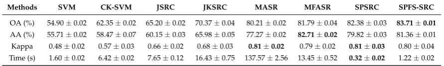
Table 4.Classification results from different approaches for the Indian Pine dataset with 1% training samples (Best result of each row is marked in bold type).
Methods SVM CK-SVM JSRC JKSRC MASR MFASR SPSRC SPFS-SRC
OA (%) 54.90±0.02 62.35±0.02 65.20±0.02 70.37±0.04 80.21±0.02 81.79±0.04 82.38±0.03 83.71±0.01
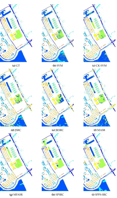
[image:11.595.78.516.472.526.2] [image:11.595.75.521.571.638.2](a)GT (b)SVM (c)CK-SVM
(d)JSRC (e)JKSRC (f)MASR
[image:12.595.106.494.74.727.2](g)MFASR (h)SPSRC (i)SPFS-SRC
(a)GT (b)SVM (c)CK-SVM
(d)JSRC (e)JKSRC (f)MASR
[image:13.595.88.495.82.509.2](g)MFASR (h)SPSRC (i)SPFS-SRC
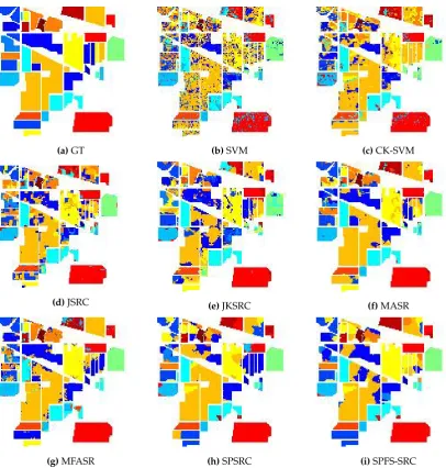
Figure 7.The classification map of the Indian Pine dataset. (a) the Ground Truth (GT), (b) SVM, (c) CK-SVM, (d) JSRC, (e) KSRC, (f) MASR, (g) MFASR, (h) SPSRC, (i) SPFS-SRC.
Table 5.The confusion matrix of the proposed SPFS-SRC from the PaviaU dataset corresponding to Table3.
Predicted
Gr
ound
T
ruth
Class 1 2 3 4 5 6 7 8 9
1 6278.8 0 2.3 78 0 0 0 152 7.1
2 0.7 16721.4 0 133.8 0 332.1 0 4.7 0 3 81.2 159.9 1945.5 13.9 0 0 0 183.6 52.6 4 13.8 262.7 5.4 2772.1 0 0 0 52.9 0
5 0 0 0 0 1282.6 0 0 0 63.9
6 0.3 1381.5 0 6.6 0 4676.9 15.5 0 0
7 94.6 0 0 2 0 0 1281.9 0.8 49.1
8 141.6 13.5 110.8 34.6 0 0 0 3268 9.1
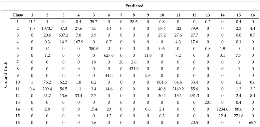
[image:13.595.122.475.583.738.2]Table 6.The confusion matrix of the proposed SPFS-SRC from the Indian Pine dataset corresponding to Table4.
Predicted
Gr
ound
T
ruth
Class 1 2 3 4 5 6 7 8 9 10 11 12 13 14 15 16
1 41.1 1 0 0.4 39.7 0 0 38.5 0 0.8 0 0 0.2 0 0.4 0
2 1.5 1070.7 37.3 21.6 1.5 1.4 0 0 0 58.4 122 79.9 0 0 2.3 4.4
3 0 20.6 637.2 7.8 3.9 0 0 0 0 27.2 27.6 27.7 0 0 0.8 8.7
4 0 0.3 14.2 167.9 0 0.7 0 0 0 0 4.3 17.6 0 0 0.1 0
5 0 0.1 0 0 380.6 0 0 0 0 0.6 0 0 0.8 1.9 0 0
6 0 1.2 0 0 0 627.6 0 0 11.8 0 7.2 0 0 3.1 7.7 0
7 0 0 0 0 18 0 26 2.6 0 0 0 0 0 0 0 0
8 0 0 0 0 0 0 0 431.9 0 0 0 0 0 0 0 0
9 0 0 0 0 0 44.5 0 0 5.6 0 0 0 0 0 0 0
10 1 76.2 62.2 1.8 6.2 0 0 0 0 801.6 84.6 33.4 0 0 6.2 0.6
11 0.4 209.4 56.5 1.1 3.4 14.6 0 0 0 40.8 2169.2 55.6 0 0 1.3 3.2
12 0 31.7 13.6 33.4 7.7 0 0 0 0 30.2 15.1 351.3 0 0 2.4 8.4
13 0 0 0 0 0 0 0 0 0 0 0 0 201 0 0.4 0
14 0 2.8 0 0 15.4 29 0 0 0.6 2.1 0 0 0 1234.6 88.6 0
15 0 0 0 0 0 4.2 0 0 0 0.3 0 0 0 12.4 271.8 0
16 0 0 0 0 1.6 0 0 0 0 0 0 20.5 0 0 0 65.7
As seen in Tables3and4, our proposed framework achieves the best performance in the PaviaU dataset with only 20 training samples per class. Many algorithms cannot gain satisfactory classification result even with the aid of the spatial information. It can be noticed that our proposed method performs better than our baseline approach, where the OA is improved about 2.5% after the utilization of the online metric learning strategy. This has clearly demonstrated the efficacy of this strategy and the Mahalanobis-based distance. In the Indian Pine dataset, our approach also achieves the hightest OA among all compared algorithms. With the aid of the weight from the online metric learning strategy, the OA is also improved from the baseline approach.
4. Discussion and Conclusion
During the last several years, various approaches have been proposed to improve the performance of HSI classification. In this paper, we propose a superpixel-based feature specific SRC framework to fully exploit the spectral-spatial features of the HSI. A superpixel map is generated to acquire better spatial information and save computational cost. After the superpixel generation, a SRC-based classifier is designed to assign each superpixel into certain category. With our proposed SRC-based classifier, it can be noticed that our approach achieves a better performance than other methods in both datasets.
In this paper, we have also designed an online Mahalanobis-based metric learning strategy to acquire better matching between the training and test samples. With this mechanism, we have achieved the best performance in both datasets, and we also improve the OA in the PaviaU dataset from the baseline method’s 88.98% to 91.51%, and in Indian Pine dataset from 82.38% to 83.71%. From the experimental reuslts, the learned metric can improve the discriminative ability of the SRC without high computational burden. For the learned metric, four determined parameters are discussed. For the discounting parameterβand regularization parameterη, corresponding results show that these two
parameters are robust to the OA. As for the two thresholdsθ1andθ2that determined the defined
On the other hand, there may be also small regions of ’bare soil’ in labelled ’meadows’ regions. This explains the high error rate from class 6 to class 2, yet the low error rate from class 2 to class 6.
The future work can be summarized as follows: firstly, we will work on a more reliable superpixel generation approach, aiming to produce superpixels for classification and maintain the superpixel boundaries to adhere well to the natural boundaries. Especially for small images like the Indian Pine dataset, a more accurate superpixel map is desirable. Secondly, we will dedicate to design a more robust online metric learning strategy, which can reduce the number of parameters and provide even better matching between training samples and test sample. Thirdly, for our framework, more features will be explored in the future, even with an automatic feature selection method such as band selection [41–43].
Author Contributions:Conceptualization, J.R. and H.Z.; methodology, H.S. Y.Y. and J.Z.; software, H.S.; validation and analysis, all; writing–original draft preparation, H.S.; writing–review and editing, J.R.; supervision, J.R.; project administration and funding acquisition, J.R.
Funding:This research was funded by Engineering the Future Scholarship, Faculty of Engineering, University of Strathclyde, Guangdong Key Laboratory of Intellectual Property Big Data (No.2018030322016), the National Natural Science Foundation of China (61672008), Guangdong Provincial Application-oriented Technical Research and Development Special Fund Project, and Scientific and Technological Projects of Guangdong Province (2017A050501039).
Acknowledgments: The Authors would like to thank D. Landgrebe and P. Gamba for providing two remote sensing datasets. We would also like to thank L. Fang and J. Li for providing the online codes of MASR, MFASR and CK-SVM.
Conflicts of Interest:The authors declare no conflict of interest.
References
1. Zabalza, J.; Ren, J.; Zheng, J.; Han, J.; Zhao, H.; Li, S.; Marshall, S. Novel two-dimensional singular spectrum analysis for effective feature extraction and data classification in hyperspectral imaging.IEEE Trans. Geosci. Remote Sens.2015,8, 4418–4433. [CrossRef]
2. Zabalza, J.; Qing, C.; Yuen, P.; Sun, G.; Zhao, H.; Ren, J. Fast implementation of two-dimensional singular spectrum analysis for effective data classification in hyperspectral imaging.J. Franklin.2018,4, 1733–1751. [CrossRef]
3. Wang, C.; Ren, J.; Wang, H.; Zhang, Y.; Wen, J. Spectral-spatial classification of hyperspectral data using spectral-domain local binary patterns.Multimed. Tools Appl.2018,22, 29889–29903. [CrossRef]
4. Zhao, C.; Li, X.; Ren, J.; Marshall, S. Improved sparse representation using adaptive spatial support for effective target detection in hyperspectral imagery.Int. J. Remote Sens.2013,24, 8669–8684. [CrossRef] 5. Ma, D.; Yuan, Y.; Wang, Q. Hyperspectral Anomaly Detection via Discriminative Feature Learning with
Multiple-Dictionary Sparse Representation.Remote Sens.2018,5, 745. [CrossRef]
6. Sun, G.; Zhang, A.; Ren, J.; Ma, J.; Wang, P.; Zhang, Y.; Jia, X. Gravitation-based edge detection in hyperspectral images.Remote Sens.2017,6, 592. [CrossRef]
7. Chen, M.; Wang, Q.; Li, X. Discriminant Analysis with Graph Learning for Hyperspectral Image Classification. Remote Sens.2018,6, 836. [CrossRef]
8. Zabalza, J.; Ren, J.; Wang, Z.; Marshall, S.; Wang, J. Singular spectrum analysis for effective feature extraction in hyperspectral Imaging.IEEE Geosci. Remote Sens. Lett.2014,11, 1886–1890. [CrossRef]
9. Cao, F.; Yang, Z.; Ren, J.; Ling, W.; Zhao, H.; Sun, M.; Benediktsson, J.A. Sparse representation-based augmented multinomial logistic extreme learning machine with weighted composite features for spectral-spatial classification of hyperspectral images.IEEE Trans. Geosci. Remote Sens.2018,99, 1–17. [CrossRef]
10. Cao, F.; Yang, Z.; Ren, J.; Ling, W.; Zhao, H.; Sun, M. Extreme sparse multinomial logistic regression: A fast and robust framework for hyperspectral image classification.Remote Sens.2017,9, 1255. [CrossRef] 11. Qiao, T.; Yang, Z.; Ren, J.; Yuen, P.; Zhao, H.; Sun, G.; Marshall, S.; Benedktsson, JA. Joint bilateral filtering
12. Qiao, T.; Ren, J.; Wang, Z.; Zabalza, J.; Sun, M.; Zhao, H.; Li, S.; Benediktsson, J.A.; Dai, Q.; Marshall, S. Effective denoising and classification of hyperspectral images using curvelet transform and singular spectrum analysis.IEEE Trans. Geosci. Remote Sens.2017,1, 119–133. [CrossRef]
13. Ham, J.; Chen, Y.; Crawford, M.; Ghosh, J. Investigation of the random forest framework for classification of hyperspectral data.IEEE Trans. Geosci. Remote Sens.2005,3, 492–501. [CrossRef]
14. Chen, Y.; Jiang, H.; Li, C.; Jia, X.; Ghamisi, P. Deep feature extraction and classification of hyperspectral images based on convolutional neural networks. IEEE Trans. Geosci. Remote Sens. 2016,10, 6232–6251. [CrossRef]
15. Li, J.; Marpu, P. P.; Plaza, A.; Bioucas-Dias, J.; Benediktsson, J.A. Generalized composite kernel framework for hyperspectral image classification.IEEE Trans. Geosci. Remote Sens.2013,9, 4816–4829. [CrossRef] 16. Xia, J.; Ghamisi, P.; Yokoya, N.; Iwasaki, A. Random forest ensembles and extended multiextinction profiles
for hyperspectral image classification.IEEE Trans. Geosci. Remote Sens.2018,1, 202–216. [CrossRef] 17. Zhong, Y.; Lin, Y.; Zhang, L. A support vector conditional random classifier with a Mahalanobis distance
boundary constraint for high spatial resolution remote sensing imagery.IEEE J. Sel. Topics Appl. Earth Observ. Remote Sens.2014,4, 1314–1330. [CrossRef]
18. Qing, C.; Ruan, J.; Xu, X.; Ren, J.; Zabalza, J. Spatial-spectral classification of hyperspectral images: A deep learning framework with Markov Random fields based modelling. IET Image Process. 2019,13, 235–245. [CrossRef]
19. Prasad, S.; Mann Bruce, L. Limitations of principle component analysis for hyperspectral target recognition. IEEE Geosci. Remote Sens. Lett.2008,4, 625-629. [CrossRef]
20. Zabalza, J.; Ren, J.; Yang, M.; Zhang, Y.; Wang, J.; Marshall, S.; Han, J. Novel Folded-PCA for improved feature extraction and data reduction with hyperspectral imaging and SAR in remote sensing. ISPRS J. Photogramm. Remote Sens.2014,93, 112–122. [CrossRef]
21. Benediktsson, J. A.; Palmason, J. A.; Sveinsson, J.R. Classification of hyperspectral data from urban areas based on extended morphological profiles.IEEE Trans. Geosci. Remote Sens.2005,3, 480–491. [CrossRef] 22. Ghamisi, P.; Souza, R.; Benediktsson, J.A.; Zhu, X.X.; Rittner, L.; Lotufo, R.A. Extinction profiles for the
classification of remote sensing data.IEEE Trans. Geosci. Remote Sens.2016,10, 5631–5645. [CrossRef] 23. Wright, J.; Yang, A.Y.; Ganesh, A.; Sastry, S.S.; Ma, Y. Robust face recognition via sparse representation.
IEEE Trans. Pattern. Anal.2009,2, 210–227. [CrossRef] [PubMed]
24. Chen, Y.; Nasrabadi, M.M.; Tran, T.D. Hyperspectral image classification using dictionary-based sparse representation.IEEE Trans. Geosci. Remote Sens.2011,10, 3973–3985. [CrossRef]
25. Chen, Y.; Nasrabadi, M.M.; Tran, T.D. Hyperspectral image classification via kernel sparse representation. IEEE Trans. Geosci. Remote Sens.2013,1, 217–231. [CrossRef]
26. Zhang, H.; Li, J.; Huang, Y.; Zhang, L. A nonlocal weighted joint sparse representation classification method for hyperspectral imagery.IEEE J. Sel. Top. Appl. Earth Observ. Remote Sens.2014,6, 2056–2065. [CrossRef] 27. Fang, L.; Li, S.; Kang, X.; Benediktsson, J.A. Spectral-spatial hyperspectral image classification via multiscale
adaptive sparse representation.IEEE Trans. Geosci. Remote Sens.2014,12, 7738–7749. [CrossRef]
28. Zhan, T.; Sun, L.; Xu, Y.; Yang, G.; Zhang, Y.; Wu, Z. Hyperspectral image classification via superpixel kernel learning-based low rank representation.Remote Sens.2018,10, 1639. [CrossRef]
29. Fu, W.; Li, S.; Fang, L.; Kang, X.; Benediktsson, J.A. Hyperspectral image classification via shape-adaptive joint sparse representation.IEEE J. Sel. Top. Appl. Earth Observ. Remote Sens.2016,2, 556–567. [CrossRef] 30. Fang, L.; Li, S.; Duan, W.; Ren, J.; Benediktsson, J.A. Classification of hyperspectral images by exploiting
spectral-spatial information of superpixel via multiple kernels.IEEE Trans. Geosci. Remote Sens. 2015,12, 6663–6674. [CrossRef]
31. Fang, L.; Li, S.; Kang, X.; Benediktsson, J.A. Spectral-spatial classification of hyperspectral images with a superpixel-based discriminative sparse model. IEEE Trans. Geosci. Remote Sens. 2015, 8, 4186–4201. [CrossRef]
32. Li, J.; Zhang, H.; Zhang, L.; Huang, X.; Zhang, L. Joint collaborative representation with multitask learning for hyperspectral image classification.IEEE Trans. Geosci. Remote Sens.2015,9, 5923–5936.
33. Zhang, Y.; Prasad, S. Multisource geospatial data fusion via local joint sparse representation.IEEE Trans. Geosci. Remote Sens.2016,6, 3265–3276. [CrossRef]
35. Gan, L.; Xia, J.; Du, P.; Chanussot, J. Multiple feature kernel sparse representation classifier for hyperspectral imagery.IEEE Trans. Geosci. Remote Sens.2018,9, 5343–5356. [CrossRef]
36. Li, Z.; Chen, J. Superpixel segmentation using linear spectral clustering. In Proceedings of the IEEE Conference on Computer Vision and Pattern Recognition (CVPR 2015), Boston, MA, USA, 8–10 June 2015; pp. 1356–1363.
37. Pati, Y.C.; Rezaiifar, R.; Krishnaprasad, P.S. Orthogonal matching pursuit: Recursive function approximation with applications to wavelet decomposition. In Proceedings of the 27th Asilomar Conference on Signals, Systems and Computer, Pacific Grove, CA, USA, 1–3 November 1993; pp. 40–44.
38. Jain, P.; Kulis, B.; Dhillon, I.S. Grauman, K. Online metric learning and fast similarity search. In Proceedings of the Advances in Neural Information Processing Systems 21 (NIPS 2008), Vancouver, BC, Canada, 8–10 December 2008; pp. 761–768.
39. Lan, X.; Zhang, S.; Yuen, P.C.; Chellappa, R. Learning common and feature-specific patterns: A novel multiple-sparse-representation-based tracker. IEEE Trans. Image. Process. 2018,4, 2022–2037. [CrossRef] [PubMed]
40. Freund, Y.; Schapire, R.E. A decision-theoretic generalization of on-line learning and an application to boosting.J. Comput. Syst. Sci.1997,1, 119–137. [CrossRef]
41. Tschannerl, J.; Ren, J.; Yuen, P.; Sun, G.; Zhao, H.; Yang, Z.; Wang, Z.; Marshall, S. MIMR-DGSA: Unsupervised hyperspectral band selection based on information theory and a modified discrete gravitational search algorithm.Inform Fusion.2019, in press. [CrossRef]
42. Li, Q.; Wang, Q.; Li, X. An efficient clustering method for hyperspectral optimal band selection via shared nearest neighbor.Remote Sens.2019,11, 350. [CrossRef]
43. Chen, W.; Yang, Z.; Cao, F.; Yan, Y.; Wang, M.; Qing, C.; Cheng, Y. Dimensionality reduction based on determinantal point process and singular spectrum analysis for hyperspectral images.IET Image Process. 2019,13, 299–306. [CrossRef]
c