City, University of London Institutional Repository
Citation
:
Vlahakis, E. E. ORCID: 0002-7039-5314 and Halikias, G. ORCID:
0000-0003-1260-1383 (2019). Temperature and concentration control of exothermic chemical
processes in continuous stirred tank reactors. Transactions of the Institute of Measurement
and Control, 41, pp. 4274-4284. doi: 10.1177/0142331219855591
This is the accepted version of the paper.
This version of the publication may differ from the final published
version.
Permanent repository link:
http://openaccess.city.ac.uk/id/eprint/22990/
Link to published version
:
http://dx.doi.org/10.1177/0142331219855591
Copyright and reuse:
City Research Online aims to make research
outputs of City, University of London available to a wider audience.
Copyright and Moral Rights remain with the author(s) and/or copyright
holders. URLs from City Research Online may be freely distributed and
linked to.
Temperature and concentration control
of exothermic chemical processes in
continuous stirred tank reactors
Journal Title XX(X):1–10
c
The Author(s) 2018 Reprints and permission:
sagepub.co.uk/journalsPermissions.nav DOI: 10.1177/ToBeAssigned www.sagepub.com/
SAGE
Eleftherios Vlahakis
1and George Halikias
1Abstract
Exothermic chemical reaction taking place in continuous stirred tank reactor is considered. Heat release from the chemical reaction, non-linear dynamic behavior of the process and uncertainty in parameters are the main factors motivating the use of robust control design. Viewing temperature and molar concentration as variables both accessible in real time, PI and optimal state-feedback controllers driven by temperature and concentration error signals are proposed to regulate the system over reactor’s steady-state working points by counteracting undesired disturbances. Since access to concentration value has proved beneficial for the reactor’s performance, estimation techniques are examined to compensate for the problematic nature of the concentration’s measurement. A linear reduced-order observer is first proposed to estimate the concentration value using temperature measurements. In addition, assuming concentration measurement is available with a relatively short delay via sample analysis, a linear and non-linear discrete-time predictor is constructed to estimate the concentration’s real-time value. A linear combination of the two estimation schemes (observer, predictor) is proposed resulting in a combined estimator, in which the emphasis between the two individual schemes can be controlled via a scalar parameter. The work presented in this paper was supported by the GLOW project - New weather-stable low gloss powder coatings based on bifunctional acrylic solid resins and nanoadditives - as part of the development of novel and efficient processing technologies regarding the production of new families of powder coatings, responding to industrial requirements for quality improvement at lower cost and shorter development cycles.
Keywords
exothermic chemical reaction, continuous stirred tank reactor, PI control, state feedback, linear quadratic regulator (LQR), state estimation, reduced-order observer, linear/non-linear predictor, partial-state delay.
Introduction
Continuous stirred tank reactors (CSTR) (Ingham et al.,
2007; Shakeri et al., 2017) are examined as one of the
common devices where exothermic chemical reactions are taking place. The continuous operation of such reactors can provide high rates of production with possibly more constant product quality. Reactant preparation and product treatment also need to run continuously. The fact that the reactant is being fed continuously into the tank requires careful flow management. Also, more attention should be paid to the control design since the complexity of the system has been augmented by the feeder flow rate.
Due to exothermic reaction and the corresponding heat release of such processes, the control design turns out to be challenging, taking also into consideration the non-linearities of the system. Yet, model parameter uncertainty is another issue which has to be tackled and as a result robust control methods may be required. Conventional PID (proportional-integral-derivative) output feedback controllers have been traditionally applied to CSTR for temperature regulation due to their simplicity in terms of design and their robust performance to model uncertainties. Recent work on PID control for CSTR is presented in Banu and Uma (2008) and Baruah and Dewan (2017). Analytic studies on input-output linearizing control applied to continuous stirred tank reactors have been extensively carried out in
Jouili et al. (2008), Barkhordari Yazdi and Jahed-Motlagh
(2009) and Tofighi et al. (2017). Optimal linear control techniques have also been developed to guarantee stability of continuous stirred tank reactors based on linearization. A rigorous robust design methodology with H2 and H∞ performance for linear and nonlinear CSTR models has been presented in Guay et al. (2005), Komari Alaei and
Yazdizadeh (2014) andVasiˇckaninov´a et al. (2015). Model
predictive control (Mayne, 2014; Oravec and Bakoˇsov´a, 2015) has also received considerable attention by the process control research community. Other approaches include design methods based on multiple models (Kvasnica et al.,
2010; Krishnan et al., 2017) and techniques based on a
combination of neural networks and MPC or adaptive control
(Vasiˇckaninov´a and Bakoˇsov´a, 2009; Li, 2013). Rigorous
robust methods for CSTR’s based on Lyapunov stability concepts have been proposed inAntonelli and Astolfi,2003. Note that almost all existing methods proposed in the literature need the on-line measurement of the
1Research Centre for Systems and Control - City, University of London,
UK
Corresponding author:
Eleftherios Vlahakis, City, University of London, Northampton Square, London EC1V 0HB, United Kingdom.
Email: [email protected]
full state of the system, represented by the reactor’s temperature and the reactant’s molar concentration. In industrial practice the reactor’s temperature is quite easily accessible while the reactant’s molar concentration monitoring normally requires off-line analysis of samples which may involve considerable delays. Since real-time access to the concentration measurement might not be possible due to current technology cost, the designer has to consider estimation and prediction techniques. A classification of recent observers and a review on state and parameter estimation with application to chemical processes can be found in Mohd Ali et al. (2015) and Kravaris
et al. (2013), respectively. Nonlinear observer algorithms
for chemical processes have been presented in Botero
and ´Alvarez (2011) and Zhao et al. (2019). A recent
work on observer design for a class of nonlinear systems including unknown, bounded and time-varying delays has been presented in Naifar et al. (2016). In this work, exponential stability conditions are established with the use of Lyapunov-Krasovskii functionals.
From a process control implementation perspective, real-time monitoring of chemical reactions is very important. Typical measuring methods that require excessive time and intensive sample preparation might be ineffective or inappropriate for industrial process control. Recently, spectroscopic techniques (Hofmann,2010) have proved quite promising in terms of their precision and fast response. In particular, near-infrared (NIR) (Kim et al.,2000) analyzers provide rapid results while sample preparation can be eliminated by using suitable probes placed inside the reactor. The NIR spectroscopy may be characterized as off-line, at-line, on-line and in-line process (Bakeev,2005) with respect to the analysis strategy which is implemented. Off-line and at-line analysis require manual sampling and removal from the reactor with the analyzer being near the production line in the at-line case. Automated sampling and transport through a sample line to the analyzer is employed in the on-line method, while suitable probes connected to the analyzer are located inside the reactor in the in-line technique. The off-line is obviously a slow method and can provide results from several minutes to an hour. On the contrary, the in-line technique (Santos et al.,2005) may yield results very fast but can prove quite expensive due to equipment specifications.
Several methods proposed in the literature for solving the CSTR regulation problem do not take into consideration the problematic nature of the reactant’s concentration monitoring and assume that the entire state-vector is available for control in real-time without incorporating any delay resulting from sampling process. In contrast, various alternative methods rely on output feedback control without including molar concentration among the measured variables. Although these typically result in simple control schemes which are easy to implement they do not take into account important information about the process. In this paper we focus on CSTR systems which are equipped with a reactant’s concentration sensing system which provides measurements as a result of sample analysis. Therefore, the main motivation of our work is to present estimation techniques for such CSTR systems and compensate for possible limitations of the sensing system of the reactor which are mainly due to delayed measurements
of the reactant’s concentration variable (off-line testing, calibration). A combination of reduced-order observer and future predictor is proposed to estimate the real-time molar concentration value. Based on the separation principle we incorporate these estimation techniques into typical control schemes (PI and optimal control) and solve the reactor’s regulation problem.
Simulation results based on the nonlinear model of the continuous stirred tank reactor show that the system can be effectively controlled using simple PI and LQR controllers. Our analysis includes the dynamic behavior of the nonlinear system subject to disturbances and parametric uncertainty. The main contribution of our work is to propose a novel observer-based control scheme relying on two separate estimates of the molar concentration variable. The first is obtained from a reduced-order observer driven by the real-time temperature measurement while the second is a prediction constructed from delayed molar concentration measurement. Thus, the proposed scheme is parametric in nature and can be tuned depending on the relative accuracy of the model, the delay duration and the accuracy of the sensors. We believe that the method can be further developed theoretically in the context of MPC control for models with uncertain parameters and process/measurement noise, although this is beyond the scope of the present work.
Next, we discuss factors that may restrict the applicability of the proposed method in real applications. Since our approach is model-based, ignored dynamics arising due to impurities in the reactant’s composition as well as side-reactions taking place in the reactor may give rise to additional equilibrium points and result in deterioration of the controller performance. In addition, it is natural to expect that in the presence of very long delays the method will ultimately break down. In particular, our simulations studies suggest that in the absence of an observer the PI control scheme can tolerate a maximum delay of approximately five minutes in the concentration variable. However, the situation is significantly improved when an estimator is employed to compensate for the delayed measurements. Another potential limitation is that the nonlinear model does not have a unique equilibrium point and therefore regulation can be guaranteed only for disturbances of a sufficiently small magnitude. This has been explicitly taken into account during the design process and all control schemes are validated via nonlinear simulations. Control design limitations due to uncertainty in the values of k0 and∆H are also presented, see Table 3. Another source of uncertainty is introduced by scaling-up the control scheme from experimental to industrial level. All the above limitations constrain the implementation of the proposed method and should be examined carefully when real applications are considered.
The text is organized in five sections. The second section describes briefly the mathematical model of first-order irreversible chemical reaction taking place in a continuous stirred-tank reactor. The model is based on Vojtesek and
Dostal(2011) andGao et al.(2002) and illustrates clearly the
Vlahakis and Halikias 3
along with a discussion of the main results and suggestions for future work.
Reactor modelling
In this work a simple first-order chemical reaction is considered, described by the chemical equation of the form
A→products+energy (1)
where the term ”energy” accounts for heat release due to exothermic reaction.
The reaction is conducted in a continuous stirred tank reactor where the reactantAis prepared to enter the tank at an initial concentrationcA0and temperatureT0. The reactant
inside the tank is kept at specific conditions in terms of its molar concentrationcA and temperatureT according to
the working conditions or set-points of the reactor. These conditions are referred to as equilibrium points. Perfect mixing conditions inside the reactor are assumed. In this respect, it is assumed that the output composition is identical to the composition of the material inside the reactor and the mass and energy balance equations can be simplified. These equations are standard and can be found in (Ingham et al.,
2007).
Reactor’s Model and Stability Issues
Consider a simple first-order irreversible exothermic reaction
A→Bcarried out in a continuous stirred-tank reactor where the reaction rate isrA=k1CAand the cooling mechanism is assumed to be a coil heat exchanger. The same reactor’s model used inVojtesek and Dostal (2011) and Gao et al. (2002) has been chosen to illustrate clearly the main points of our work while avoiding unnecessary complications. We assume that reactant and coolant are perfectly mixed and also the volume of the reactor’s tank is constant.
The non-linear differential equations shown below represents the dynamic behavior of the main variables of the reactor’s system.
dT
dt =α1(T0−T) +α2k1cA
+a3qc(1−e
α4 qc)(Tc
0−T) (2)
dcA
dt =α1(cA0−cA)−k1cA (3)
where
α1=
q
V α2=
−∆H ρcp
α3=
ρccpc ρcpV
α4=
−hα ρccpc
(4)
The main nonlinearity of the model is due to reaction rate parameterk1, which is nonlinear function of the reactor’s temperatureT and it is computed from the Arrhenius law,
k1=k0e −E
RT. The fixed parameters of the system are shown in Table1.
Steady-state analysis
[image:4.595.52.291.541.656.2]The controlled variables in the mathematical model are the reactant’s feeding flow rateq (l·min−1) and the coolant’s flow rate qc (l·min−1). Therefore the control strategy
Table 1. Fixed parameters of the reactor (Vojtesek and Dostal,
2011).
Quantity Symbol, value and units
Reactor’s volume V = 100l
Reaction rate constant k0= 7.2·1010min−1
Activation energy toR E/R= 1·104K Reactant’s feed temperature T0 = 350K
Inlet coolant temperature Tc0 = 350K
Reaction heat ∆H=−2·105cal·mol−1
Specific heat of the reactant cp= 1cal·g−1·K−1
Specific heat of the coolant cpc= 1cal·g
−1·
K−1 Density of the reactant ρ= 1·103g·l−1 Density of the coolant ρc= 1·103g·l−1
Feed concentration CA0= 1mol·l
−1
Heat transfer coefficient hα= 7·105cal·min−1·K−1
depends on the decision we make on q and qc in order
to achieve the desired performance of the reactor. The steady-state analysis shows the behavior of the system in steady-state where the reaction process is expected to be constant and the transient phenomena have decayed considerably. As the system might have several steady-state working points, the optimal working conditions should be chosen with respect to maximal effectiveness as well as concentration yield. However, if at the optimal working point the temperature is too high, possible side reactions may take place or equipment issues may arise.
At steady state, the temperature and the concentration in the reactor are constant. Hence dTdt =dCA
dt = 0. Solving for T andcAwe get
csA= cA0
1 +k1V /q
(5)
Ts= α1T0+α2k1c
s
A+α3qc(1−e
α4
qc)
α1+α3qc(1−e
α4
qc)
(6)
which define the steady-state model.
Setting working points for the control variables q and
qc we can find the steady-state (equilibrium) values of
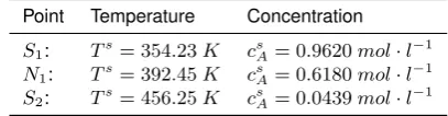
Ts and csA. If these do not satisfy reactor’s performance, new control values are considered until Ts and csA are acceptable. Therefore, the decision upon the choice of the steady-state of the state variables depends on the reactor’s performance as well as the actuators’ capacity. In this case study three steady-state points are obtained by solving the above algebraic equations for q= 100 l·min−1 andq
c=
80l·min−1. The state variables at these points are given in Table2.
Table 2. Steady States.
Point Temperature Concentration
S1: Ts= 354.23K csA= 0.9620mol·l−1
N1: Ts= 392.45K csA= 0.6180mol·l
−1
S2: Ts= 456.25K csA= 0.0439mol·l
−1
Stability of steady-state points
By considering the effect of small temperature variations, about the three steady-state conditions, it can be shown
(Ingham et al., 2007, p. 111) that the points S1 and S2
[image:4.595.320.524.656.709.2]represent stable operating conditions, whereas the middle intersection pointN1 is unstable. On start up, the reaction conditions will proceed to eitherS1orS2, depending on the initial conditions of the reactor. Since pointS1 represents a low temperature equilibrium, and therefore a low conversion operating state, it may be desirable that the initial transient should eventually lead to S2, rather than to S1. However if the temperature corresponding to point S2 is too high, this may lead to further decomposition reactions which are undesirable in which case pointS1may be preferable.
Linearization about steady-state points
Local system stability can be analyzed in terms of linearized differential equations. New perturbation variables for the temperature δT and the concentration δcA are defined in
terms of small deviations in the actual reactor conditions away from the steady-stateTsandcs
A:
δT =T−TsandδcA=cA−csA (7)
The linearization of the non-linear eq. (2) and (3) based on the use of Taylor’s expansion theorem leads to linear differential equation with constant coefficients of the form
˙
δT
˙
δcA
=
A11 A12
A21 A22
δT δcA
+
B11 B12
B21 B22
δq δqc
(8)
where δq=q−qs and δqc =qc−qs
c account for the
variations of the control variablesqandqcfrom the steady-state values (qs= 100mol·l−1,qs
c = 80mol·l−1).
A linear model is derived about the S2 (456.25,0.0439) steady-state point and the correspondingAandB matrices are given as follows
A=
7.397 4361
−0.046 −22.8
,B=
−1.062 −1.061 0.0096 0
(9)
Matrix A defines the dynamic behavior of the linearized system. The eigenvalues (−2.459,−12.948) of A are negative and the stable nature of S2 is verified. The linearization about an unstable equilibrium point is of theoretical interest only, since in practice, due to strong non-linearities and large uncertainties in model parameters, chemical reactors usually operate over stable equilibria points.
Problem Statement and Control Design
In this section, it is assumed that the operating point of the reaction has been selected. The problem which arises is the type of control that needs to be designed to counteract any deviation from the equilibrium conditions and avoid the possibility of thermal runaway. These may be due to external disturbances or discrepancies in the initial conditions of the reactant. Further, uncertainties in the model parameters, sensor noise or delays in the measurement channels could also affect the steady-state conditions of the reactor. As a result robust regulation is needed with the ability to reject disturbances despite the presence of uncertainty in the model. If state feedback control is employed the reactor’s state variables should be measured at real time. Temperature measurements can be easily obtained in real time but could
be noisy due to sensors’ imperfection. In contrast, the measurement of molar concentrationcAin real time is much
more problematic. In all cases, some delay between the sample analysis time and the measurement acquisition time is almost always present.
PI Control
At this point, we assume that both temperature and concentration signals are available and can be fed back to the inputs of the plant. The PI control structure is given as
u=Kpe+Ki
Z t
0
edτ (10)
whereeis the error signal (reference signal minus measured signal). Integral action results in zero steady-state error and fast disturbance rejection can be achieved by the appropriate tuning of Kp and Ki gains. In the following diagrams, PI
temperature control is applied to both coolant and feeder flow rate with the aim to reject pulse disturbances added to the input channels. The tuning of the gains has been implemented using standard techniques guided by simulation results.
0 5 10 15 20
Time [min]
445 450 455 460 465
Temperature [K]
Temperature PI control in both inputs
[image:5.595.312.529.347.485.2]pulse: duration 4 min with magnitude +5 pulse: duration 4 min with magnitude +50
Figure 1. Disturbance rejection using PI temperature control -Reactor’s temperature.
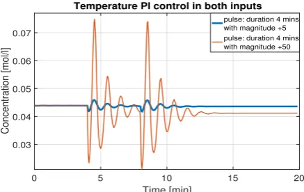
0 5 10 15 20
Time [min]
0.03 0.04 0.05 0.06 0.07
Concentration [mol/l]
Temperature PI control in both inputs
pulse: duration 4 mins with magnitude +5 pulse: duration 4 mins with magnitude +50
Figure 2. Disturbance rejection using PI temperature control -Reactor’s concentration.
[image:5.595.311.530.543.681.2]Vlahakis and Halikias 5
magnitude of the disturbance signal increases. This suggests that additional feedback control using the concentration measurement would be useful. The results of the combined scheme are shown in Fig. 3 and 4. Now both regulated variables vary considerably less after a pulse disturbance is applied to the feeder input. The response of the two reactor’s inputs for a time interval of 20 minutes after a larger disturbance pulse is applied is shown in Fig.5and6(for both control schemes).
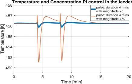
0 5 10 15 20
Time [min]
452 453 454 455 456 457 458
Temperature [K]
Temperature and Concentration PI control in the feeder
[image:6.595.315.530.57.195.2]pulse: duration 4 mins with magnitude +5 pulse: duration 4 mins with magnitude +50
Figure 3. Disturbance rejection using PI temperature and concentration control in the feeder - Reactor’s temperature.
0 5 10 15 20
Time [min]
0.03 0.035 0.04 0.045 0.05
Concentration [mol/l]
Temperature and Concentration PI control in the feeder
[image:6.595.60.279.177.316.2]pulse: duration 4 mins with magnitude +5 pulse: duration 4 mins with magnitude +50
Figure 4. Disturbance rejection using PI temperature and concentration control in the feeder - Reactor’s concentration.
0 5 10 15 20
Time [min]
40 60 80 100 120 140
Feed flow rate [l/min]
Feeder signal with pulse disturbance for 4 mins
temperature PI control temperaturare and concentration PI control
Figure 5. Feed flow rate for temperature and both temperature and concentration PI control in the feeder.
As it can be seen from these diagrams, with combined PI control disturbance rejection is achieved faster and the time response shows less overshoot for both regulated variables.
0 5 10 15 20
Time [min]
60 65 70 75 80 85 90
Coolant flow rate [l/min]
Coolant signal with pulse disturbance for 4 mins
[image:6.595.56.279.372.512.2]temperature PI control temperature and concentration PI control
Figure 6. Coolant flow rate for temperature and both temperature and concentration PI control in the feeder.
The input signals also indicate a smoother operation for the actuators. Notice that the assumption that the concentration measurement is accessible in real-time is quite optimistic. As already stated it is almost impossible to avoid delays for any type of measurement of the concentration variable. As a result, the estimation of the concentration value is of interest to the control designer. Fig.7shows the effect of delays on the measurement of molar concentration when this drives the input of a PI controller.
0 5 10 15 20 25
Time [min] 0.02
0.03 0.04 0.05 0.06 0.07
Concentration [mol/l]
Delays on concentration measurement 0 min 1 min 2 mins 3 mins 4 mins
Figure 7. PI temperature and concentration control with delays in concentration measurement - Reactor’s concentration.
Optimal State-Feedback Control Design
In this section, state-feedback control techniques are proposed to compensate for additional discrepancies in the nominal working conditions of the reactor. Before applying state-feedback control, the open-loop response subjected to temperature perturbations on the nominal value is presented (see Fig.8and9). These perturbations may reflect conditions inside the reactor where the reactant’s temperature may differ from the expected nominal value.
Linear Quadratic Regulator (LQR)
The violation of the set point can be tackled by considering a static state-feedback configuration. The controller’s gain is obtained by solving an LQR problem for the linearized model. Since the states are fed in real time, the concentration measurement is assumed to be acquired continuously in real-time without any delay. Recall that this is a non-realistic
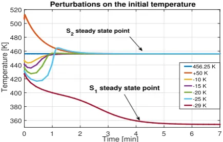
[image:6.595.312.531.373.512.2] [image:6.595.61.278.569.706.2]0 1 2 3 4 5 6 7
Time [min]
360 380 400 420 440 460 480 500 520
Temperature [K]
Perturbations on the initial temperature
456.25 K +50 K -10 K -15 K -20 K -25 K -29 K
S
2 steady state point
[image:7.595.56.274.55.194.2]S1 steady state point
Figure 8. Reactor’s temperature after perturbations on the reactant’s steady-state temperature.
0 1 2 3 4 5 6 7
Time [min] 0
0.2 0.4 0.6 0.8 1
Concentration [mol/l]
Perturbations on the initial temperature
456.25 K +50 K -10 K -15 K -20 K -25 K -29 K
S1 steady state point
[image:7.595.62.276.241.381.2]S2 steady state point
Figure 9. Reactor’s concentration after perturbations on the reactant’s steady-state temperature.
assumption which is only made for the analysis of the ideal situation.
The state-space differential equation for the linearized system is assumed to be in the form:
˙
x=Ax+Bu,x0=x(0) (11)
where x0 represents the vector of initial conditions. The performance index to be minimized represents an energy quantity which takes the following form
J(u, x0) =
Z ∞
0
(x(t)TQx(t) +u(t)TRu(t))dt (12)
If(A, B)is stabilizable and(A, Q)is detectable, the optimal solution to the regulator problem isu=Kx=−R−1BTP x
where P ≥0 is the stabilizing solution to the Algebraic Riccati Equation (ARE): ATP+P A−P BR−1BTP+
Q= 0. The static state-feedback control lawKxis applied to variations around the steady-state conditions and therefore is added to the steady-state control signals obtained via linearization. The weighting matricesQandRare tuned to shift the design emphasis between the penalizing of state and control variables, respectively. The initial choice of the weights can be calculated by the Bryson’s rule which specifies that the matricesQandRare diagonal with
Qii= 1
(xi,max)2 andRii=
1
(ui,max)2 (13)
where |xi,max| and |ui,max| are the maximum required values of the state and control variables, respectively. The
final values of Q and R are selected via a trial-and-error procedure which is guided by simulation results.
Fig. 8 shows the response of the plant when the initial condition in temperature is progressively decreased. As long as the temperature perturbation is less than 29 degrees the equilibrium of(456.25,0.0439)is recovered. When the initial condition is decreased by 29 degrees the temperature converges to the lower equilibrium point of354.23K. Fig.9 shows the analogous results for the concentration variable (for the same temperature perturbations). Fig. 10 and 11 show that by using the LQR controller, the initial equilibrium of (456.25,0.0439) can be recovered for the perturbation of ∆T =−29K. Three LQR designs are presented. The weights in the initial design are selected according to Bryson’s rule (Q= [1012 0; 0
1
0.04392], R= [
1 152 0; 0
1 202]).
In the other two designs the same Q matrix is used while the input penalty matrix Ris scaled by a positive factorσ
andσ1, respectively, whereσ= 2. Note that when the control effort is penalized heavily the closed-loop response becomes slower exhibiting larger overshoots. On the contrary, keeping the input penalty low results in faster recovery of the equilibrium point.
0 0.2 0.4 0.6 0.8 1 1.2 1.4 1.6 1.8 2
Time [min] 420
430 440 450 460
Temperature [K]
[image:7.595.318.530.336.475.2]Perturbation on initial temperature by -29K, = 2
Figure 10. Steady-state temperature recovery from 29 degree drop in initial temperature using three different tunings of the LQR controller.
0 0.2 0.4 0.6 0.8 1 1.2 1.4 1.6 1.8 2 Time [min]
0.05 0.1 0.15 0.2
Concentration [mol/l]
Perturbation on initial temperature by -29K, = 2
Figure 11. Steady-state concentration recovery from 29 degree drop in initial temperature using three different tunings of the LQR controller.
[image:7.595.315.530.547.685.2]Vlahakis and Halikias 7
concentration variable can not be measured at least in real-time as explained earlier. Hence, the overall design procedure should include an observer to estimate the reactor’s states. A higher-order controller is then constructed by combining this estimator with the state-feedback control law derived from the LQR method. Two complementary methods of obtaining an accurate estimate of the concentration measurement are discussed in the next section.
Robustness Properties
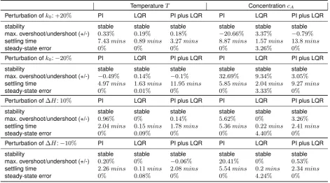
To assess the robustness properties of the control designs described in this section the following tests were performed. The reaction rate constantk0and the reaction heat∆Hwere perturbed by20% and 10%, respectively. The response of the nonlinear system with the three designed controllers (PI, LQR, PI plus LQR) is summarized in Table3. Note that in all three cases stability is maintained for these perturbations. Despite the fact that no integral action is used in the LQR control scheme the steady-state error in the concentration variable deteriorates by only4.40%. Naturally, when integral action is included in the controller (PI, PI plus LQR) the steady-state error is zero.
Concentration Estimation
The concentration measurement has proved beneficial for control design as typical input disturbances are rejected more efficiently and the reference steady-state working point is recovered. Recall that the concentration measurement is problematic due to the need to perform sample analysis which introduces unavoidable delays. The challenge here is to introduce estimation techniques which compensate for these delays and ideally get access to concentration’s actual value. For this purpose, a reduced-order observer and a future predictor are developed separately and a linear combination of those estimators is finally proposed.
Reduced-Order Observer
Considering theS2reactor’s working point, linear reduced-order observer is analyzed to estimate the concentration variation from temperature measurements. For that purpose, the non-linear set of differential equations of the reactor’s system is linearized around theS2 equilibrium point. The linearized equation is rewritten for convenience as
˙
x1
˙
x2
=
A11 A12
A21 A22
x1 x2
+
B11 B12
B21 B22
u1 u2
(14)
y=1 0
x1 x2
(15)
where x1 and x2 represent the deviation of temperature and concentration variables from the steady-state values, respectively, andu1andu2account for the deviation of the inputs from the steady-state values. With respect to theS2 working point the linearized dynamics and input matrices are given in eq. (9).yrepresents the output of the linearized model which corresponds to the measured state. Therefore, onlyx2(t)is estimated and the linearized equations are now written as:
˙
x2=A22x2+ ˜Bu˜ (16)
where B˜ ,
A21 B21 B22 and u˜,
x1 u1 u2
=
y u1 u2
which is a known signal. Also, the signal
˜
y,x˙1−A11x1−B11u1−B12u2=A12x2 (17)
is known. An observer forx2can now be constructed as
˙ˆ
x2= (A22−KA˜ 12)ˆx2+ ˜Bu˜+ ˜Ky˜ (18)
In order to eliminatex˙1in they˜equation, letwbe defined asw= ˆx2−Ky˜ and obtain from (18) an estimate in terms ofw,y,u1andu2. In particular,
˙
w= (A22−KA˜ 12)w
+ [(A22−KA˜ 12) ˜K+A21−KA˜ 11]y
+hB
21−KB˜ 11 ... B22−KB˜ 12 iu1
u2
(19)
Then w+ ˜Ky is an estimate for xˆ2 and the concentration variable can be estimated as:
ˆ
cA=w+ ˜Ky+csA (20)
wherecs
Ais the steady-state value. Notice that the error signal e(t) =x2−xˆ2satisfies the equation
˙
e= ˙x2−x˙ˆ2= (A22−KA˜ 12)e (21)
and if the pair(A22, A12)is observable, then the eigenvalues of A22−KA˜ 12 can be arbitrarily assigned via K˜. In this case, sinceA22andA12are scalar the eigenvalue assignment is possible if A126= 0. In the case that A12= 0, A22 should be negative in order for the error e to converge to zero asymptotically. It should be noticed that in the case of a linear plant, absence of model uncertainty and assuming that neither the input nor the output channels are corrupted by noise, the observer in theory can be constructed arbitrarily fast with appropriate selection ofK˜. In the present application where the dynamics are strongly non-linear, additional attention should be paid to the selection of the gain
˜
K.
Regarding the observer’s structure, the signal y˜ may be corrupted by noise arising in the temperature sensor. This is further amplified after numerical differentiation when signal
˜
y is constructed. Therefore, it makes sense to limit noise amplification via low-pass filtering.
Concentration Predictor
Typically the concentration measurement is obtained by sample analysis assumed to be completed within time interval δτ. We also assume that the measurement process is implemented periodically and thus it is modelled as a discrete-time process. The measurements then take the form
y1[k] y2[k]
=
T[k]
cA[k−δτ]
(22)
where the delayδτis considered to be an integer multiple of the sampling interval of the system. The idea is to design a predictor which projects the delayed measurements into the
Table 3. Stability and time characteristics of the reactor’s temperatureTand molar concentrationcAconsidering perturbations on
the reaction rate constantk0and the reaction heat∆Hfor three different control schemes.
TemperatureT ConcentrationcA
Perturbation ofk0:+20% PI LQR PI plus LQR PI LQR PI plus LQR
stability stable stable stable stable stable stable
max. overshoot/undershoot (+/-) 0.33% 0.19% 0.18% −20.66% 3.37% −0.79% settling time 7.43mins 0.89mins 3.27mins 8.87mins 1.57mins 13.8mins
steady-state error 0% 0% 0% 0% 3.26% 0%
Perturbation ofk0:−20% PI LQR PI plus LQR PI LQR PI plus LQR
stability stable stable stable stable stable stable
max. overshoot/undershoot (+/-) −0.49% 0.14% −0.1% 32.69% 9.34% 3.05% settling time 4.97mins 1.63mins 11.95mins 5.85mins 2.04mins 9.27mins
steady-state error 0% 0.01% 0% 0% 3.33% 0%
Perturbation of∆H:10% PI LQR PI plus LQR PI LQR PI plus LQR
stability stable stable stable stable stable stable
max. overshoot/undershoot (+/-) 0.96% 0% 0.14% 5.62% 0% 3.26%
settling time 2.04mins 0.15mins 1.78mins 5.36mins 0.22mins 2.41mins
steady-state error 0% 0.09% 0% 0% 4.40% 0%
Perturbation of∆H:−10% PI LQR PI plus LQR PI LQR PI plus LQR
stability stable stable stable stable stable stable
max. overshoot/undershoot (+/-) 0.20% 0% −0.06% 20.41% 0% 0.53%
settling time 2.26mins 0.11mins 2.08mins 5.54mins 0.2mins 2.34mins
steady-state error 0% 0.08% 0% 0% 4.24% 0%
future. Here a discrete-time linear predictor is first analyzed which is then extended to a nonlinear predictor. It is also assumed that the system is linearized around the stable equilibrium point and the discrete model is obtained as the zero-order-hold equivalent of the continuous time process. The difference equations for the linearized plant at thek-th sampling instance can be written as
x1[k] x2[k]
=
Ad11 Ad12
Ad21 Ad22
x1[k−1] x2[k−1]
+
Bd11 Bd12
Bd21 Bd22
u1[k−1] u2[k−1]
(23)
y1[k] y2[k]
=
x1[k] x2[k−n]
(24)
where n= δτt
s. For sampling time ts= 0.25 min the above dynamics (Ad) and input (Bd) matrices are found
1.011 208.4
−0.002 −0.431
and
0.137 −0.310 0.0002 0.0005
respectively.
Hence, the deviation in temperature from its set-point,x1, is accessible in almost real time (actually with a delay of one sampling interval) while the deviation in the concentration variable x2 is accessible only after n sampling periods. Solving forx2we get
x2[k] =Ad21x1[k−1] +Ad22x2[k−1]
+Bd21u1[k−1] +Bd22u2[k−1]
=Adn22x2[k−n]+ (25)
+
n X
j=1
Adj−221
Ad21 Bd21 Bd22
x1[k−j] u1[k−j] u2[k−j]
A future predictor forx2can now be constructed as
¯
x2[k] =Adn22x¯2[k−n] + n X
j−1
Adj−221B¯u¯[k−j] (26)
where
¯
B=Ad21 Bd21 Bd22
andu¯[k−j] =
x1[k−j] u1[k−j] u2[k−j]
.
A prediction for the concentration value at time instantkis given by
¯
cA[k] = ¯x2[k] +csA (27)
Note that if the model is accurate and the input and output signals are noise-free, the predictor x¯2 is expected to converge to x2 even in the case |Ad22|>1 provided the delay interval is sufficiently short. When the model is corrupted by uncertainties or the input and output channels are noisy, it may be helpful to augment the predictor’s equation with an innovations signal amplified by a gain
K to guarantee that the errore=x2[k]−x¯2[k] converges asymptotically to zero.
The construction is now extended to a nonlinear predictor. In this case, there is no need for linearization and the discrete-time non-linear model of the reactor takes the form
x1[k] x2[k]
=
f(x1[k−1], x2[k−1], u[k−1]) g(x2[k−1], x1[k−1], u[k−1])
(28)
y1[k] y2[k]
=
x1[k] x2[k−n]
(29)
A nonlinear predictor ofx2[k]can be constructed recursively as:
ˆ
x2[k] =g(ˆx2[k−1], x1[k−1], u[k−1]) (30)
ˆ
x2[k−1] =g(ˆx2[k−2], x1[k−2], u[k−2]) (31)
.. .
ˆ
x2[k−n+ 1] =g(ˆx2[k−n], x1[k−n], u[k−n]) (32)
ˆ
Vlahakis and Halikias 9
If the functions f and g describe the reactor’s model accurately and the delay interval is not excessively long,
ˆ
x2[k]is expected to predictx2[k]with acceptable accuracy as can be tested experimentally or in simulation environment.
Combined Estimator
A reduced-order observer and a predictor have been pro-posed to obtain independent estimates of the concentration variable. When sample analysis is not available, the observer design may be the solution to the estimation problem. In cases where a delayed concentration measurement is avail-able, real-time concentration may be estimated via future predictor and as a result two estimates are available to the designer to decide upon the concentration value. A linear combination of reduced-order observer and linear predictor can be used to produce a combined estimate which can then be used for state-feedback control design purposes. As the observer is in continuous time we need to discretize the observer signal so that the outputs of both estimators can be combined. In particular, letˆcAbe the observer’s signal after
the zero-order-hold andc¯Abe the predictor’s output. Then,
the overall concentration estimate˜cAis defined as
˜
cA=λˆcA+ (1−λ)¯cA (34)
where λ∈[0,1]. Parameter λ can be used to shift the emphasis between the two estimation methods to reflect the relative accuracy of each scheme. For example, when the reactor’s parameters are highly uncertain the value of
λshould be selected low (between 0 and 1) so that more emphasis is placed on the predictor’s estimate. In contrast, when the sample analysis results are poor the value of λ
should shift in the opposite direction.
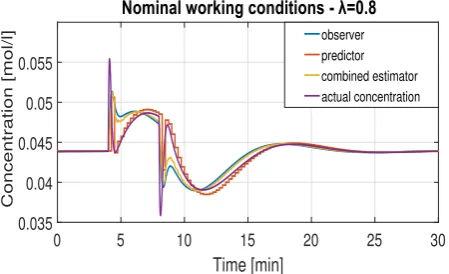
Fig. 12, 13 and 14, 15 show the time response of the concentration signals (actual, estimates) for two values of λ under nominal and perturbed working conditions, respectively. LQR and PI controllers fed by temperature measurements and concentration estimates have been designed to reject pulse disturbances in the feeder. Figures12 to15illustrate that the three estimates with the observer, the predictor and the combined estimator converge to the true state under both nominal and perturbed working conditions with acceptable transient response. In particular, it should be noted that the reduced-order observer estimates the actual concentration variable with acceptable accuracy in the absence of input disturbances while the predictor tracks the actual value even if the input signals are corrupted by external interference.
Conclusion
Control techniques for exothermic chemical reactions taking place in continuous stirred tank reactor were investigated. The dynamic characteristics of the nonlinear system were analyzed and several control schemes (PI, LQR) were proposed and assessed via extensive simulations. The problematic nature of the real-time measurement of the molar concentration variable was highlighted and motivated our investigation into effective estimation techniques for CSTR systems which are subject to measurement delays. A linear reduced-order observer was then proposed and
0 5 10 15 20 25 30
Time [min]
0.03 0.035 0.04 0.045 0.05 0.055 0.06
Concentration [mol/l]
[image:10.595.307.531.57.198.2]observer predictor combined estimator actual concentration
Figure 12. Nominal working conditions, concentration signals forλ= 0.5.
0 5 10 15 20 25 30
Time [min]
0.035 0.04 0.045 0.05 0.055
Concentration [mol/l]
[image:10.595.307.532.246.383.2]observer predictor combined estimator actual concentration
Figure 13. Nominal working conditions, concentration signals forλ= 0.8.
0 5 10 15
Time [min]
0.02 0.04 0.06 0.08 0.1 0.12
Concentration [mol/l]
observer predictor combined estimator actual concentration
Figure 14. Perturbed working conditions, concentration signals forλ= 0.5.
used to estimate molar concentration value from temperature measurements and discrete-time linear and a non-linear predictor was constructed via an iterative process. By applying the separation principle, the estimator obtained by these two methods, combined with optimal state-feedback and PI control can lead to a dynamic controller and solve the regulation problem for the reactor system. Further work is needed, however, to ensure that the control schemes obtained in this way have adequate stability margins and can therefore be implemented successfully in practical applications.
Declaration of conflicting interests
The Authors declare that there is no conflict of interest.
[image:10.595.310.531.432.569.2]0 5 10 15
Time [min]
0.02 0.04 0.06 0.08 0.1 0.12
Concentration [mol/l]
[image:11.595.58.279.57.195.2]observer predictor combined estimator actual concentration
Figure 15. Perturbed working conditions, concentration signals forλ= 0.8.
Funding
This work was carried out in the framework of the GLOW Project - New weather-stable low gloss powder coatings based on bifunctional acrylic solid resins and nanoadditives - funded by the European Commission Seventh Framework Programme (FP7/2007-2013) under Grant Agreement No. 324410.
References
Antonelli R and Astolfi A (2003) Continuous stirred tank reactors: Easy to stabilise? Automatica39(10): 1817–1827.
Bakeev KA (2005)Process Analytical Technology. 2nd edition. West Sussex, UK: John Wiley & Sons, Ltd.
Banu US and Uma G (2008) Fuzzy Gain Scheduled Continuous Stirred Tank Reactor with Differential Evolution Based PID Control Minimizing Integral Square Error. Instrum. Sci. Technol.36: 394–409.
Barkhordari Yazdi M and Jahed-Motlagh MR (2009) Stabilization of a CSTR with two arbitrarily switching modes using modal state feedback linearization.Chem. Eng. J.155(3): 838–843. Baruah S and Dewan L (2017) A comparative study of PID based
temperature control of CSTR using Genetic Algorithm and Particle Swarm Optimization. In: 2017 Int. Conf. Emerg. Trends Comput. Commun. Technol.
Botero H and ´Alvarez H (2011) Non Linear State and Parameters Estimation in Chemical Processes: Analysis and Improvement of Three Estimation Structures Applied to a CSTR. Int. J. Chem. React. Eng.
Gao R, O’dywer A and Coyle E (2002) A nonlinear PID controller for CSTR using local model networks. Proc. 4th World Congr. Intell. Control Autom.: 3278–3282.
Guay M, Dier R, Hahn J and McLellan PJ (2005) Effect of process nonlinearity on linear quadratic regulator performance. J. Process Control15(1): 113–124.
Hofmann A (2010) Spectroscopic Techniques: I Spectrophotomet-ric Techniques. In:Princ. Tech. Biochem. Mol. Biol.Cambridge University Press.
Ingham J, Dunn IJ, Prenosil JE, Heinzle E and Snape JB (2007) Chemical Engineering Dynamics: An Introduction to Modelling and Computer Simulation. Third edition. Weinheim: WILEY-VCH.
Jouili K, Charfeddine S and Jerbi H (2008) An advanced geometric approach of input-output linearization for nonlinear control of
a CSTR. In:Proc. - EMS 2008, Eur. Model. Symp. 2nd UKSim Eur. Symp. Comput. Model. Simul.pp. 353–358.
Kim M, Lee YH and Han C (2000) Real-time classification of petroleum products using near-infrared spectra. Comput. Chem. Eng.24(2-7): 513–517.
Komari Alaei H and Yazdizadeh A (2014) Robust flow controller design and analysis for a chemical process. Trans. Inst. Meas. Control36(6): 723–733.
Kravaris C, Hahn J and Chu Y (2013) Advances and selected recent developments in state and parameter estimation. Comput. Chem. Eng.51: 111–123.
Krishnan A, Patil B, Nataraj P, Maciejowski J and Ling K (2017) Model predictive control of a CSTR: A comparative study among linear and nonlinear model approaches. In:2017 Indian Control Conf. ICC 2017 - Proc.
Kvasnica M, Herceg M, Cirka L and Fikar M (2010) Model predictive control of a CSTR: A hybrid modeling approach. Chem. Pap.64(3): 301–309.
Li DJ (2013) Adaptive neural network control for continuous stirred tank reactor process. In:IFAC Proc. Vol., volume 3. pp. 171– 175.
Mayne DQ (2014) Model predictive control: Recent developments and future promise.Automatica50(12): 2967–2986.
Mohd Ali J, Ha Hoang N, Hussain MA and Dochain D (2015) Review and classification of recent observers applied in chemical process systems.Comput. Chem. Eng.76: 27–41. Naifar O, Ben Makhlouf A, Hammami MA and Ouali A (2016) On
Observer Design for a Class of Nonlinear Systems Including Unknown Time-Delay.Mediterr. J. Math.13(5): 2841–2851. Oravec J and Bakoˇsov´a M (2015) Robust model-based predictive
control of exothermic chemical reactor. Chem. Pap.69(10): 1389–1394.
Santos AF, Silva FM, Lenzi MK and Pinto JC (2005) Monitoring and Control of Polymerization Reactors Using NIR Spectroscopy.Polym. Plast. Technol. Eng.44(1): 1–61. Shakeri E, Latif-Shabgahi G and Abharian AE (2017) Design
of an intelligent stochastic model predictive controller for a continuous stirred tank reactor through a Fokker-Planck observer. Trans. Inst. Meas. Control.
Tofighi S, Bayat F and Merrikh-Bayat F (2017) Robust feedback linearization of an isothermal continuous stirred tank reactor: H mixed-sensitivity synthesis and DK-iteration approaches. Trans. Inst. Meas. Control39(3): 344–351.
Vasiˇckaninov´a A and Bakoˇsov´a M (2009) Neural Network Predictive Control of a Chemical Reactor. In: Control, volume 2. pp. 21–36.
Vasiˇckaninov´a A, Bakoˇsov´a M, ˇCirka L and Kal´uz M (2015) Comparison of robust control techniques for use in continuous stirred tank reactor control. IFAC-PapersOnLine28(14): 284– 289.
Vojtesek J and Dostal P (2011) MATLAB program for Simulation and Control of the Continuous Stirred Tank Reactor. Recent Res. Circuits, Syst. Signal Process.: 45–50.