Optimal detection and error exponents for hidden semi-Markov models

Optimal detection and error exponents for hidden

semi-Markov models

Dragana Bajovi´c, Kanghang He, Lina Stankovi´c, Dejan Vukobratovi´c, and Vladimir Stankovi´c

1

Abstract. We study detection of random signals corrupted by noise that over time switch their values (states) between a finite set of possible values, where the switchings occur at unknown points in time. We model such signals as hidden semi-Markov signals (HSMS), which generalize classical Markov chains by introducing explicit (possibly non-geometric) distribution for the time spent in each state. Assuming two possible signal states and Gaussian noise, we derive optimal likelihood ratio test and show that it has a computationally tractable form of a matrix product, with the number of matrices involved in the product being the number of process observations. The product matrices are independent and identically distributed, constructed by a simple measurement modulation of the sparse semi-Markov model transition matrix that we define in the paper. Using this result, we show that the Neyman-Pearson error exponent is equal to the top Lyapunov exponent for the corresponding random matrices. Using theory of large deviations, we derive a lower bound on the error exponent. Finally, we show that this bound is tight by means of numerical simulations.

Keywords. Multi-state processes, hidden semi Markov mod-els, explicit random duration, hypothesis testing, error expo-nent, large deviations principle, threshold effect, Lyapunov exponent.

I. INTRODUCTION

The problem of detecting a signal hidden in noise is inves-tigated. The signal to be detected is characterised as having a constant magnitude in any one state and can transition to multiple states over time. Each occurrence of a particular state has a random duration, modelled as a discrete random variable which takes values from the finite set of integers, according to a certain probability mass function (pmf) associated with that state. Signal models of this kind are known in the literature as hidden semi-Markov models (HSMM) [1][2], which differ from the standard hidden Markov models in that in each state, the process can emit more than one observation. The underlying unobservable process in this case is called semi-Markov [3], and is defined as a sequence of pairs of two random variables – one from the Markov chain evolving

1_{D. Bajovic and D. Vukobratovic are with Department of Power, Electronic}

and Communications Engineering, Faculty of Technical Sciences, University of Novi Sad, Novi Sad, Serbia (e-mail: {dbajovic, [email protected]}) K. He, L. Stankovic and V. Stankovic are with Department of Electronic and Electrical Engineering, University of Strathclyde, Glasgow, G1 1XW, UK (e-mail:{kanghang.he, lina.stankovic, vladimir.stankovic}@strath.ac.uk)

sequence of states, and the other being the time spent in each visited state, the statistics of which is described by a pmf (or pdf, in the continuous time case). A related, more general class of random multi-state signals are Markov switching models [4] (or Markov jump processes) generally used to model time series and other kinds of signals, where the signal parameters of a certain model (e.g., moving average [4]) switch over time in a Markov fashion. When the durations of each parameter regime are modelled explicitly by a pmf (or pdf), the corresponding model is called explicit-duration Markov switching models – of which HSMMs are a special case.

Our main motivation for studying the described model comes from non intrusive appliance load monitoring (NILM) problem, i.e., detecting one or more particular appliance states, each of unknown duration, within an aggregate power signal, as obtained from smart meters. With the large-scale roll-out of smart meters worldwide, there has been increased interest in NILM, i.e., disaggregating total household energy consumption measured by the smart meter down to appliance level using purely software tools [5]. NILM can enrich energy feedback, it can support smart home automation [6], appliance retrofit decisions, and demand response measures [7].

NILM is an NP-hard problem [5], and an exact solution can only be found via exhaustive search: in practice, it would take over 1700 years to disaggregate 30 appliances using exhaustive search from a months data with top current GPUs [8, p. 124]. Since NILM boils down to identifying unknown sources that go through a sequence of (hidden) states (ON to OFF for single state loads), Hidden Markov Models (HMM), have become popular for this time-series data, with a number of extensions proposed over the past few years, including factorial HMM (FHMM), conditional FHMM, etc. [9], [10], [11], [12]. How-ever some appliances violate the Markovian assumption [8, p.142], as the durations that appliances are on and off are not geometrically distributed, as occurs with HMMs. Further, the duration of appliance runs are not captured, which is the key difference w.r.t speech applications where durations of sounds are approximately equal.

Processing (GSP) [15], [16], Decision Trees [7], particle filter-ing, evolutionary algorithms [17], etc., but without measurable and convincing evidence of reliability, acceptable accuracy, and scalability.

Despite significant research efforts in developing efficient NILM algorithms (see [7], [15], [16], [9], [10] and references therein), NILM is still a challenge, especially at low sampling rates, in the order of seconds and minutes. One obstacle is the lack of standardised performance measures and appropriate theoretical bounds of detectability of appliance usage, which can help estimating performance of various algorithms. A particularly challenging problem is the detection of multi-state appliances, i.e., appliances whose power consumption switches over one appliance runtime through several different values. Examples of such appliances are a dishwasher or a washing machine, where the load or the chosen program or setting determines duration that the appliance spends in each state. The difficulty there arises from the fact that the program and the load, unknown from the perspective of NILM, are non-deterministic, i.e., vary each time the same appliance is run resulting in difficulty in detecting in which state the appliance is. In this work we propose to use HSMM as a model for multi-state appliances, where we have the full freedom to describe the state durations statistics, and thus obtain a better fit for multi-state appliance signals than with HMMs, which allow only for geometrically decaying pmfs on the state durations. The aggregate load minus the load of the appliance to be detected, consisting of other appliances being switched on and off randomly over time, is well modelled as Gaussian additive noise, as shown in [11].

HSMM is also representative of signals occurring in a range of other applications. In econometrics, examples of explicit duration signals include marital or employment status, or in general the time an individual spends in a certain state [18]. Further examples from econometrics are time to currency alignment or time to transactions in stock market [19]. In biometrics, HSMM is used to model forest tree growth and identify individual growth components [20]. In communication systems theory, pulse-duration modulated (PDM) signals for transmitting information encoded into the pulse duration have two possible signal states: the positive value state is a pulse whose duration is proportional to the information symbol to be encoded, and the zero-value state in between any two pulses. The probability distribution of the state duration is then con-trolled by the probability distribution on the set of information symbols to be transmitted. Further binary state examples are random telegraph signals, where the signal switches between two values in a random manner2, and the activity pattern of a certain mobile user in a cellular communication system. We refer the reader to references [2], [4], [1] for detailed accounts on various other applications of HSMMs.

In this paper we focus on detection of binary signals of random state durations, hidden in noise, modelled as (binary) HSMMs. While the problem of detecting multi-state signals hidden in noise has been presented in [21], [23] and [24],

2_{We remark that there are other stochastic models in the literature for the}

random telegraph signal, e.g., the Poisson model, or the hidden Markov chain model [21], [22].

the latter model the signal as hidden Markov chains unlike our proposed approach which adopts HSMM, with an explicit duration model for each of the states. Specifically, in [21] random telegraph signals are modelled as binary Markov chains and the corresponding optimal detection test is derived in the form of a product of certain measurement defined matrices. Detection of a random walk on a graph is considered in [23], where bounds on the error exponent for the Neyman-Pearson detection test are derived. The method of types is used in [24] to generalize the results from [23] to non-homogeneous setting where different nodes have different signal-to-noise ratios (SNR) with respect to the walk. Furthermore, proof is given in [24] that the derived bound on the error exponent has a convex optimization form.

Assuming Neyman-Pearson setting, we are interested in detection performance characterization, through computing the corresponding error exponent – the decay rate of the probability of a miss, under a constraint on the probability of false alarm, for given HSMM model parameters. It is well-known that when observations are independent and identically distributed (i.i.d.) both in the presence and absence of the signal (e.g., when the signal value is constant and known and the noise realizations are i.i.d.), the Neyman-Pearson error exponent is given by the Kullback-Leibler divergence between the corresponding two hypotheses, see Stein’s lemma in [25], [26], and also [27]. This property, in a sense, extends to non-i.i.d. signal models of certain classes (such as, for example, ergodic models), in which case the error exponent is given by the asymptotic Kullback-Leibler rate [28], [29] (see the expression in (7) in Section II further ahead). Computing this limit is a difficult problem in general, but, for certain cases, solutions are known.

We briefly review the literature on error exponents for signals with Markovian structure. In [30] error exponent is computed for testing between two different Markov sources (without additive noise in the observations); for applica-tions and extensions of this result in Markov source-coding see [31], [32], [33], [34]. Error exponents for HMMs are considered in [23] and [24], as detailed above. Error exponent is also shown to be computable for the problem of discrimi-nating between two autoregressive processes (AR) of different parameters [35], [36]. For Gauss-Markov models, represented as AR process of order 1 with Gaussian noise, [37] finds a closed form for the error exponent via spectral domain characterization of the observed process. To the best of our knowledge, there are no results on the error exponent for HSMMs.

diagonal random matrix controlled by the process observations and a sparse constant matrix which governs transitions in the sequence of states of different durations. Thus, we reveal that a similar structural effect as with the error exponent for hidden Markov processes occurs here as well [21], [24]. This result is of immediate interest for inference in HSMM, as it allows extension and application to HSMM of certain algorithms designed for HMM that specifically rely on matrix product representation of the likelihood, see [20], [39]. Further, using the introduced transition matrix for the semi-Markov model, we find explicitly an upper bound on the error exponent, equal to the expected SNR of the process. This bound has an intuitive physical interpretation: it is the error exponent for the detection test which has information on the exact locations of all state transitions in the observed sequence of measurements. Finally, using the theory of large deviations [26], we derive a lower bound on the error exponent and demonstrate by numerical simulations that the derived bound is very close to the true error exponent.

Paper outline. Section II states the problem setup and Sec-tion III gives the preliminaries. SecSec-tion IV gives main results on the form of the optimal likelihood ratio test. Section V provides the lower bound on the error exponent, while Sec-tion VI proves this result. Finally, numerical results are given in Section VII and Section VIII concludes the paper.

Notation. For an arbitrary integer n,Sn−1 _{denotes the} prob-ability simplex in Rn_{; e1 denotes the first canonical vector}

(the n dimensional vector with 1 only in the first position, and having zeros in all other positions), and 1 the vector of all ones, where we remark that the dimension should be clear from the context; A0 denotes the lower shift matrix (the 0/1

matrix with ones only on the first subdiagonal); k · kdenotes the spectral norm. We denote Gaussian distribution of mean value µand standard deviation σ byN(µ, σ2); byp[1, n] an arbitrary distribution over the first n integers; by U[1, n] the uniform distribution over the first nintegers; log denotes the natural logarithm.

II. PROBLEM SETUP

We consider the problem of detecting a signal corrupted by noise that randomly switches from one state m to another, where m = 1,2, ..., M and in each state the signal has a certain magnitude µm. The duration that the signal spends in

a given state mis modelled as a discrete random variable on a given support set [1,∆m], and with a certain pmf defined

by vector pm ∈ S∆m−1. In this work, we consider the case

when M = 2and we assume that for each statemwe know the corresponding value of the observed signal µm. Without

loss of generality, we will assume that µ2 > µ1 ≥ 0. For each sampling time t = 1,2, ..., let St_{={S1, ..., S}

t} denote

the sequence of states until time t of the signal that we wish to detect, where for each k= 1, ..., t, Sk ∈ {1,2}; similarly,

we denote S∞ ={S1, S2, ...}. Let also St _{denote the set of}

all feasible sequences of states st of length t. We assume that, with probability one, the first state is S1 ≡ 1, and, for the purpose of analysis, we set S0 ≡ 2. Let Xk denote

the signal measurement for sample time k, k= 1, ..., t, and, for each t, collect all measurements up to time t in vector Xt _{= (X}

1, ..., Xt). We assume that each measurement is

corrupted by a zero mean additive Gaussian noise N(0, σ2_), where standard deviationσ >0.

The sequence of switching times.For the sequence of states S1, S2, ..., we define the sequence of times{T1, T2, ...}, when the signal in the sequence switches from one state to another, i.e.,

Ti+1= max{k≥Ti+ 1 :Sk=STi+1}, fori= 0,1,2, ... (1) where we set T0 ≡ 0. We call a phase each time window

[Ti+ 1, Ti+1],i= 0,1,2, . . ., and note that during any phase, the sequence S∞ stays in the same state. Since S1 ≡1, all odd-numbered intervals [T0 + 1, T1], [T2 + 1, T3],..., where the ordering is with respect to the order of appearance, are state 1 phases, and all even-numbered intervals [T1+ 1, T2],

[T3+ 1, T4],... are state2phases.

Random duration model. For n = 1,2, ..., we denote by D1,n the difference process

D1,n=T2n−1−T2n−2, (2)

or, in words, for eachn,D1,nis the duration of then-th state-1

phase in the sequenceS∞. We assume that durations of state-1

phases are independent and identically distributed (i.i.d.), with support set of all integers in the finite interval[1,∆1], and with pmf given by vectorp1= (p11, p12, ..., p1∆1)∈S

∆1−1_{, which} we denote byD1,n∼p1(1,∆1). Similarly, we define

D2,n=T2n−T2n−1 (3)

to be the duration of the n-th state-2 phase in the sequence S1, S2, ..., for n = 1,2, ...; we assume that the D2,n’s are

i.i.d., with support set of all integers in the interval[1,∆2], and pmf given by vector p2 = (p21, p22, ..., p2∆₂)∈ S∆2−1_{, i.e.,} D2,n ∼p2(1,∆2). We also assume that durations of state-1 and state-2 phases are mutually independent.

Hypothesis testing problem.Using the preceding definitions, we model the signal detection problem as the following binary hypothesis testing problem:

H0:Xk

i.i.d.

∼ N(0, σ2) (4)

H1:Xk|St

indep.

∼

N(µ1, σ2), ifSk = 1

N(µ2, σ2), ifSk = 2

,fork= 1, ..., t,

where we assume S1 ≡ 1. We remark that the model above easily generalizes to the case when the signalsXk are

under both hypotheses shifted for some µ0 ∈ R, i.e., when, under H = H0, Xk ∼ N(µ0, σ2) and, under H = H1,

Xk ∼ N(µSk+µ0, σ

2_{); see the example of appliance detection} problem later in this section. The latter hypothesis testing problem reduces to the one in (4) by means of the change of variablesYk =Xk−µ0.

whose signature signals exhibit a multistate (multiphase) type of behavior, such as switching from high to low signal values, where the durations of phases of the same signal level can be different across a single appliance run-time and also in differ-ent run-times of the same appliance. Examples of appliances whose signatures fall into this class are, e.g., a dishwasher and a washer-dryer. This problem can be modelled by the hypothesis testing problem (4) where µ1 corresponds to the appliance consumption when in low state andµ2 corresponds to the appliance consumption when in high state. In this scenario, there is an underlying baseline load which can also be modelled as a Gaussian random variable of expected value µ0 and standard deviationσ2. Since the same baseline load is present both underH0andH1, to cast the described appliance detection problem in the format given in (4), we simply subtract the value µ0 from the observed consumption signal Xk.

Comparison with random telegraph signals. The signal model that we consider is structurally similar to the random telegraph signal, modelled as a hidden binary Markov chain. The random telegraph signal switches between two opposite signal values, µ1 = +µand µ2 =−µ, where the transitions are governed by a certain transition matrix, which we denote by PRT = [q (1−q); (1−q)q] (assuming, for simplicity, symmetry in the two states). Given that the random telegraph signal has just entered, say, state1, we look at the probability that the signal stays in this state for d time instants, where d is arbitrary. It is easy to show that this probability equals

(1−q)qd−1_{, for arbitrary d ≥ 1. That is, with the random} telegraph signal, the distribution on the durations of states is geometric – thus, it decays withdexponentially. On the other hand, with the binary semi-Markov model that we consider, there is a complete freedom in setting the distribution on the time that the signal spends in either of the states, provided that the maximal state duration is bounded by some finite∆. When

∆ is large, and these pmfs are quasi (truncated) geometric, p1 =p2 = 1/(1−q∆) 1−q, q(1−q), . . . , q(1−q)∆−1, the semi-Markov model can be approximated by the random telegraph signal, which has a simpler parametric representa-tion. However, when the two pmfs are, for example, uniform, or even when the longer state durations in the studied signal are much more likely than the shorter ones (consider p1 = p2= (, , . . . , 1−(∆−1))), then the semi-Markov model is a much better alternative to the random telegraph signal. With multi-state appliances, once entered, any state is likely to last for a certain time (usually much longer than the unit, sampling period time), and hence the motivation to use semi-Markov models over semi-Markov chains. See also Section VII and Figure 8 for a numerical illustration of the comparison of the two models.

Likelihood ratio test and Neyman-Pearson error exponent. We denote the probability laws corresponding to H0 andH1 by P0 and P1, respectively. Similarly, the expectations with respect toP0andP1 are denoted byE0andE1, respectively. The probability density functions of Xt under H1 and H0 are denoted by f1,t(·) and f0,t(·), respectively. It will also

be of interest to introduce the conditional probability density function ofXt _givenSt_=st _{(i.e., the likelihood functions),}

which we denote by f1,t|St(·|st), for any st. Finally, the likelihood ratio at time t denoted by Lt, and at a given

realization ofXt_{is computed by L}

t(Xt) =f1,t(X

t₎

f0,t(Xt). It is well known that the optimal detection test (both in Neyman-Pearson and Bayes sense) for problem (4) is the likelihood ratio test. Conditioning on the state realizations until timet,St_=st_{, and denoting shortly P(s}t_{) =P1(S}t_=st_),

we have

Lt(Xt) =

X

st_∈St

P(st)f1,t|St(X

t_|st₎

f0,t(Xt)

= X

st_∈St P(st)

Qt

k=1 1

√

2πσe

−(µsk−Xk)2

2σ2

Qt

k=1 1

√

2πσe −Xk2

2σ2

, (5)

where, we recall,St _{is the set of all feasible sequences – for}

which P1(St _=st_{) >0. In this paper our goal is to find a}

computationally tractable form for the optimal, likelihood ratio test and also to characterize its asymptotic performance, when the number of samples Xk grows large. In particular, with

respect to performance characterization, we wish to compute the error exponent for the probability of a miss, under a given bound αon the probability of false alarm:

lim

t→+∞−

1

tlogP

α

miss,t=:ζ, (6)

whereP_missα _,t is the minimal probability of a miss among all decision tests that have probability of false alarm bounded byα. By results from detection theory, e.g., [28], [29], theζ in (6) is given by the asymptotic Kullback-Leibler rate in (7), provided that this limit exists

ζ= lim

t→+∞−

1

t logLt(X

t_{). (7)}

Fig. 1: Simulation setup: ∆ = 3, p1, p2 ∼ U([1,∆]), µ1 = 2, µ2 = 5, σ = 10, α = 0.01. Green full line plots the evolution of−1

tlogLt; blue dotted line plots the evolution of

−1

tlogP α

miss,t, and red dashed line plots the estimated slope

of the probability of a miss values (in the logarithmic scale) calculated for values untilt= 300observations.

−1

tlogP α

miss,t and −1tlogLt(X

t_{) are convergent and}

more-over that they converge to the same value – the asymptotic Kullback-Leibler rate for the two hypotheses defined in (4). For further details on this simulation see Section VII.

III. PRELIMINARIES

In this section we now introduce a number of quantities related with the sequences st _{∈ S}t_{, t = 1,2, ..., and give}

certain results pertaining to these quantities that will be useful for our analysis.

Statistics for the durations of phases. For each t, for eachst_{, we introduceN}

1 andN2 to count the number of state-1 and state-2 phases, respectively, in the sequencest_:

N1(st) =|{1≤k≤t: sk−1= 2, sk= 1}| (8)

N2(st) =|{1≤k≤t: sk−1= 1, sk= 2}|, (9)

where, since the first phase is state-1 phase, we set s0 ≡2. Note that functions N1 andN2 are, strictly speaking, depen-dent on time t (this dependence is observed in their domain sets St _{which clearly change with time t). However, for}

reasons of easier readibility, we suppress this dependence in the notation, as we also do for all the subsequently defined quantities. We remark that, for any sequence st_{, if the last}

state st = 2, then N1(st) = N2(st), and if st = 1, then

N1(st_{) = N2(s}t_{) + 1. Finally, N(s}t_{) is the total number of}

phases inst_,N≡N1+N2.

We further define the setsTmn(st)that contain time indices

for the n-th state-m phase, n = 1, ..., Nm(st),m = 1,2; to

compactly express the likelihood ratio (see expression (27) further ahead), it will also be of interest to group the Tm,ns

toTm(st) :=∪ Nm(st)

n=1 Tmn(st), with its cardinality denoted by

τm(st), form= 1,2. We now go over each state phaseTm,n,

m= 1,2, and increase the counter corresponding to this phase duration,d=|Tm,n|,

N1d(st) = N1(st)

X

n=1

1{|T1n|=d}(s

t_{), ford= 1, ...,∆}

1, (10)

N2d(st) = N2(st)

X

n=1

1{|T2n|=d}(s

t_{), ford= 1, ...,∆}

2; (11)

i.e., in words, vectors (Nm1, ..., Nm∆m),m= 1,2, represent histograms of phase1and phase 2durations. It is easy to see that Nm =P

∆m

d=1Nmd, for m= 1,2. Also, for each time t

and each sequence st, the total number of state1 and state 2

occurrences must sum up tot, and thereforeP∆1

d=1d N1d(st)+

P∆2

d=1d N2d(st) =t.

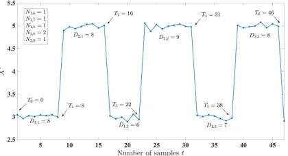
Figure 2 shows an example of simulation signals under Hypothesis H1 with ∆1 = ∆2 = 10, µ1 = 3, µ2 = 5 and σ= 0.05using random duration model for various switching times T, difference process durations Dm,n and numbers of

different state-phases with fixed duration Nm,d. We can see

from the figure thatD1,1=T1−T0= 8 as shown in eq. (2) and there is only one state-phase 1 last for8 samples, hence N1,8 = 1. Again, from eq. (3) we can see from the figure

again that D2,1 = T2−T1 = 8 and D2,3 = T6−T5 = 8. ThusN2,8= 2for there are two state-phase 2 that last for8 samples.

Fig. 2: Example of simulation signals with ∆1 = ∆2 ==

10, µ1 = 3, µ2 = 5 and σ = 0.05 and various T, Dk,i, and

Nk,d.

To simplify the notation, leto(st_{)return the duration of the}

last phase in the sequencest, and note also thatstreturns the

type of the last phase in st. The next lemma computes the probability of a given sequencest,P(st) =P1(St=st). Lemma 1. For any sequencest_{, there holds}

P(st) =

p+_s to(st) psto(st)

∆1

Y

d=1

pN1d(st) 1d

∆2

Y

d=1

pN2d(st)

2d , (12)

where by p+_ml we shortly denotep+_ml =pml+pml+1+...+ pm∆m, forl= 1,2, ...,∆mand m= 1,2.

The proof of Lemma 1 is given in the extended version of the paper [40]. Further, to simplify the analysis, in what follows we will assume that ∆1= ∆2=: ∆.

Let Ct denote the cardinality of the set of all feasible

sequences of states St_{. When p}

1 and p2 are strictly greater than zero, it can be shown thatCtequals the number of ways

in which integertcan be partitioned with parts bounded by∆. This number is known as the∆-generalized Fibonacci number, and is computed via the following recursion:

Ct=Ct−1+. . .+Ct−∆, (13)

with the initial condition C1 = 1. The recursion in (13) is linear and hence can be represented in the formCet=ACet−1,

whereCet= [CtCt−1 . . . Ct−∆+1]andAis a square, ∆×∆ matrix; it can be shown that A is equal to A=e11>+A0, where, we recall, A0 is the lower shift matrix of dimension

∆. The growth rate of Ct is given by the largest zero of the

characteristic polynomial of A, as the next result, which we borrow from [41] asserts.

Lemma 2. [Asymptotics for ∆-generalized Fibonacci num-ber [41]] For any , there exists t0 = t0() such that for everyt≥t0,

et(logψ−)≤Ct≤et(logψ+), (14)

whereψis the unique positive zero of the following polynomial

A. Sequence types

Duration fractions. Ford= 1,2, ...,∆, letVm,d denote the

number of times along a given sequence of states that state-m phase had length d, normalized by timet, i.e.,

Vm,d(st) =

Nm,d(st)

t , m= 1,2. (15) For each sequence st_{, we define its type as the 2 × ∆}

matrix V(st_{) : = (V}

1(st))

>

; (V2(st))

>

, where Vm(st) =

(Vm,1(st), ..., Vm,∆(st)), for m = 1,2. Recalling N1 and N2 (8), which, respectively, count the number of state-1 and state-2phases alongst, we see thatNm=t1>Vm,m= 1,2.

It will also be of interest to define the fractions of timesΘ1 andΘ2 that a given sequence of states was in states1and2, respectively,

Θm(st) =

τm(st)

t , m= 1,2. (16) It is easy to verify that Θm=P

∆

d=1 d Vm,d, form= 1,2.

Let Vt denote the set of all 2 × ∆-tuples of feasible

occurrence of type V at timet Vt=

ν= (ν1, ν2) :ν=V(st), for somest . (17)

Note that, as they are defined as normalized versions of quantities Nmd(st), Vmd(st)’s also inherit the properties of

Nmd’s:

∆

X

d=1

dV1d(st) +dV2d(st) = 1;

0≤1>V1(st)−1>V2(st)≤1/t.

As t → +∞, for every st ∈ St_{, the difference between}

1>V1(st) and 1>V2(st) decreases. Motivated by this, we introduce the set

V=

ν∈R₊2×∆: 1>ν1=1>ν2, q>ν1+q>ν2= 1 , (18) whereq= [1 2. . .∆]>.

For each t, ν ∈ Vt, define the set Sνt that collects all

sequencesst_{∈ S}t_{whose type is ν:}

St ν=

st∈ St_:V(st_{) =ν}

(19)

(note that if ν /∈ Vt, then set Sνt would be empty). Set

St

ν therefore consists of all sequences with the following

properties: 1) the first phase is state-1 phase; 2) the total number of state-1 phases is 1>ν1t, where the total number of such phases of duration exactly dis given byν1,dt; and 3)

the total number of state-2 phases is1>ν2t, where the total number of such phases of duration exactlydis given byν2,dt.

LetCt,ν denote the cardinality ofSνt. This number is equal

to the number of ways in which one can order 1>ν1t state-1

phases (of different durations), where each new ordering has to give rise to a different pattern of state occurrences, times the corresponding number for state-2phases. Since for anyd, any permutation ofνm,dtphases, each of which is of lengthd,

gives the same sequence pattern,Ct,ν is given by the number

of permutations with repetitions for state-1 phases times the number of permutations with repetitions for state-2 phases:

Ct,ν=

1>ν1t

!

(ν1,1t)!·. . .·(ν1,∆1t)!

1>ν2t

!

(ν2,1t)!·. . .·(ν2,∆2t)!

. (20)

From (20) the following result regarding the growth rate of Ct,ν easily follows (e.g., by Stirling’s approximation bounds).

Lemma 3. For any >0there existst1=t1()such that for allt≥t1

et(H(ν1)+H(ν2)−)≤Ct,ν ≤et(H(ν1)+H(ν2)+), (21)

whereH :R∆

+ 7→R is defined as

H(λ) =− ∆

X

d=1 λd

1>_λlog

λd

1>_λ, (22)

whereλddenotes thed-th element of an arbitrary vectorλ∈

R∆ +.

We end this section by giving some well-known results from the theory of large deviations that we will use in our analysis of detection problem (4).

B. Varadhan’s lemma and large deviations principle

We first state the definition of the large deviations principle (LDP) for an arbitrary sequence of random measures (see eq. (51) further ahead in Section IV for the sequence of ran-dom measures that will be analyzed in the paper). We remark that this definition differs from the standard LDP (i.e., the LDP for a deterministic sequence of measures). In particular, we require that, for every large deviation set, there exists a probability one set (with respect to the probability space that generates the random sequence of measures) such that, on this set, the corresponding lower and upper large deviations bounds hold with a certain rate function. Or, alternatively put, for every large deviation set, the two LDP bounds hold with probability one (and, of course, with the same rate function).

Large deviations principle.

Definition 4(Large deviations principle [26] with probability 1). Letµω

t :B RD

be a sequence of Borel random measures defined on probability space(Ω,F,P). Then, µω

t,t= 1,2, ...

satisfies the large deviations principle with probability one, with rate functionI if the following two conditions hold:

1) for every closed set F there exists a set Ω?

F ⊆Ω with

P(Ω?

F) = 1, such that for eachω∈Ω?F,

lim sup

t→+∞

1

t logµ

ω

t(F)≤ −inf

x∈FI(x); (23)

2) for every open set E there exists a set Ω?

E ⊆ Ω with

P(Ω?

E) = 1, such that for eachω∈Ω ? E,

lim inf

t→+∞

1

tlogµ

ω

t(E)≥ − inf

We give here the version of the Varadhan’s lemma which involves sequence of random probability measures and large deviations principle (LDP) with probability one3_.

Lemma 5(Varadhan’s lemma [26]). Suppose that the random sequence of measures µω_t satisfies the LDP with probability one, with rate function I, as defined in Def. 4. Then, if for functionF the tail condition below holds with probability one,

lim

B→+∞lim sup_t→+∞

1

t log

Z

x:F(x)≥B

etF(x)dµω_t(x) =−∞, (25)

then, with probability one,

lim

t→+∞

1

t log

Z

x

etF(x)dµω_t(x) = sup

x∈RD

F(x)−I(x). (26)

IV. LINEAR RECURSION FOR THELLRAND THE

LYAPUNOV EXPONENT

From (5) and (12), it is easy to see that the likelihood ratio can be expressed through the defined quantities as:

Lt(Xt) =

X

st_∈St

P(st)eσ12

P2

m=1µmPk∈Tm(st)Xk−τm(st) µ2_m

2σ2

= X

st_∈St p+_s

t,o(st) pst,o(st)

eP2m=1

P∆m

d=1Nmd(st) logpmd_×

eσ12

P2

m=1µmPk∈Tm(st)Xk−τm(st) µ2_m

2σ2_{. (27)}

The expression in (27) is combinatorial, and its straight-forward implementation would require computing Ct ≈ eψt

summands. This is prohibitive when the observation intervalt is large. In this paper, we unveil a simple, linear recursion form for the likelihood Lt(Xt), for t = 1,2, .... We give

this result in the next lemma. To shorten the notation, we introduce functions fm : R 7→ R, which we define by

fm(x) := σ12µmx− 21σ2µ

2

m, for x ∈ R and m = 1,2.

Recall that e1 denotes the first canonical vector in R∆ (the

∆ dimensional vector with 1 only in the first position, and having zeros in all other positions), and 1denotes the vector of all ones in R∆_.

Lemma 6. Let Λk =

Λ1_k>,Λ2_k>

>

evolve according to the following recursion

Λk+1=Ak+1Λk, (28)

with the initial conditionΛ1= ef1(Xk)e>1, ef2(Xk)e>1

>

, and where, for k≥2, matrixAk is given by

Ak =

ef1(Xk)_{A0 e}f1(Xk)_e1p> 2 ef2(Xk)_e

1p>1 ef2(Xk)A0

, (29)

3_{We note one technical subtlety in Def. 4. It would be analytically “cleaner”}

to require the existence of a probability one set, sayΩ?_{⊆Ω, on which the}

LDP bounds hold for an arbitrary large deviation set. This is, however, too restrictive for our purposes, and thus we relax this condition to the existence of such a set for each given large deviation set, but requiring, of course, that we have the same rate function for each of the obtained large deviation probabilities. As it turns, this condition is sufficient to yield Varadhan’s lemma with probability1; see [40] for details.

and A0 is, we recall, the lower shift matrix of dimension ∆.

Then, for eacht≥1, the likelihood ratioLt(Xt)is computed

by

Lt(Xt) =

∆

X

d=1

p+_1dΛ1_t,d+p+_2dΛ2_t,d, (30)

where Λm

t,d is the d-th element of Λmt , for d = 1, ...,∆ and

m= 1,2.

Remark. We note that the matrixAk can be further

decom-posed as

Ak =DkP (31)

Dk = diag

ef1(Xk)₁>_{, e}f2(Xk)₁>

>

, k= 1,2, ...,

P =

                   

0 . . . 0 p21 p22 . . . p2∆

1 0 . . . 0

0 1 . . . 0 ... 0

..

. ... . .. ...

0 0 . . . 1 0

p21 p22 . . . p2∆ 0 . . . 0

1 0 . . . 0

0 0 1 . . . 0 ...

..

. ... . .. ...

0 0 . . . 1 0

                   

i.e.,Dk is a random diagonal matrix of size2∆, modulated

by the k-th measurement Xk, and P is a sparse, constant

matrix of the same dimension, which defines transitions from the current state pattern to the one in the next time step.

Proof intuition.The intuition behind this recursive form is the following. We break the sum in (27) into sequencesstwhose last phases are of the same type. For sequences that end with state m = 1, Λ1_t,d represents the contribution to the overall likelihood ratioLt(Xt)of all such sequences whose last phase

is of length d, and similarly for Λ2_t,d. Once the vectors Λ1_t,d

andΛ2

t,dare defined, their update is simple. Consider the value

Λ1

t+1,d, whered >1; this value corresponds to the likelihood

ratio contribution of all sequencesst+1 _{that end with state-1} phase of durationd. Sinced >1, the only possible way to get a sequence of that form is to have a sequence at time t that ends with the same state, where the duration of the last phase is d−1. This translates to the updateΛ1_t+1,d=ef1(Xt+1)_Λ1

t,d−1, where the choice of f1 in the exponent is due to the fact that the last state is st+1 = 1; see also the first line in (29). On the other hand, if d = 1, then the state at time t must have been m= 2. The duration of this previous phase could have been arbitrary from d= 1 to d= ∆. Hence Λ1

t+1,1 is computed as the sumΛ1_t+1,1=P∆

d=1p2def1(Xt+1)Λ2t,d, where

the probabilitiesp2d are used to mark that the previous phase

is completed, see the second line in (29). The analysis for

A. Transition matrix P and error exponent upper bound

The matrix P defined in (31) has a nice physical inter-pretation. Namely, define the probabilities that the transition from one state to the other occurs exactly at time t, qt,1 = P(St= 1, St−1= 2) and qt,2 = P(St= 2, St−1= 1), for t≥1. Conditioning on the duration of the state that just ended, it is easy to see that these two probabilities, in the next time step, are computed by

qt+1,1= ∆

X

d=1

P(St+1= 1, St=. . .=St−d+1 = 2|

St−d+1= 2, St−d= 1)P(St−d+1= 2, St−d= 1)

=

∆

X

d=1

p2dqt−d+1,2, (32)

and similarly for qt+1,2. Since we assume that the first state

is always state1, and taking for convenience that the∆states preceding S1 are state 2, i.e.,S0 =S1 =... =S−∆+1 = 2, we have initialization q1,1 = 1 and q1,1−d = 0, for d =

1, ...,∆ −1, and q2,1−d = 0, for d = 0, ...,= ∆ − 1.

Forming the 2∆ vector qt = [q>t,1q>t,2]>, where qt,m =

[qt,m, qt−1,m, ..., qt−∆+1,m]>, for m = 1,2, we have the

following transition relation

qt+1=Pqt, (33)

for t = 0,1,2, ..., whereq0= [e>1,0>∆]>. It is easy to verify that the transition matrix P satisfies the following properties. Proposition 7. 1) P is stochastic and irreducible;

2) the left Perron eigenvector of P is the vector p+ ₌

h

p+₁>, p+₂>i

>

, where thed-th entry ofp+mequalsp

+

md,

form= 1,2,d= 1,2, ...,∆.

The fact that P is stochastic follows directly from the structure of P, by using the fact that vectorsp1 andp2 have entries that sum up to one, and irreducibility follows by the assumption that p1, p2 > 0 (entry-wise). Property 2 can be verified directly (note that p+₁₁=p+₂₁= 1).

Upper bound on the error exponent. We use the transition formula (33), together with the properties of P, to derive an upper bound on the error exponent (6), which we give in the following lemma and prove in the Appendix.

Lemma 8. There holds

ζ≤ q

>_p

1 q>_p1+q>_p2

µ2 1

2σ2 +

q>p2 q>_p1+q>_p2

µ2 2

2σ2. (34)

Expected SNR interpretation. Interpretation of the upper bound (34) is highly intuitive. The factorq>p1/(q>p1+q>p2)

represents the fraction of times that the process spends in state

1, and similarly forq>p2/(q>p1+q>p2). Thus, the right hand side of (34) is in that sense the average SNR of the observed signal sequence. If we consider any typical sequence of states, and if we assumed the perfect knowledge of this sequence, then the error exponent would be given by the right hand side of (34) (we remark that any typical sequence of states will have approximately the same SNR, as given in (34)). Since

in our scenario we have a more complex problem where we only have the observations (and not the underlying states), it is natural to expect that the corresponding error exponent is upper bounded by the error exponent for the case when both the observations and the states are available – equal to the right hand side of (34).

B. Error exponentζ as Lyapunov exponent

From Lemma 6 we see thatLtcan be represented as a linear

function of the matrix productΠt:=At·. . .·A1,

Lt=p+ >

ΠtΛ0, (35)

whereAkare matrices of the form (29). EachAk is modulated

by the measurement Xk obtained at timek. Since Xk’s,k=

1,2, ..., are i.i.d., it follows that the matricesAk are i.i.d. as

well. Applying a well-known result from the theory of random matrices, see Theorem 2 in [42], to sequence Ak it follows

that the sequence of the negative values of the normalized log-likelihood ratios −1

tlogLt,t= 1,2, ..., converges to the

Lyapunov exponent of the matrix product Πt. This result is

given in Lemma 9 and proven in Appendix.

Lemma 9. With probability one,

lim

t→+∞

1

t logkΠtk= limt→+∞

1

tE0[logkΠtk], (36)

and thus, with probability one,

ζ= lim

t→+∞−

1

t logkΠtk= limt→+∞−

1

tE0[logLt]. (37) Lemma 9 asserts that the error exponent for hypothesis testing problem (4) equals the top Lyapunov exponent for the sequence of products Πt. Computation of the Lyapunov

exponent (e.g., for i.i.d. matrices) is a well-known problem in random matrix theory and theory of random dynamical systems, proven to be very difficult to solve, see, e.g., [38]. We instead search for tractable lower bounds that tightly approximate ζ. We base our method for approximating ζ on the right hand-side identity in (37).

V. MAIN RESULT

Our first step for computing the limit in (37) is a natural one. Since µ1 ≥0 is the guaranteed signal level (recall that µ2 > µ1 ≥ 0), we assume that the signal was at all times at state 1, and remove the corresponding components of the signal to noise ratio (SNR) µ21

2σ2 and the signal sum

Pt

k=1Xk

from the likelihood ratio. This manipulation then gives us a lower bound on the error exponent. By doing so, we arrive at an equivalent problem to problem (4) just with µ1 = 0. Mathematically, we have

Lt(Xt)=

X

st_∈St P(st)e

1

σ2µ1





t

P

k=1

Xk− P k∈T2 (st)

Xk



−(t−τ2(st))

µ2₁

2σ2

×

×e

1

σ2µ2 P

k∈T_{2 (}st)

Xk−τ2(st)

µ2₂

2σ2

=e

1

σ2µ1

t

P

k=1 Xk−t

µ2₁

2σ2

×

× X

st_∈St P(st)e

1

σ2

P

k∈T2 (st)

(µ2−µ1)Xk−τ2(st)

µ2₂−µ2₁

2σ2

.

Taking the logarithm, dividing byt, and computing the expec-tation with respect to hypothesis H0, we get

1

tE0

logLt(Xt)

=−µ

2 1

2σ2 +

1

tE0

"

log X

st_∈St

P(st)×

×eσ12

P

k∈T_{2 (}st)(µ2−µ1)Xk−τ2(st) µ2₂−µ2₁

2σ2

, (39)

where we used thatE0[Xk] = 0, for allk, see (4). Taking the

limit as t→+∞, we obtain

ζ= µ

2 1

2σ2 +η, (40)

whereη is given by the following limit

η= lim

t→+∞−

1

tE0

"

log X

st_∈St

P(st)×

×eσ12

P

k∈T_{2 (}st)(µ2−µ1)Xk−τ2(st)

µ2₂−µ2₁

2σ2

, (41)

the existence of which is guaranteed by (37), in Lemma 9. From now on, we focus on computing η.

Forλ∈R∆, andp∈S∆−1, introduce the relative entropy functionD(λ||p) :=P∆

d=1

λd 1>_λlog

λd/(1>λ)

pd .

Theorem 10. There holdsη+µ21

2σ2 ≤ζ, whereηis the optimal

value of the following optimization problem

minimize G(ν, ξ)

subject to H(ν1) +H(ν2)≥_2θξ2

2σ2

θ2=q>ν2 ν∈ V ξ∈R.

, (42)

where G(ν) = D(ν1||p1) + D(ν2||p2) +

θ2

2σ2

_ξ

θ2 −(µ2−µ1)

2

+ θ2

µ1(µ2−µ1)

σ2 , for ν ∈ R

2∆ + , ξ∈R.

Guaranteed error exponent. Since each of the terms in the objective function of (42) is non-negative, its optimal value is lower bounded by 0. Using relation (40), we obtain that the value of the error exponent is lower bounded by the value of SNR in state-1, µ21

2σ2, i.e.,

ζ≥ µ 2 1

2σ2. (43)

The preceding bound holds for any choice of parameters

∆, p1, p2, µ1 andµ2. This result is very intuitive, as it math-ematically formalizes the reasoning that, no matter which configuration of states occurs, signal level µ1is always guar-anteed, and hence the corresponding value of error exponent

µ2₁

2σ2 is ensured. In that sense, any appearance of state2 (i.e.,

signal level µ2> µ1) can only increase the error exponent.

A. Special case µ1= 0and detectability condition

When the signal level in state 1 equals zero, then, since the statistics of Xk for Sk = 1 is the same as its statistics

underH0, effectively we can have information on the state of

nature H1 only when stateSk= 2 occurs. Denotingµ=µ2,

optimization problem (42) then simplifies to:

minimize D(ν1||p1) +D(ν2||p2) +₂θ2_σ2

_ξ

θ2 −µ

2

subject to H(ν1) +H(ν2)≥ ξ

2

2θ2σ2

θ2=q>ν2 ν ∈ V ξ∈R.

.

(44) From (44) we obtain the following condition for detectabil-ity of processSk:

H(p1) +H(p2)≥ q

>_p2

q>_p1+q>_p2

µ2

2σ2, (45)

i.e., if the inequality above holds, then the optimal value of optimization problem (44) is zero. To see why this holds, note that the point(ν1, ν2, ξ)∈R2∆+1_{, whereν}

m=pm/(q>p1+

q>p2), m = 1,2, and ξ = q>p2/((q>p1 +q>p2))µ un-der which the cost function of (44) vanishes, unun-der condi-tion (45) belongs to the constraint set of (44). Thus, under condition (45), the lower bound on the error exponent η is zero, indicating that the process Sk is not detectable. To

further illustrate this condition, note that the left hand-side corresponds to the entropy of the process Sk, and the right

hand-side corresponds to the expected, i.e. – long-run SNR of the measured signal (q>p2/ q>p1+q>p2

is the expected

fraction of times that the process was in state 2, and ₂µ_σ22 is

the SNR for this state). Condition (45) therefore asserts that, if the entropy of the process Sk is too high compared to the

expected, or long-run, SNR, then it is not possible to detect its presence. Intuitively, if the dynamics of the phase durations is too stochastic, then it is not possible to estimate the locations of state2occurrences, in order to perform the likelihood ratio test. However, on the other hand, if the SNR is very high (e.g., the level µ is high compared to the process noise σ2₎ then, whenever state 2 occurs, the signal will make a sharp increase and can therefore be easily detected. The condition in this sense quantitatively characterizes the threshold between the two physical quantities which makes detection possible.

Reformulation of (44). In this subsection we show that optimization problem (44) admits a simplified form, obtained by suppressing the dependence onξ through inner minimiza-tion over this variable. To simplify the notaminimiza-tion, introduce H(ν) = H(ν1) + H(ν2) and R(ν) = q>ν2 µ

2

2σ2; note that

the functionRhas the physical meaning of the expected SNR of theStprocess that we wish to detect, for a given sequence

typeν.

Lemma 11. Suppose that H(p1) + H(p2) < q>p2/ q>p1+q>p2₂µ_σ22. Then, optimization problem (44)

is equivalent to the following optimization problem:

minimize D(ν1||p1) +D(ν2||p2) +pH(ν)−p

R(ν)

2

subject to H(ν)≤R(ν)

ν ∈ V

.

(46)

VI. PROOF OFTHEOREM10

Sum of conditionals as an expectation. For each st ∈ St,

introduce

Xst =

1

t

X

k∈T2

Xk, (47)

and note that, for each st _{and under H = H0, X} st is Gaussian random variable of mean zero and variance equal to σ2_τ

2(st)/t2=σ2θ2(st)/t. The idea is to view the sum in (41) as an expectation of a certain function gX :St7→R defined

over the set St of all possible sequences st, parameterized

by random family (i.e., vector) X ={Xst : st∈ Xt}. More precisely, consider the probability space with the set of out-comesStand where an elementstofStis drawn uniformly at

random – and hence with probability 1/Ct, where, we recall

Ct =|St|; denote the corresponding expectation by EU. We

see that the sum under the logarithm in (41) equals

X

st_∈St

P(st)et(µ2

−µ1 )

σ2 Xst−τ2(st)

µ2₂−µ2₁

2σ2

=Ct

X

st_∈St

1

Ct

gX(st) =CtEUgX(st), (48)

where it is easy to see that gX(st) =

P(st_)et(µ2−µ1 )

σ2 Xst−τ2(s t₎µ2₂−µ2₁

2σ2 _{, for s}t∈ S t.

Using further the type V defined in Subsection III-A, we can expressgX(st)as

gX(st) =e t(µ2−µ1 )

σ2 Xst−tΘ2(st)

µ2₂−µ2₁

2σ2 +t 2

P

m=1 ∆

P

d=1

Vmd(st) logpmd , (49) where we assumes that o(st_{) = ∆, in which case the first}

factor on the right hand side of (49) equals 1, but we remark that the claims that follow can be derived even without this assumption, by a slightly more technical proof path – we refer the reader to the extended version of the paper [40].

Induced measure. We see that function gX essentially

de-pends on st _{only through type V of the sequence and the}

values of vectorX. More precisely, defineF:R2∆_×R7→R as

F(ν, ξ) =µ2−µ1

σ2 ξ−θ2 µ2

2−µ21

2σ2 +

2

X

m=1 ∆

X

d=1

νmdlogpmd.

(50) Then, for anyst_,g

X(st) =eF(V(s

t_),X

st). For each vectorX, let thenQX_t :B R2∆+1

7→Rdenote the probability measure induced by (V(st_),X(st_{)), for the assumed uniform measure}

on St:

QX_t (B) :=

P

st_∈St1{(V,X)∈B}(st)

Ct

, (51)

for arbitrary B ∈ BRN2+N_{. It is easy to verify that Q}X t

is indeed a probability measure. Also, we note that, for any fixed t and X,QX_t is discrete, supported on the discrete set {(V(st),Xst) : st∈ S_t}; note that the latter set is a subset of Vt_{× ∪}

st_∈S

tXst – the Cartesian product of the set of all feasible types at time t with the set of all elements of vector X.

LetEQ denote the expectation with respect to measureQXt .

Then, we have EU[gX(St)] = EQ

etF(V,X)

. Going back to (48), and using the result of Lemma 2, we obtain for η given in (41):

η=−logψ+ lim

t→+∞−

1

tE0

h

logEQ

h

etF(V,X)ii, (52) where, we recallE0 is the expectation with respect to proba-bilityP0 that corresponds toH0 state of nature, under which measurements Xk – and hence vectorX are generated.

If the measures QX_t were sufficiently nice such that they satisfied the LDP and the moderate growth condition (25), then one could apply Varadhan’s lemma to compute the exponential growth of the expectation in the right hand side of (52). However, the measuresQXt are very difficult to analyze due to

the correlations in different elements of X which couple the indicator functions in (51). Hence, we resort to an upper bound ofηwhich we derive by replacing vectorX by vectorZ with the same statistical properties, but with an added feature that its elements are mutually independent. More precisely, for each t we introduce a family of independent Gaussian variables Z ={Zst : st∈ St}. Further, for each st the corresponding element of the familyZst is Gaussian with the same mean and variance asXst: expected value equal to0, and variance equal to Var [Zst] =σ2θ2(st)/t. Denote by P andE, respectively, the probability function and the expectation corresponding to the family{{Zst : st∈ St}:t= 1,2, . . .}. Then, the follow-ing result holds; the proof is based on Slepian’s lemma [43], and it can be found in an extended version of this paper [40].

Lemma 12. For eacht, there holds,

EhlogEQ

h

etF(V,Z)ii≥E0hlogEQ

h

etF(V,X)ii, (53)

where the inner left hand side expectation is with respect to the measuresQX_t and the inner right hand-side expectation is with respect to the measuresQZ_t.

The next result asserts that QZ_t satisfies the LDP with probability one and computes the corresponding rate function.

Theorem 13. For every measurable set G, the sequence of measures QZ

t, t = 1,2, ..., with probability one satisfies the

LDP upper bound (23)and the LDP lower bound (24), with the same rate functionI:R2∆+1_{7→R, equal for all setsG,}

which for ν ∈ V for which H(ν1) +H(ν2)≥Jν(ξ)is given

by

I(ν, ξ) = logψ−H(ν1)−H(ν2) +Jν(ξ), (54)

and equals+∞otherwise, and where, for anyν∈ V, function

Jν :R7→Ris defined as Jν(ξ) := _q>1_ν

2 ξ2

2σ2.

Having the large deviations principle for the sequenceQZ_t, we can invoke Varadhan’s lemma to compute the limit of the scaled values in (52). Applying Lemma 5 (the details of the moderate growth condition (25) for QZ_t are given in the extended version of this paper [40]), we obtain that, with probability one,

lim

t→+∞

1

tlogEQ

h

etF(V,Z)i= sup

(ν,ξ)

It can be shown that the sequence under the preceding limit is uniformly integrable, the proof of which can be found in the extended version of this paper [40]. Thus, the limit of the sequence values and the limit of their expected values coincide, i.e.,

lim

t→+∞

1

tE

h

logEQ

h

etF(V,Z)ii= lim

t→+∞

1

t logEQ

h

etF(V,Z)i. (56) Combining with (52), (53), and (55), we finally obtain

η ≥ −logψ− sup

(ν,ξ)∈R2∆+1

F(ν, ξ)−I(ν, ξ). (57)

It remains to show that the value of the above supremum equals the value of the optimization problem (42). Using the definition ofI, we have thatI(ν, ξ) = +∞for any(ν, ξ)such that H(ν)< Jθ(ξ)or such that ν /∈ V. Since the supremum

is surely not achieved at these points, setR2∆+1 in (57) can be replaced by {(ν, ξ)∈ V ×R:H(ν)< Jθ(ξ)}. Using the

definitions ofF andI, we have

F(ν, ξ)−I(ν, ξ) =

2

X

m=1 ∆

X

d=1

νmdlogpmd−νmdlogνmd

+µ2−µ1

σ2 ξ−θ2

µ2₂−µ2₁

2σ2 −

1

θ2 ξ2

2σ2 −logψ. (58)

Cancelling out the termlogψ in the preceding equation with the one in (57), and recognizing that P∆

d=1νmdlogpmd−

νmdlogνmd = −D(νm||pm), we see that problem (42) is

equivalent to the one in (57). This completes the proof of Theorem 10.

VII. NUMERICAL RESULTS

In this section we report our numerical results to demon-strate tightness of the developed performance bounds. We also illustrate our methodology on the problem of detecting one single run of a dish-washer, where we use real-world data to estimate the state values for a dish-washer.

In the first set of simulations, we consider the setup in which µ1 > 0 and we compare the error exponents obtained via simulations to the guaranteed lower bound (43). We simulate a two-state signal, Xt_{, as an i.i.d. Gaussian random variable}

with standard deviation σ and mean µ1 = 2 and µ2 = 5 in states 1 and 2, respectively. We take the maximal duration to be ∆ = 3. The observation interval is t ∈ [1, T], where T = 200. In the absence of the signal, the data is distributed according to the Gaussian distribution with meanµ0= 0and the same standard deviationσ.

To estimate the receiver operating characteristics (ROC) curves, we useJ = 100000Monte Carlo simulation runs for each hypothesis. For each hypothesis and each simulation run, we compute the values Lt(Xt), fort = 1,2, ..., T, using the

linear recursion from Lemma 6. Then, for each t, to obtain the corresponding ROC curve, we first find the minimal and maximum value L_t,m and Lt,m, respectively, across J runs

for each hypothesis m, and change the detection thresholdγ with a small step size from Lt,1−β to Lt,0+β, where β is a carefully chosen bound. For each tandγ the probability

of false alarmPfaor false positive, i.e., wrongly determining that the signal is present, is calculated as

P_faγ_,t=

PJ

j=11(Lt(X

t

(j))≥γ) J

where 1 is an indicator function that returns 1 if the corre-sponding condition is true and 0 otherwise, and X₍t_j) is the j-th realisation of the sequenceXt_{underH0. The probability}

of a miss Pmiss or false negative, that is, declaring that the signal is not present, though it is, is calculated as:

P_missγ _,t=

PJ

j=11(Lt(X₍t_j))< γ)

J .

We set the bound α= 0.01and find Pα

miss,t=P γ?

miss,t where

γ? _{resulted in the highest probability of a miss that satisfied}

P_faγ?_,t≤α.

Error exponents for uniform and concentrated distri-butions. In the first set of experiments, we investigate the dependence of the slope both on the noise varianceσ2_{and also} on the pmfsp1andp2, for fixed signal levelsµ1 andµ2. With respect to p1 and p2, we start with the uniform distribution, in which case the signal is the most difficult to detect, as each of the state durations is equally likely (the sequence of states has the highest entropy), and thus it is very difficult to detect the locations of state transitions. Then we gradually shift towards the distribution which has the probability of0.9

on the durationd= 2 of both states; it is intuitive that with the latter distribution the signal should be easier to detect than with the uniform, as we know that, in any state, the transition occurs, with high probability, after two sampling periods. More precisely, we consider five different cases with respect to the two pmfs: 1) p1 = p2 = [1/3,1/3,1/3] (uniform distribution); 2) p1 = p2 = [0.25,0.5,0.25]; 3) p1 = p2 = [0.15, 0.7,0.15]; 4) p1 = p2 = [0.1,0.8,0.1]; and 5)p1=p2= [0.05, 0.9,0.05].

For each of the five cases above, and each different value of σ, we compute the values of Pα

miss,t, fort= 1, ..., T, and

apply linear regression on the sequence of values−logPα

miss,t

for all observation timestfor which the probability of a miss was non-zero. For each of the five cases, this gives an estimate for the error exponent (i.e., the slope) for the probability of a miss under a fixed value of σ, which we denote by Sσ(k),

k= 1, ...,5.

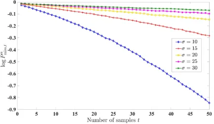
Figure 3 plots the probability of a miss curve (in the logarithmic scale) vs. the number of samples t for five different values of σ, namely σ = 10,15,20,25,30, for the case when the distributions p1 and p2 are uniform, p1 = p2 = [1/3,1/3,1/3]. We observe that for large observation intervals t the curves are close to linear, as predicted by the theory, see Lemma 9. Further, asσincreases the magnitude of the slope decreases becoming very close to0 for large values of σ.

Figure 4 compares the five error exponents curves Sσ(k),

uniform pmfs. As the pmf gradually becomes more and more concentrated, the error exponents monotonically increase, until the highest error exponent curve, corresponding to the most concentrated pmf of the five, with state duration d = 2

occurring most of the time. This result is expected, as it is easiest to detect the process with the lowest entropy, and hence the corresponding error exponent should be the highest.

Figure 4 also plots the theoretical upper and lower bounds in (43) and (34), respectively; we note that, since p1 = p2 in each of the five simulation setups, the same upper bound– equal to 1/2µ2

1/(2σ2) + 1/2µ22/(2σ2)– applies, see eq. (34). The lower bound, equal toµ2

1/(2σ2), is plotted in blue dotted line, while the upper bound is plotted in red dashed line. It can be seen from the figure that each of the five numerical error exponent curves is at all points sandwiched between the lower bound (43) curve µ2

1/(2σ2)and the upper bound curve

1/2µ2

1/(2σ2) + 1/2µ22/(2σ2). Further, the closest curve to the lower bound is the error exponent for the uniform distribution, p1 =p2 = [1/3,1/3,1/3], which is intuitively expected, as also explained in the above paragraph. The curve closest to the upper bound is the most skewed, i.e., sharpest distribution, p1=p2= [0.05, 0.9,0.05].

In order to get further closer to the theoretical error exponent limit, we shift the probability mass from state duration d= 2

to d= 3, and simulate the casep1 =p2 = [0.05,0.05,0.9]. The reasoning is the following: the longer the process stays in the same state, it should be easier to detect it. For complete-ness, we also simulate the case p1 =p2 = [0.9,0.05, 0.05], i.e., when the process often switches from one state to the other. The results, shown in Figure 5, are well aligned with the intuition. The lowest of the three curves is the curve corresponding to the fastest switching process, with most of the mass on the shortest possible duration, d= 1. The highest curve (and the one closest to the theoretical upper bound) is the curve corresponding to the most inert process, when most of the mass is on the longest state duration,d= ∆ = 3, while the curve with the mass concentrated ond= 2is in the middle of the two.

Fig. 3: Simulation setup: ∆ = 3,p1=p2= [1/3,1/3,1/3], µ1= 2,µ2= 5,α= 0.01. Evolution of probability of a miss, in the logarithmic scale, forσ= 10,15,20,25,30.

In the second set of experiments, we consider the setup where the signal level in state 1 is zero,µ1 = 0, and µ2 =

µ= 1; similarly as in the previous setup, we consider uniform

Fig. 4: Simulation setup: ∆ = 3,µ1= 2,µ2 = 5, α= 0.01. σvaries from5 to50. The five middle full lines plot the nu-merical error exponents estimated from slope oflogP_missα _,tvs. σ, for 1) p1 =p2 = [1/3, 1/3,1/3](yellow); 2) p1 =p2 = [0.25,0.5,0.25] (turquoise); 3) p1 = p2 = [0.15, 0.7,0.15] (pink); and 4)p1=p2= [0.1,0.8,0.1](light green); and 5) p1=p2= [0.05,0.9,0.05](brown). Blue dotted line plots the theoretical lower boundµ2

1/(2σ2)in (43) and red dashed line plots the upper bound 1/2µ2

1/(2σ2) + 1/2µ22/(2σ2)in (34)

Fig. 5: Simulation setup: ∆ = 3, µ1 = 2, µ2 = 5, α = 0.01. σ varies from 5 to 50. The three middle full lines plot the numerical error exponents estimated from slope of logPα

miss,t vs. σ, for 1) p1 = p2 = [0.9,0.05,0.05] (brown); 2) p1 = p2 = [0.05,0.9,0.05] (light green); and 3) p1 =p2 = [0.05,0.05,0.9] (pink). Blue dotted line plots the theoretical bound µ2

1/(2σ2) in (43) and red dashed line plots the upper bound 1/2µ2

1/(2σ2) + 1/2µ22/(2σ2)in (34).

distributionsp1, p2∼ U([1,∆]), with∆ = 2. We compare the numerical error exponent with the one obtained as a solution to optimization problem (46). To solve (46), we apply random search over106_{different vectors from setV, and pick the point} which gives the smallest value of the objective (and satisfies the constraint in (46)).

Figure 6) their slopes continuously increase with the increase of the observation interval. As a consequence, the linear fitting performed on the whole observation interval is underestimat-ing the slope, as it is tryunderestimat-ing to fit also the region of values where concavity is more prominent. To further investigate this effect, we performed linear fitting of probability of a miss curves only for a region of higher values oft, where emergence of linearity is already evident. In particular, for each different value of σ, we apply linear fitting for[4/5tmax, tmax], where tmax is the maximal t for which the probability of a miss is non-zero, and we plot the results in Figure 7, bottom. It can be seen from the figure that the numerical curve got closer to the theoretical curve, indicating that the bound in (46) is very tight or even exact. Finally, it can be seen from Figure 7 (top and bottom) that the value of σfor which the error exponent is equal to zero matches the threshold predicted by the theory, σ? _{= µ/(2}√_{2 log ∆) = 0.4247, obtained from detectability}

condition (45).

Fig. 6: Simulation setup: ∆ = 2, p1, p2 ∼ U([1,∆]), µ1 =

0, µ2 = 1, α = 0.01. Plots of probability of a miss in the logarithmic scale forσ= 0.3,0.33,0.37,0.4,0.45

Comparison with the HMM detector. To illustrate the difference between the HSMM and the HMM, we compare the performance of the optimal HSMM detector derived here with HMM-based detector, derived in [22], see Proposition 1. Namely, we run both detectors on the same data generated by an HSMM model, with certain pmfs. In particular, we set

∆ = 5and consider two sets of simulations: 1) truncated geo-metric pmfsp1,g=p2,g= 1/(1−q∆)((1−q), q(1−q), q2(1− q), q3_{(1−q), q}4_(1−q))∈R5_{, whereq= 0.8; and 2)} concen-trated pmfsp1,c=p2,c= (0.025,0.025,0.025,0.025,0.9)∈ R5_{, see paragraph on the comparison with random telegraph} signal in Section II. In the first case we set the HMM transition matrix asPHMM= [q, (1−q); (1−q), q], which ensures that the resulting distribution of the state durations will be close to p1,g = p2,g. Since the data is in this case well fitted by

the HMM, we expect that the non-optimal but tuned HMM-based detector will behave close to the optimal HSMM-HMM-based detector. In the second case, the pmfs cannot be fitted by a geometric distribution, but we keep the same transition matrix PHMM, as it describes well the property that the process stays the same time in both states. Since in this case the data is far from an HMM, we expect that the optimal HSMM-based detector will outperform the HMM-based detector.

Fig. 7: Simulation setup: ∆ = 2, p1, p2 ∼ U([1,∆]), µ1 = 0, µ2 = 1, α = 0.01. σ varies from 0.2 to 0.6. Blue full line plots the numerical error exponent estimated from slope of logPα

miss,t vs. σ by linear fitting. Top: linear

fitting performed on the whole interval [1, tmax]; bottom: linear fitting performed on [4/5tmax, tmax]. Red dashed line plots the theoretical bound calculated by solving (46)).

Fig. 8: Simulation setup: (upper) ∆ = 5, σ = 10, µ1 = 2, µ2 = 5, α = 0.01. Top: p1,g = p2,g = 1/(1−q∆)((1− q), q(1−q), q2_{(1−q), q}3_{(1−q), q}4_{(1−q)), whereq= 0.8;} bottom: p1,c = p2,c = (0.025,0.025, 0.025,0.025,0.9). The curves plot the probability of a miss logPα

miss,t (in the