Optimistic irrationality and overbidding in private value auctions

City, University of London Institutional Repository

Citation

:

This is the accepted version of the paper.

This version of the publication may differ from the final published

version.

Permanent repository link:

Link to published version

:

Copyright and reuse:

City Research Online aims to make research

outputs of City, University of London available to a wider audience.

Copyright and Moral Rights remain with the author(s) and/or copyright

holders. URLs from City Research Online may be freely distributed and

linked to.

City Research Online: http://openaccess.city.ac.uk/ publications@city.ac.uk

Optimistic Irrationality and Overbidding in Private

Value Auctions

Sotiris Georganas

City University London

Social Sciences Building

St John Street, EC1R 0JD, London, UK

Dan Levin

Ohio State University

1945 N. High Street

Columbus, OH 43210, USA

Peter McGee

University of Arkansas

Business Building

Fayetteville, AR 72701, USA∗

December 27, 2016

Abstract

Bidding one’s value in a second-price, private-value auction is a weakly dominant solution (Vickrey, 1961), but repeated experimental studies find

more overbidding than underbidding. We propose a model of optimistically

irrational bidders who understand that there are possible gains and losses associated with higher bids but who may overestimate the additional proba-bility of winning and/or underestimate the potential losses when bidding above value. These bidders may fail to discover the dominant strategy—despite the fact that the dominant strategy only requires rationality from bidders—but re-spond in a common sense way to out-of-equilibrium outcomes. By varying the monetary consequences of losing money in experimental auctions we observe more overbidding when the cost to losing money is low, and less overbidding when the cost is high. Our findings lend themselves to models in which less than fully rational bidders respond systematically to out-of-equilibrium incen-tives, and we find that our model better fits the effects of our manipulations than most of the existing models we consider.

JEL classification: C92, D44, D82

Keywords: auctions, dominant strategy, out of equilibrium payoffs

∗_{Corresponding author, E-mail: pmcgee@walton.uark.edu, Phone:(479)575-4003,}

Fax:(479)575-3421. We are grateful to participants at the ESA Ft. Lauderdale Meetings, the 2009 Econometric Society Meeting, CRETE 2015, and numerous seminar participants for their helpful suggestions,

and especially to John Kagel for his insightful comments. We also thank the editor and two

1

Introduction

In a sealed-bid second-price auction (SPA) with private valuations, where the highest

bidder wins and pays the second highest bid, bidding one’s value is a weakly

dom-inant strategy (WDS, Vickrey 1961). This strategy requires only that each bidder

behave rationally and it is unaffected by the number of rivals or their valuations, a

bidder’s risk preferences, or beliefs regarding rationality of rivals. Repeated

experi-mental studies have found that subjects deviate from the WDS by overbidding much

more than underbidding, resulting in overbidding on average (e.g., Kagel, Harstad

and Levin 1987; Kagel and Levin 1993). By contrast, experimental evidence from

the strategically equivalent ascending English auction demonstrates almost

immedi-ate convergence to the dominant strimmedi-ategy (e.g. Kagel, Harstad, Levin 1987; Kagel

and Levin 1993; Kagel 1995).1 _{While overbidding relative to the risk-neutral, Nash}

equilibrium (RNNE) has also been frequently found in first-price auctions (FPA,

e.g., Kagel 1995 and Kagel and Levin 1993), the “usual suspects,” — risk aversion,

beliefs about others’ play, biases in perceptions of probabilities — that may explain

overbidding in FPAs are of no avail in SPAs.

The contrast between SPAs and English auctions suggests that subjects discover

the WDS in the English auction but not in the SPA; why is this the case? The

cognitive process that leads to the discovery of the WDS in an SPA is far from

trivial and an experimental subject may be unable to recognize it without experience

1_{Given the differences in the strategy spaces, it is not strictly accurate to say that the two}

or training. In an English auction, on the other hand, a subject needs to answer a

simple question for herself: “Am I ‘in’ or ‘out’ ?” Answering this question leads a

bidder to drop out at his value.

Subjects who do not bid their value in SPAs are nevertheless still motivated by

common sense economic incentives, such as expected payoffs, though imperfectly.

Kagel, Harstad, and Levin (1987) conjectured that subjects are aware that higher

bidding increases the probability of winning the auctions but underestimate the

addi-tional cost associated with it. Instead of looking for dominant strategies, we suggest

thatoptimistically irrational bidders are guided by a desire to maximize their profits

combined with an inability to fully grasp the intricacies of the auction environment

that allows them to view the consequences of their actions more favorably. We do this

by modeling reasonable bidders who recognize (i) a higher bid increases the

proba-bility of winning, and (ii) the bidder may understate negative payoffs to higher bids.

These behaviorally plausible assumptions about bidders are the building blocks of

our simple model of how out-of-equilibrium incentives might affect behavior in SPAs.

We test our model in SPAs in which we introduce a parameter that changes

the expected payoff as a function of one’s bid but does not affect the WDS. The

parameter multiplies realized losses by some amountβ, where β = 1 is the standard

case. Consistent with previous results we find that when 0 < β ≤ 1, overbidding is

pervasive. In contrast, when we change β to 20, overbidding is significantly reduced

and underbidding is more prevalent. Overbidding when 0< β ≤1 results in very few

and fairly small losses (5.8% of auctions; median loss of $0.10). This is a product

number of bidders, so the second highest bid is almost always below the highest

value, even with overbidding. This allows us to rule out a “hot stove” type of learning

whereby losses reduce overbidding in subsequent auctions.2 Instead, it appears that

the dramatic reduction in overbidding occurs when β is exogenously and publicly

increased and can be attributed to changes in expected out-of-equilibrium payoffs.

While explanations for overbidding in various auction formats abound, and we

compare the fit of our model to several of them in Section 5, the contribution of our

model lies in its focus on the dominant strategy, adding to the recent theoretical

interest in how dominant strategies influence decision calculus in games (e.g.,

obvi-ous strategy-proofness, Li 2016). Our strong findings suggest that incentives outside

equilibrium affect behavior in predictable ways in the laboratory, and probably in

the field as well, even when equilibrium analysis predicts otherwise. Goeree et al.

(2002) show a similar result in a FPAs, but in FPAs, as in many other games where

Nash equilibrium is the solution concept, best responding requires “cardinal”

com-putations. Since such computations often involve a high degree of complexity and a

heavy mental cost, we do not expect that the outcome in FPAs will exactly reflect

2_{The change in behavior we observe is immediate, once the β parameter changes, and more}

extreme than could be plausibly predicted by learning models, as they would usually be applied (note that little is known about learning transfer between different but very similar games, such as

the ones that result from the manipulation ofβ). In particular, reinforcement learning (Erev and

Roth 1998) would predict no change in behavior before subjects have a chance to experience the new payoffs, unlike what we observe in the data. Fictitious play (Fudenberg and Levine 1998) is also unlikely to fit the data, since the overbidding we observe can not be justified by any beliefs. Other models, such as learning direction theory (Selten and Stoecker 1986) and EWA (Camerer and Ho 1999), consider foregone payoffs. These might predict a faster response in auctions than other models, but its still hard to conceive how they could predict such an immediate change in bidding,

whenβ changes, after the subjects have already been learning for 20 or 40 periods. Steady state

concepts such as QRE (McKelvey and Palfrey 1995) are better suited to the task, e.g. predicting

the immediate tendency towards value bidding whenβ rises without a need for subjects to actually

the point prediction of Nash equilibrium. It is much less surprising to find that the

subjects’ calculations, possibly involving heuristics, approximations and

simplifica-tion rules, will be affected by a change in the incentives, even if these ought to have

no effect on Nash equilibrium. This complexity motivates many models that predict

overbidding by allowing bidders to make, and learn from, mistakes (e.g., QRE). In

an SPA with private values, however, the dominant strategy can be reached with

just “ordinal logic” of dominance, without even a need for common knowledge of

rationality.3 _{Thus, one would expect the solution norm— bid your value —to have}

its best chance for success in this environment. Our study shows that behavior is

still guided by some degree of conscious profit maximization, but subjects’ decision

processes fail to recognize a characteristic that is very seldom present outside the

lab: the dominant strategy. Errors in recognizing a dominant strategy require a

new perspective on the cognitive processes underlying bidding behavior of the sort

provided byoptimistic irrationality to try to explain “errors” made by bidders that

are as much a function of the simplicity of a dominant strategy as the complexity of

the environment.

2

Optimistically Irrational Bidders

The overlooked availability of a WDS must be the starting point of any explanation

to overbidding in SPA. We formalize the intuition behind the conjecture laid out in

3_{Levin, Peck and Ivanov (2016) is devoted to separating failures of “ordinal logic” (or “insight”)}

Kagel, Harstad, and Levin (1987) by modeling an “optimistically irrational” bidder

who understands that there are possible gains and losses associated with higher bids

but who may overstate the additional probability of winning due to higher bidding

and/or understate the losses associated with it.4

Let there benrisk-neutral bidders, each of whom privately observes her valuexi,

i= 1, ..., n. It is common knowledge that thexi’s arei.i.ddraws from a distribution

with a cumulative density function F(t), where F0(t) = f(t) > 0 on [0,1], F(0) =

0, and F(1) = 1. For our purposes, we assume that the xi’s are drawn from a

generalized uniform distribution, F(t) = tbα and

b

α ≥ 1, where α_b = 1 corresponds

to the uniform distribution used in almost all laboratory SPAs and FPAs. We first

make four assumptions:

Assumption 1. Symmetry

Assumption 2. Upon winning, a bidder’s gross payoff is x.

Assumption 3. Bidders believe values are i.i.d from a c.d.f. F(t) = tα _{withα ≥}

b

α.

Assumption 4. A bidder with a valuexwho bidsb > xand wins at a pricep∈(x, b)

believes that the expected payment is γ(x)b+x₂ , with0< γ(x)≤1, i.e., expected losses are x−γ(x)b+x₂ .

The first two assumptions simply mean that each bidder believes that all other

bidders use the same, strictly monotonic bidding function, and that they receive their

4_{The conjecture is as follows, “Bidding in excess ofx in the second-price auctions would have to}

be labeled as a clear mistake, since biddingx is a dominant strategy irrespective of risk attitudes.

Bidding in excess ofx is likely based on the illusion that it improves the probability of winning

full value if they win the auction. Assumption 3 implies that a bidder potentially

overstates the impact of bidding past his value because he believes values are closer

together than they actually are. That is, he believes the increase in the probability

of winning corresponding to an increase in his bid is greater than it actually is. This

assumption finds support in other studies of auctions. For example, Cooper and

Fang (2008) found that subjects who perceive their rivals to have values similar to

their own are more likely to overbid in experimental SPAs, while Breitmoser (2015)

uses “projection,” the tendency to believe that rivals have value or beliefs similar to

one’s own, to explain the winner’s curse.5 _{Finally, Assumption 4 captures the notion}

that a bidder in an SPA may understate possible losses when he bids above his value

and wins.

These assumptions allow us to make two important observations about an

opti-mistically irrational bidder’s maximization problem

Proposition 1. Sincere bidding, i.e., b(x) =x for all x, occurs if and only if for all

x, γ(x) = 1.

Proof. See appendix.

Proposition 1 means that an optimistically irrational bidder may still bid his

value when α = α_b and γ(x) = 1. This does not require that the bidder recognizes

the availability of the WDS. In fact, sincere bidding only requiresγ(x) = 1 but allows

α >α_b.6

5_{Perception of similarity in Cooper and Fang is induced by information provided to subjects}

about their rivals’ values.

Remark. There is a linear solution to the maximization problem with b(x;α, γ, n) =

δ(α, γ, n)x.7

Put more simply, the bid will be a multiple of the value. The exact multiple

will be a function of the number of competitors, how “close” a bidder believes those

competitors’ values are to his value, and the extent to which he understates the losses

from overbidding. In the next section we make use of the fact that there is a linear

solution to the maximization problem to inform our experimental design.

2.1

Experimental Test of the Model

Optimistically irrational bidders need not recognize the WDS but can be influenced

by “out-of-equilibrium” payoffs. Several authors have argued that, in English or

first-price auctions with private values, the exact shape of the expected payoff

func-tions matters (e.g., Harrison 1989; Goeree et al. 2002; Georganas 2011; Georganas

and Nagel 2011).8 Similarly, Noussair, Robin, and Ruffieux (2004) compare value

revelation using the Becker-DeGroot-Marschak (BDM) method and SPAs and find

that the shape of the expected payoff function may influence behavior. They find

that the shape of the expected payoff function in the SPAs means that the

probabil-ity of winning increases faster in overbids than it decreases in underbidding, which

drives bidders who start out below the WDS towards the WDS, while overbidding

is also more costly in the SPA than in the BDM with three or more bidders. Taken

together, these observations about the shape of the expected payoff function seem

7_{The formal derivation can be found in the appendix.}

8_{Our model of optimistically irrational bidders also predicts bidding above the risk-neutral Nash}

to reflect the assumptions we make in our model. As a simple test of optimistically

irrational bidders, we implement standard second-price, sealed-bid auctions for one

unit of an indivisible good in the laboratory. The WDS predicts that players bid

their values in equilibrium. We introduce a factor β by which we multiply eventual

negative profits of the bidders. β does not affect the equilibrium if bidders are

bid-ding sincerely because no bidder earns negative profits in equilibrium. However, the

bidders’ expected payoff functions do change, given that their opponents follow the

equilibrium strategies; in Figure 1 we plot, for different values of β, the expected

payoff function for a bidder whose rivals bid their values.

Given the remark in the previous section, we can determine how our experimental

treatments will affect the bidding of optimistically irrational bidders. Applying the

theory to our experimental treatments, when a bidder wins with b > x and loses,

his expected payment is β[x−γβb+x₂ ]. A standard SPA corresponds to the situation

where β = 1, such that the expected losses are 1×[x−γ1b+x₂ ]. This allows us to

define γβ as a function of γ in a standard auction, i.e., γ1, which we do by setting

[x−γ1b+x₂ ] =β[x−γβb+x₂ ], and solving forγβ. Doing this, we get

γβ =

β−1

β

2x

b+x + γ1

β (1)

We can substitute b(x) =δx into equation (1) to obtain

γβ =

1

β[

2(β−1)

Plugging equation (2) into the linear solution, we solve the problem numerically.9

The results can be found in Table 1. Assumingα= 1.1 andγ1 = 0.95, i.e., a bidder

slightly overstates the increase in his probability of winning associated with a higher

bid and slightly understates his expected loss, the model predicts that δ∗ increases

monotonically in β and bidding above value that ranges from 9.7% above value for

a β = 0.1 to 0.5% above value for a β = 20. These numerical estimates yield three

testable hypotheses:

Hypothesis 1. Subjects will overbid on average

Hypothesis 2. Subjects will overbid by more on average when β < 1 than when

β = 1

Hypothesis 3. Subjects will overbid by less on average when β >1than when β = 1

3

Experimental Details

The data come from nine experimental sessions conducted at Ohio State

Univer-sity. Students were recruited via e-mail and sessions took place in the Experimental

Economics Lab. The experiment was programmed and conducted with the software

z-Tree (Fischbacher 2007). In every session, subjects participated in 62

second-price, sealed-bid auctions—2 trial auctions followed by 60 paying auctions—with

either three or six bidders per auction. Subjects were randomly and anonymously

re-matched between auction periods.10 _{At the beginning of each auction, subjects}

privately observed their own independent private values denominated in an

exper-imental currency unit (ECU), but they did not observe the values of others. All

values were drawn from a uniform distribution on the interval [0, 100], which was

common knowledge. At the end of each period the bidder who obtained the item

was informed of the price and his profit, while bidders who did not obtain the item

received no information about the price or the bids of others. The instructions can

be found in the appendix.

We multiplied negative profits by a parameter, β, which took on three values in

every session: 1, 0.1, and 20. Beta took on one of these values for periods 1-19,

another for periods 20-39, and the final value for periods 40-60. Subjects knew the

value of β, that it is the same for all bidders, and that they would be made aware

when it changed; subjects did not know when β would change, how many times it

would change, or what its magnitude would be. All subjects were given starting

balances of 150 ECUs to cover the possibility of losses. Profits and losses were added

to this balance and the balance was paid at the end of each session. We ran two

sessions with 3 bidder auctions and a β order of 1, 0.1, 20 (β_1/0.1/203 ), two sessions

with 6 bidder auctions and a β order of 1, 0.1, 20 (β_1/0.1/206 ), two sessions with 3

bidder auctions and a β order of 1, 20, 0.1 (β3

1/20/0.1), and three sessions with 3

bidder auctions and a β order of 20, 1, 0.1 (β3

20/1/0.1). In sessions with three bidder

auctions, the exchange rate was $1=20 ECU, while the exchange rate in sessions

with six bidder auctions was $1=14 ECU. The exchange rates were different in order

to equalize the expected payoff between sessions with different group sizes. In the

event that a player went bankrupt, they were no longer permitted to bid and were

paid a participation fee of $8. Due to the uneven numbers after a bankruptcy, at the

beginning of every period after a bankruptcy two subjects were randomly assigned

to sit out that period in 3 bidder auctions, while five subjects were chosen to sit

out in 6 bidder auctions. In the six sessions that started with β = 1, there were

two bankruptcies; in the three sessions that started with β = 20 there were 10

bankruptcies, with all but one occurring in the first 10 periods. Complete session

details can be found in Table 2.

4

Results

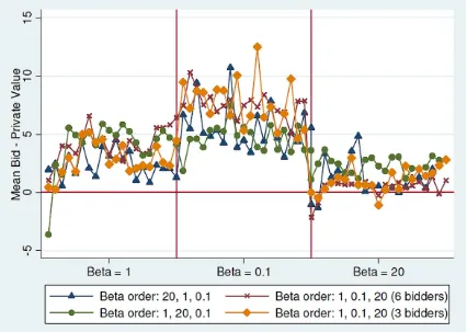
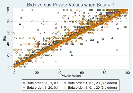
Average differences between values and bids can be found in Table 3, and Figures

2-6 compare subjects’ bids and their values. Consistent previous research, we see

overbidding on average in every treatment for every value of β. To test whether or

not this overbidding is significantly different from 0, we calculated the mean difference

between bid and private value for each session within a β regime, i.e., the block of

periods during which β remained the same. Using these means as our measure of

overbidding, average overbidding is significantly greater than 0 at the 5% level in

every case except for β = 20 for β3

1/0.1/20 (t-test p = 0.174) and β1/0.1/206 (t-test

p= 0.129).

values of β.

The effects of changes in β are visible and drastic, in contrast to the standard

theoretical prediction of no change at all. For example, when we reduce the

punish-ment for negative outcomes from β = 1 to β = 0.1 in period 20 of β3

1/0.1/20, there

is an immediate effect as the average difference between bid and value more than

doubles from approximately 2.8 to 7.5— an increase equal to approximately 5% of

the support of values. When β rises to 20 in period 40 and punishment for negative

outcomes is severe, the overbidding largely disappears, with average overbids falling

from 7.5 to 1.1. Similar patterns emerge in all treatments, and the differences in

overbidding across β regimes are significant.11,12

Observation 2. Consistent with Hypotheses 2 and 3, overbidding varies significantly

across different values of β, with higher levels of β leading to less overbidding.

Our specific design allows for an additional important and interesting observation

about learning. There is significant overbidding in the first 40 periods with β = 1

andβ = 0.1 inβ3

1/0.1/20 andβ 6

1/0.1/20 , and we do not observe learning in the direction

of value bidding in these periods.13 _{Nonetheless, there is a drastic reduction of}

11_{To compare overbidding, we conducted Wilcoxon signed rank tests on the session means we}

calculated for the various β regimes. In pairwise tests of each value of β for all treatments, all

differences were significant at the 5% level or better except forβ = 1 versusβ= 0.1 forβ3

1/20/0.1(p=

0.454).

12_{Merlob, Plott, and Zhang (2012) compare auction designs used for Medicare and Medicaid}

procurement auctions. In auction designs that allow for costless reneging, which is similar to

bidding in an auction withβ <1, they also find overbidding.

13_{We divide those periods for whichβ= 0.1 in these treatments, i.e., periods 20-39, into 4 blocks}

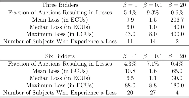
overbidding in period 40. One possible explanation for the decline in overbidding in

period 40 is that subjects who have overbid in earlier periods are chastened by losing

money, a sort of “hot stove” learning. The evidence in Table 4 does not support this

explanation. Before β increases to 20, few auctions result in realized losses. They

range from a minimum of 4.3% of auctions for the case with six bidders whenβ = 1,

to 9.3% with three bidders andβ = 0.1. The average loss is also quite small, ranging

from 1.1 ECUs with six bidders and β = 0.1, to 10.8 ECUs with six bidders and

β = 1. Moreover, this small and infrequent negative feedback for the first two levels

ofβ appears to have no effect on those who experience it. Of the 31 bidders who lose

money when β = 1, 29 also lose money when β = 0.1. Of the six bidders who lost

money when β = 20, 5 lost money at all three levels of β and the sixth lost money

when β= 0.1.

Observation 3. Reductions in overbidding when β is increased are not caused by

learning due to previous losses.

In order to move beyond unconditional means and investigate the effects of β

while allowing for individual heterogeneity, we estimate a random effects Tobit model,

regressing the difference between subjecti’s bid and his value in auctionjon dummies

for each β regime.14

The results in columns 1-4 of Table 5 are similar to the means in Table 3. In every

treatment bids are significantly higher when β = 0.1 than when β = 1; similarly,

bidding is significantly lower in every treatment when β= 20 than when β = 1. We

do, however, see some differences across treatments, and we reject the null hypothesis

14_{In the experiment, subjects could not bid more than 100, which can be seen in the groups of}

that the marginal effects of Dβ=0.1 and Dβ=20 are jointly equal across all treatments

(Wald test,p= 0.000 for both).

Although learning due to negative reinforcement is unlikely inβ_1/0.1/203 andβ_1/0.1/206 ,

one possible explanation for the differences across treatments we observe may be

some other sort of learning or experience. To address this possibility, we augment

the model in columns 5-8 with a linear time trend and its interaction with the β

regime. We observe small, but statistically significant increases in bids over time in

the first 20 periods in treatmentsβ6

1/0.1/20,β 3

1/20/0.1, and β 3

20/1/0.1, where bids increase

by roughly 0.12 to 0.18 ECUs per period; we see no significant changes over time in

subsequent periods. With the inclusion of the time trend, the same pattern emerges:

greater overbidding when β = 0.1 and less overbidding when β = 20, though the

treatment effects are no longer significant in β_1/20/0.13 . Allowing for changes to

bid-ding behavior over time, we cannot reject the null hypothesis that the marginal

effects ofDβ=0.1 and Dβ=20are the same across all treatments (Wald tests, p= 0.551

and p= 0.318, respectively); we find no significant differences at conventional levels

across treatments in pair-wise comparisons ofDβ=0.1 and Dβ=20.15,16

Observation 4. The effects of changes in β are robust to controls for individual

differences and learning over time.

15_{The only pairwise comparisons with p-values less than 0.2 are comparisons of Dβ}

=20 in

β3

1/20/0.1with all other treatments.

16_{One possible motivation for overbidding not found in Table 4 is spite. Cooper and Fang (2008)}

The linear trend presupposes that the effect of all periods is the same within a

β regime, however Figure 2 suggests that the first few periods in a session might be

slightly different.17 In columns 9-12 we estimate the same model as in columns 5-8

but exclude the first 3 periods in each session. After excluding the first three periods,

there is no significant learning over time for any value ofβ in any treatment.

Observation 5. Bidding behavior evolves substantially in the first few periods of a

session, but little thereafter.

5

Alternative models

One important test of our model of optimistically irrational bidders is how well it

fits the data relative to existing models. Among our candidate models, we begin by

considering a symmetric Nash equilibrium (SNE) with normally distributed errors,

given that without errors the SNE fails completely to predict the change in bidding

when we shiftβ. Models that take all payoffs into account, even if they are not on the

equilibrium path, are good candidates to explain our results. Perhaps the simplest

way to consider all payoffs is to use the Nash model but assume that subjects’ errors

depend on the expected utility of each action in a systematic way. We do this by

considering an SNE with a logistic error structure, as in Crawford and Iriberri (2007).

Finally, we consider is quantal response equilibrium (QRE), which also makes explicit

use of the payoff function shapes, by positing that players choose an action with a

17_{All sessions began with either β = 1 or β = 20, so the relevant data are the first few data}

probability proportional to its expected payoff.18 _{In preliminary comparisons, we}

find that the SNE+normal model outperforms the other two models in all but one

β-number of bidder combinations.19 The reason is that, under a logit error structure,

a high frequency of underbidding is predicted for intermediate private values, since

the expected payoffs are quite flat to the left of the maximum (as seen in Figure 1);

yet we see far more overbidding than underbidding in all cases.20 _{QRE improves on}

the Nash model with logistic errors, but still performs worse than the Nash model

with normal errors.

One way to account for the fact that we observe much more overbidding than

underbidding is to allow bidders to experience joy-of-winning (JOW). JOW can be

incorporated by adding an extra fixed utility, Ui, to the payoff of subject i,

condi-tional on winning the auction.21 It is easy to show that with such modification a

18_{Another possible model that we do not consider is a level-k model of the sort used to explain}

auction results in Crawford and Iriberri (2007). This model predicts neither overbidding nor reaction

to different values of β, even allowing symmetric errors. In such a model, players of level one or

higher are characterized by different beliefs, but they all best respond to these beliefs. Since bidding one’s value is a weakly dominant strategy in a SPA and does not depend on a player’s beliefs (or risk attitudes), players of all levels are predicted to bid their values, as in any Nash equilibrium.

19_{Table A1 in the appendix provides the details of the comparison of fits among all alternative}

models we consider.

20_{For example, for a value of 50 andβ = 0.1 we should see approximately the same amount of}

underbidding as overbidding, which is clearly not the case.

21_{Note that JOW looks superficially similar to spiteful behavior (e.g., Andreoni et al. 2007,}

Cooper and Fang 2008). The difference is that a subject experiences JOW only in the case where she wins, while a subject exhibits spite even if she does not win but in cases where she raises the price for other bidders. In Cooper and Fang’s experiment, for example, subjects can sometimes acquire information about their rival’s value. They find that, when subjects know that their value is close to their rival’s, overbidding is more likely to result in a costly loss and subjects overbid by less. Conversely, when subjects know that their value is well below their rival’s, hence overbidding is unlikely to result in winning the auction but can raise the price for their rival, overbids are larger.

This is not dissimilar to our manipulation ofβ, and Cooper and Fang suggest that this behavior

new dominant solution emerges, with bi(xi) = U_βi +xi.22 This implication helps as

it predicts that players who enjoy winning will overbid with respect to the Nash

equilibrium and the amount of overbidding will depend inversely on β. The JOW

parameter j is found to be positive and yields a significantly higher likelihood in

every case. Nonetheless, SNE with normal errors still provides the best fit among

JOW models.

To evaluate its broad applicability, in Table 6 we examine how well the SNE

models with normal errors, both with and without JOW, fare against our model

of optimistically irrational (MI) bidders in SPAs, English auctions, and FPAs, by

comparing estimated log-likelihoods.23,24 We find that our model fares better than

the SNE with just normal errors (but no JOW) in all auctions. On the other hand, the

SNE with normal errors and JOW outperforms our model in every auction. The SNE

with normal errors and JOW may have slight advantages by the measure of Table 6,

but these advantages do not reveal the full story. In Table 7 we break out the fit by the

number of bidders and values ofβ. In this case, the SNE fares better than MI in six of

the nineβ-number of bidder combinations. In Table 8, we compare the the predicted

mean overbidding by optimistically irrational bidders and the SNE with JOW to the

observed mean overbidding. In 4 out of the 7 cases, the magnitude of overbids by MI

22_{Details are provided in the appendix.}

23_{The English auction data come from Georganas (2011), and the FPA data come from Dyer et}

al. (1989).

24_{The derivation of optimistic irrationality for FPAs can be found in the appendix. The}

bidders is closer to the predicted overbidding than SNE bidders who experience JOW.

While on a strictly econometric basis, SNE+JOW seems to be performing slightly

better than MI, MI outperforms SNE+JOW in several instances.25 Moreover, there

are good qualitative reasons not to be satisfied with JOW, chief among them its

failure to explain why JOW occurs in SPAs but not in the strategically analogous

English auction. Ultimately, further work and additional data will be needed to

completely analyze the relative strengths of the two models.

6

Conclusions

Experiments consistently find that in second-price, sealed-bid auctions with private

values— a mechanism with incomplete information where bidding one’s value is a

WDS — subjects deviate significantly from the WDS. The availability of a

“domi-nant” action that is best irrespective of the other features of the decision is rare in

games with incomplete information and in strategic situations outside the lab. The

behavior of a bidder in a second-price auction who fails to recognize or discover such

an available strategy is still likely to be guided by rules that are useful in a wide range

of situations, such as cost-benefit analysis. Subjects in our SPAs provide support

for this characterization of bidders: their bidding is reasonable if not optimal.

Sub-jects overbid on average but their overbidding is influenced by manipulations which

affect expected payoffs out of equilibrium but not the dominant strategy. In

accor-dance with lessons learned in more familiar settings, as we vary the magnitude of

25_{Although we do not include the SNE model with normal errors and JOW in Tables 7 and 8,}

the penalty for losses, a natural reaction is to hedge and bid lower when the penalty

is relatively larger and to be more aggressive when the penalty is relatively lower.

The behavioral changes may not be optimal in a second-price auction, yet they are

sensible when viewed through the lens of their applicability in richer environments.

We propose a model of optimistically irrational bidders who fail to recognize the

availability of a dominant strategy. Bidders in this model understand that raising

their bid increases the probability of winning but may either overstate the increase in

the likelihood of winning and/or fail to appreciate the costs associated with increasing

their bids. We fit several existing models designed to explain overbidding using our

data, but we find that most of these models perform poorly even when they consider

out-of-equilibrium payoffs that would be affected by our experimental manipulation,

and none of the models outperform ours consistently.

Our results build on the cautiously optimistic findings in Cooper and Fang (2008).

They find that bounded rationality—more than non-standard preferences like spite

and JOW—contributes to overbidding in SPAs. Subjects in their experiment could

purchase costly and noisy information about rivals’ values, information which does

not affect the WDS. Subjects who purchase the information were significantly more

likely to overbid, but the behavior of those subjects who did not purchase

informa-tion was consistent with theoretical predicinforma-tions. They conclude by noting that this

heterogeneity may be of less significance outside the lab where selection might weed

out the irrational bidders, leaving only rational bidders. Our finding of large and

the-oretically unpredicted responses to our treatments can inform mechanism designers,

insuffi-cient or too slow: even in cases with a dominant strategy, the nature of incentives

outside equilibrium can influence behavior. In instances where the common sense

implications of manipulating out-of-equilibrium incentives can steer behavior toward

the desired norm, such as in SPAs, designers may be able to use these incentives to

design more stable and efficient mechanisms.26

26_{While our results are most applicable to situations with a dominant strategy, the fundamental}

Figure 1: Expected payoff functions in a second price auction with 3 bidders, for the three

different values of β. There are 5 curves in every panel which represent expected utility,

Table 1: Numerical estimates of parameters for optimistically irrational bidders in auctions with 3 bidders

β

0.10 0.20 0.50 1 2 10 20

δ 1.0965 1.0889 1.0715 1.053 1.0352 1.0093 1.0048

γβ 0.9141 0.9202 0.9345 0.9500 0.9664 0.9909 0.9952

Note: The numerical solution was found using fzero in Matlab, assuming α= 1.1

and γ1 = 0.95. The highlighted values of β correspond to the values used in the

experiment.

Table 2: Summary of sessions

Treatment Sessions Bidders Ex. Rate Subjects β order Subject-Auctions

β3

1/0.1/20 2 3 14 24 1, 0.1, 20 1398

β6

1/0.1/20 2 6 20 42 1, 0.1, 20 2519

β3

1/20/0.1 2 3 14 33 1, 20, 0.1 1898

β3

Table 3: Mean difference between bid and value by treatment

β = 1 β = 0.1 β = 20 Bidders β order

2.79 7.46 1.07 3 1, 0.1, 20

(6.75) (13.67) (5.61)

4.07 7.54 0.43 6 1, 0.1, 20

(10.26) (12.96) (4.60)

4.04 4.62 2.32 3 1, 20, 0.1

(10.64) (9.94) (5.72)

2.37 5.64 1.13 3 20, 1, 0.1

(7.04) (10.61) (9.08)

Note: Standard deviations in parentheses.

Table 4: Subjects experiencing losses withβ order 1, 0.1, 20

Three Bidders β = 1 β = 0.1 β = 20

Fraction of Auctions Resulting in Losses 5.4% 9.3% 0.6%

Mean Loss (in ECUs) 9.9 1.5 206.7

Median Loss (in ECUs) 6.0 1.0 140.0

Maximum Loss (in ECUs) 43.0 8.0 400.0

Number of Subjects Who Experience a Loss 11 14 2

Six Bidders β = 1 β = 0.1 β = 20

Fraction of Auctions Resulting in Losses 4.3% 7.1% 0.4%

Mean Loss (in ECUs) 10.8 1.6 65.0

Median Loss (in ECUs) 6.5 1.1 30.0

Maximum Loss (in ECUs) 88.0 8.8 180.0

T able 5: Estimated co efficien ts from a random effects T obit mo del of the effec t of β on bids Dep e nd e n t V ariable: Bid-V alue T reatmen t β

3 1/

0 . 1 / 20 β

6 1/

0 . 1 / 20 β

3 1/

20 / 0 . 1 β 3 20 / 1 / 0 . 1 β

3 1/

0 . 1 / 20 β

6 1/

0 . 1 / 20 β

3 1/

20 / 0 . 1 β 3 20 / 1 / 0 . 1 β

3 1/

0 . 1 / 20 β

6 1/

0 . 1 / 20 β

3 1/

References

[1] Andreoni, James; Yeon-Koo Che & Jinwoo Kim (2007) ”Asymmetric

Informa-tion about Rivals’ Types in Standard AucInforma-tions: An Experiment,” Games and

Economic Behavior, vol. 59(2), 240-259.

[2] Breitmoser, Yves (2015) ”Knowing Me, Imagining You: Projection and

Over-bidding in Auctions”, working paper.

[3] Camerer, Colin F. & Teck Hua Ho (1999) ”Experience-Weighted Attraction

Learning in Normal-form Games,”Econometrica, vol. 67, 827-874.

[4] Cooper, David J. & Hanming Fang (2008) ”Understanding Overbidding in

Sec-ond Price Auctions: An Experimental Study,”Economic Journal, vol. 118(532),

1572-1595.

[5] Crawford, Vincent P. & Nagore Iriberri (2007) ”Level-k Auctions: Can a

Non-Equilibrium Model of Strategic Thinking Explain the Winner’s Curse and

Over-bidding in Private-Value Auctions?,”Econometrica, vol. 75(6), 1721-1770.

[6] Dechenaux, Emmanuel; Dan Kovenock & Roman Sheremeta (2015) ”A

sur-vey of experimental research on contests, all-pay auctions and tournaments,”

Experimental Economics, 18(4), 609-669.

[7] Dyer, Douglas; John Kagel & Dan Levin (1989) ”Resolving Uncertainty About

Numbers of Bidders in Independent Private Value Auctions: An Experimental

[8] Fishbacher, Urs (2007) ” z-Tree: Zurich Toolbox for Ready-made Economic

Experiments, Experimental Economics”, Experimental Economics, vol. 10(2),

171-178.

[9] Fudenberg, Drew & David Levine,The Theory of Learning in Games, 1st_edition,

MIT Press, Cambridge, MA, 1998.

[10] Georganas, Sotiris (2011) ”English Auctions with Resale: An Experimental

Study”, Games and Economic Behavior, vol. 73(1), 147-166.

[11] Georganas, Sotiris & Rosemarie Nagel (2011) ”English Auctions with Toeholds:

An Experimental Study,” International Journal of Industrial Organization, vol.

29(1), 34-45.

[12] Goeree, Jacob K.; Charles A. Holt & Thomas R. Palfrey (2002). ”Quantal

Re-sponse Equilibrium and Overbidding in Private-Value Auctions,” Journal of

Economic Theory, vol. 104(1), 247-272.

[13] Harrison, Glenn (1989) ”Theory and Misbehavior of First-Price Auctions”,

American Economic Review, vol. 79(4), 749-762

[14] Kagel, John H. (1995) Auctions: A Survey of Experimental Results In: Kagel,

John H. and Alvin Roth (eds.) The Handbook of Experimental Economics,

Princeton University Press, Princeton NJ

[15] Kagel, John H & Dan Levin (1993) ”Independent Private Value Auctions:

Bid-der Behaviour in First-, Second- and Third-Price Auctions with Varying

[16] Kagel, John H. ; Ronald M. Harstad & Dan Levin (1987) ”Information Impact

and Allocation Rules in Auctions with Affiliated Private Values: A Laboratory

Study”, Econometrica, vol. 55(6), 1275-1304

[17] Levin, Dan; James Peck & Asen Ivanov (2016) ”Separating Bayesian Updating

from Non-probabilistic Reasoning: An Experimental Investigation,” American

Economic Journal: Microeconomics, vol. 8(2), 39-60

[18] Li, Shengwu (2016) ”Obviously Strategy-Proof Mechanisms,” SSRN Working

Paper 2560028

[19] McKelvey, Richard & Thomas R. Palfrey (1995) ”Quantal Response Equilibria

in Normal Form Games,” Games and Economic Behavior, vol. 10(1), 6-38.

[20] Merlob, Brian ; Charles Plott & Yuanjun Zhang (2012) ”The CMS Auction:

Experimental Studies of a Median-Bid Procurement Auction with Non-Binding

Bids”,The Quarterly Journal of Economics, vol. 127(2), 793-828.

[21] Noussair, Charles ; Stephane Robin & Bernard Ruffieux (2004) ”Revealing

Con-sumers’ Willingness-to-Pay: A Comparison of the BDM Mechanism and the

Vickrey Auction,” Journal of Economic Psychology, vol. 25(6), 725-741.

[22] Ockenfels, Axel & Reinhard Selten (2005) ”Impulse balance equilibrium and

feedback in first price auctions,” Games and Economic Behavior, vol. 51 (1),

[23] Roth, Alvin E. & Ido Erev (1998) ”Predicting How People Play Games:

Rein-forcement Learning in Experimental Games with Unique Mixed-strategy

Equi-libria,”American Economic Review, vol. 88, 848-881.

[24] Selten, Reinhart & Rolf Stoecker (1986) ”End Behavior in Sequences of Finite

Prisoner’s Dilemma Supergames: A Learning Theory Approach,” Journal of

Economic Behavior and Organization, vol. 7, 47-70.

[25] Vickrey, William (1961) ”Counterspeculation and Competitive Sealed Tenders,”

Journal of Finance. Vol. 16(1), 8-37.

A

Appendix

A.1

Second Price Auctions

The maximization problem of an optimistically irrational bidder in an SPA in our

model is:

max

b≥0 [σ(b)]

α(n−1)_{x−[[σ(x)]α(n−1)

[σ(b)]α(n−1)]θn(x) + [

[σ(b)]α(n−1)_−[σ(x)]α(n−1)

[σ(b)]α(n−1) ]γ(x)

b+x 2 ]},

where θn(x) denotes the expected price if a bidder wins at a price below his value

and σ(b) denotes the inverse bidding function.

The first-order condition (FOC) for the maximization problem is:

2xα(n−1)[σ(b)]α(n−1)−1σ0(b)−γ(x)α(n−1)[σ(b)]α(n−1)−1σ0(b)(b+x)

After simplifying we have:

2xα(n−1)[σ(b)]α(n−1)−1[1−γ(x)]σ0(b)−γ(x)α(n−1)[σ(b)]α(n−1)−1(b−x)σ0(b)

−γ(x)[[σ(b)]α(n−1)−[σ(x)]α(n−1)] = 0

(A.1)

Proof of Proposition 1

Proof. Assume that ∀x∈[0,1], b(x) =x. In such a case equation (A.1) becomes

2xα(n−1)[σ(b)]α(n−1)−1(1−γ(x)) = 0

implying γ(x) = 1, for all x >0, asσ0(b) = 1 with b(x) :=x.

Assume that ∀x∈[0,1],γ(x) := 1. In such a case equation (A.1) becomes

−{[α(n−1)σ(b)]α(n−1)−1(b−x)σ0(b)+[[σ(b)]α(n−1)−[σ(x)]α(n−1)]}_Q0 as b(x)_Tx.

Derivation of remark 1

Consider the FOC in equation (A.1). Recognizing that at the solution σ(b) =x

and σ0(b) = _b01_(x), and simplifying, we can rewrite (A.1) as

2α(n−1)[1−γ(x)]−γ(x)α(n−1)(b

x −1)−γ(x)b 0

(x)[1−(σ(x)

x )

α(n−1)

Assume that ∀x ∈ [0,1], γ(x) = γ < 1 and b(x) = δx, with δ ≥ 1. Equation (A.2) can be written as:

2α(n−1)[1−γ]−γα(n−1)(δ−1)−γδ[1−(1

δ)

α(n−1)

] = 0 (A.3)

When δ = 1 then (A.3) becomes 2α(n−1)[1−γ]> 0 when γ < 1, which is the

case for overbidding.

By inspecting (A.3), it is clear that the LHS is strictly declining in δ, so that

there is a unique δ∗ that solves

2α(n−1)[1−γ]−γα(n−1)(δ∗−1)−γδ∗[1−(1

δ∗)

α(n−1)

] = 0 (A.4)

A.2

First Price Auctions

The maximization problem of an optimistically irrational bidder in an FPA:

max

B≥0[σ(B)]

α(n−1)_{[x−B] (A.5)}

Denote the solution to (??) by B(x;α) and the risk-neutral Nash equilibrium by

B(x;α_b).It is well known that the solution to (5) is given by,

B(x;α) = x−

Rx

0 t

α(n−1)_dt

xα(n−1) =x−

x α(n−1)+1 =

α(n−1) α(n−1)+1x

Proposition 2. B(x;α)≥B(x;α_b) as α≥α._b

Thus, optimistically irrational bidders will bid above the RNNE but below their

value.

A.3

Joy of Winning

Lemma 3. In a second price auction where negative payoffs are multiplied times β

and bidders have a heterogeneous joy of winningUi, the dominant strategy equilibrium

is bi(xi) = U_βi +xi.

Proof. Expected profits in the auctions are Πi = prob{bi > max(b−i)}(xi +Ui −

E[max(b−i)|bi > max(b−i)]), and subjects choose a bi(xi) to maximize Πi. Consider

bidding b0 < bi(xi) = U_βi +xi, when it matters i.e. you win with bi(xi) but lose

with b0. It also means that the price the winner pays is p ∈ [b0, bi(xi)]. If p > xi,

winning earns Ui −β(p−xi) ≥ Ui −β((U_βi +xi)−xi) = 0. When p ≤ xi, strict

positive payoffs are assured. With a similar step we show that biddingbi(xi),weakly

dominates biddingb0 > bi(xi).

A.4

Examining the consistency of joy of winning

The fit of the SNE and the behavioral models is improved when we allow for joy of

winning. But is joy of winning a consistent explanation across all different values of

β that we have used in the experiments? As we have seen, joy of winning gives a

clear prediction for every β. A person who understands the dominant strategy but

has joy of winning j, will overbid by exactly j when β = 1 but will overbid by 10j

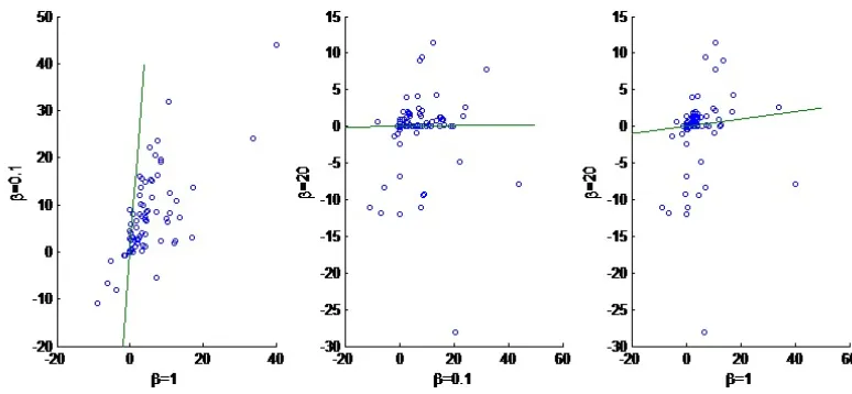
following Figure 6 we examine if individual players’ behavior is consistent with this

model.27

Figure 6: Consistency of the joy of winning hypothesis for each individual across the three

values ofβ.

Every dot is a single observation, plotting the average overbidding of a player for

two different values of β. In the left panel for example, we have mean overbidding

whenβ = 1 in the x axis and mean overbidding whenβ = 0.1 in the y axis. According

to the theory all observations should lie on a straight line through the origin with

slope βx/βy. What we see is that many observations lie on or close to the line.

However there are still some observations, especially in the second and third panel

that lie far away from this line. This indicates that although heterogeneous joy of

winning could at first sight partly explain overbidding in second price auctions, it is

not a fully consistent explanation.

27_{The bidding results of the 3 bidder and 6 bidder case are pooled, as the number of bidders}