Modeling of the onset, propagation and interaction of multiple cracks generated from corrosion pits by using peridynamics

Modeling of the Onset, Propagation and Interaction of Multiple

Cracks Generated from Corrosion Pits by Using Peridynamics

Dennj De Meo1, Luigi Russo1, Erkan Oterkus1, *

1 _{Department of Naval Architecture, Ocean and Marine Engineering, University of} Strathclyde, Glasgow, Lanarkshire, G4 0LZ, UK

Abstract: High stress regions around corrosion pits can lead to crack nucleation and propagation. In fact, in many engineering applications, corrosion pits act as precursor to cracking, but prediction of structural damage has been hindered by lack of understanding of the process by which a crack develops from a pit and limitations in visualisation and measurement techniques. An experimental approach able to accurately quantify the stress and strain field around corrosion pits is still lacking. In this regard, numerical modeling can be helpful. Several numerical models, usually based on FEM, are available for predicting the evolution of long cracks. However, the methodology for dealing with the nucleation of damage is less well developed, and, often, numerical instabilities arise during the simulation of crack propagation. Moreover, the popular assumption that the crack has the same depth as the pit at the point of transition and by implication initiates at the pit base, has no intrinsic foundation. A numerical approach is required to model nucleation and propagation of cracks without being affected by any numerical instability, and without assuming crack initiation from the base of the pit. This is achieved in the present study, where PD theory is used in order to overcome the major shortcomings of the currently available numerical approaches. Pit-to-crack transition phenomenon is modeled, and non-conventional and more effective numerical frameworks that can be helpful in failure analysis and in the design of new fracture-resistant and corrosion-resistant materials are presented.

1. Introduction

accurately and, due to numerical convergence issues, crack branching could not be captured. In the study described in Pidaparti & Rao (2008) [14], a coupled experimental and computer-aided-design (CAD) procedure is used to generate 3D models representing the time evolution of corrosion pits in aluminium alloys. FEM is then used to predict the stress field around pits subjected to static tensile load and the sites of possible crack nucleation. A similar study is reported in [12], where the level of stresses increases and then reaches a plateau with increasing corrosion time. Another model based on FEM is described in Turnbull et al. (2010) [22], where a single pit in a cylindrical steel specimen subjected to tensile axial stress is analysed. The model predicts that, for low applied stress and assuming fully elastic material, the maximum stresses occur at the pit shoulder just below the pit mouth. More complex loading conditions were considered in Rajabipour & Melchers (2013) [15], where corroded pipes subjected to both internal pressure and axial load were considered. The study reported in (Zhu et al. 2013) [24], where FEM was used to predict stress and strain fields around corrosion pits in austenitic stainless steel subjected to ultra-low elastic stress, confirmed that the highest stresses and strains occurred at the pit shoulder and that their magnitudes increases as the size of the pit increases.

2. Pit-to-crack transition

Pitting is a localised form of corrosion that lead to the formation of corrosion cavities or pits due to the breakage of the material’s passive film. Therefore, pitting typically occurs in materials such as stainless steel, aluminium, titanium, copper, magnesium and nickel alloys. Due to material inhomogeneities, pits can evolve in very different shapes as shown in Fig. 1:

Fig. 1 Possible pit morphologies [25]

3. Peridynamics

Peridynamics (PD) is a new continuum mechanics formulation that was presented for the first time to the scientific community in Silling (2000) [16]. PD is a generalisation of CCM, which was introduced by the French mathematician Cauchy more than two centuries ago. The governing equations of CCM are based on partial differential equations (PDEs) and its mathematical formulation breaks down in the presence of discontinuities such as cracks. This limitation can be overcome overcome by peridynamics, whose governing equations are integro-differential, and do not contain any spatial derivatives.

The PD equation of motion (EOM) of a generic material point x can be written as [16]

( ) ( )

(

( ) ( )

)

( )

H

t t t V t

ρ =

∫

x x

x u x f u x u x x x b x ₍₁₎

where u x

( )

( ) ( )

(

)

f u x u x x x represents the PD force between material points x and

′

Fig. 2 PD interactions in 2D

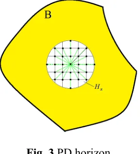
It is assumed that the strength of interaction between material points decreases as the distance between them increases. Therefore, an influence domain, named horizon,H_x, is defined for each material point as shown in Fig. 3.

Fig. 3 PD horizon

the model is able to fairly represent the physical mechanisms of interest [1]. As δ decreases, the interactions become more local and, therefore, Classical Continuum Mechanics (CCM) can be considered as a special case of PD theory.

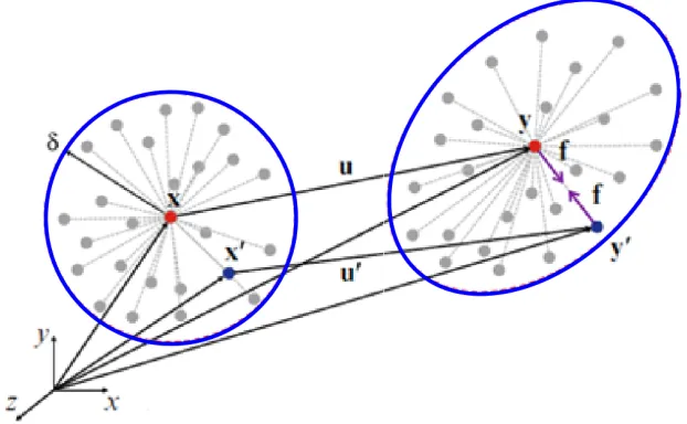
In the case of an elastic material, the peridynamic force between material points x and x′, can be expressed as:

c s ′ − =

′ − y y f

y y (2)

where y represents the location of the material point x in the deformed configuration as shown in Fig. 4, i.e. y x u= + , while c is the bond constant which can be related to material constants of CCM as described in (Madenci & Oterkus 2014).

Fig. 4 PD undeformed configuration (left) and deformed configuration (right) In Eq. (3), the stretch parameter s is defined as

s= ′− − −′

′ − y y x x

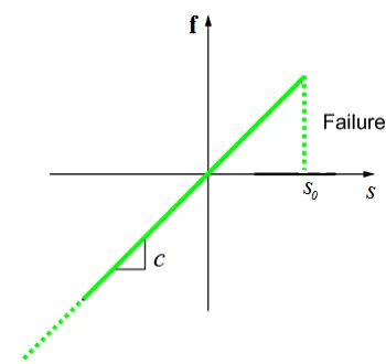
In the case of brittle material behaviour, the peridynamic force and the stretch relationship are shown in Fig. 5.

Fig. 5 PD bond behaviour for brittle materials

The parameter s₀, in Fig. 5, is called critical stretch and if the stretch of a peridynamic bond exceeds this critical value, the peridynamic interaction (bond) is broken. As a result, the peridynamic force between the two material points reduces to zero and the load is redistributed among the other bonds, leading to unguided material failure.

The PD EOM is an integro-differential equation and, in general, it cannot be solved analytically, which means that only an approximated solution can be found. Therefore, numerical techniques for time and spatial integration are usually needed to solve the PD governing equations.

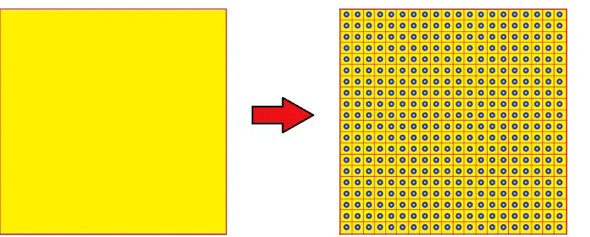
Fig. 6 PD domain discretisation in 2D

For a generic material point x, the spatial integration is performed only over the part of the body that is contained within the horizon of particle x. Therefore, for a generic PD particle x_i, the discretised form of Eq. (1) can be written as

( ) ( )

(

( )

( )

)

( )

t t t V t

ρ x u x =

∑

where M is the number of family members of particle x_i.

4. Peridynamic model of cubic polycrystals

Fig. 7 Voronoi polycrystal

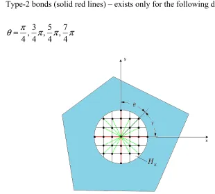
The micro-mechanical PD model of cubic polycrystals is constituted of the following two types of PD bonds (Fig. 8):

• Type-1 bonds (dashed green lines) – exists in all directions (i.e. θ =0 2− π )

• Type-2 bonds (solid red lines) – exists only for the following directions:

3 5 7

, , ,

4 4 4 4

π

θ = π π π

Fig. 8 Type-1 (dashed green lines) and type-2 (solid red lines) bonds for the PD micro mechanical model for a crystal orientation γ equals π/4

measured with respect to the x-axis, while, in general, an algorithm is used to assign a random orientation γ to the grain. As a result of this procedure, when a polycrystalline system of random texture is represented by this model, type-2 bonds will exist in many different directions according to the random orientations of the crystals.

The bond constants for type-1 and type-2 PD bonds can be expressed in terms of the material constants of a cubic crystal,C_ij, by following a procedure similar to that explained in Madenci & Oterkus (2014) [7]. In the case of plane stress condition, the bond constants can be expressed as

2

11 11 12

1 3

11

12( )

T

c c c c

h c π δ

−

=

₍

₎

2

11

4(3 2 )

T

A B

c c c c

c c β β − − = + (5)

where h is the thickness of the structure. The quantities β_A and β_B can be expressed as

1 A q

A ij j

j V β ξ = =

∑

B ij j

j V

β ξ

=

=

∑

where subscript A is associated with directions ,5 4 4

π

θ = π , whilst subscript B is

associated with directions 3 ,7 4 4 θ = π π.

In Eq. (6), i and j refer to a generic particle and its neighbour, respectively, j

V denotes the volume of particle j, ξ_ij is the initial length of the bond between particles i and j, and q_A and q_B represent the number of PD bonds along the directions associated with A and B, respectively.

0

4 9

c G s

E π

δ

= (7)

where E is the Young’s modulus. In case of linear elastic material, the critical energy release rate

G

K

E K G_c Ic

2

5. Peridynamic pitting corrosion model based on Chen & Bobaru (2015) [2]

The pitting corrosion damage model used in this study is based on the model developed by Chen & Bobaru (2015) [2]. According to this model, metal dissolution is predicted by using a modified Nerst-Planck equation (NPE). The NPE is a mass conservation equation that describes the motion of charged chemical species in a fluid under the effect of concentration gradients (diffusion), electric field (migration) and fluid velocity (convection). In this regard, the flux N_i in [mol/(m2/s)] of the generic species ‘i’ can be written as [2,4]

F R

i i i i i i i

convection diffusion electro migration

D C n D C C

T φ

−

= ∇ − ∇ +

N U

(9)

where D_i in [m2/s] is the diffusion coefficient, C_i is the concentration in [mol/m3] of the species “i”, F in [C/mol] is the Faraday constant, R in [J/(mol K)] is the universal gas constant, n_i is the valence number, ϕ in [V] or [J/C] is the electric potential and U in [m/s] is the flow velocity. The conservation of mass can be written as [4]

i

i C

t

∂ _=−∇⋅

∂ N (10)

where t in [s] is time and ∇ ⋅ is the divergence operator.

The majority of pitting corrosion models available in the literature focuses on the motion of chemical species inside the electrolyte solution. However, recent experimental studies have revealed the existence of a ‘wet region’ at the solid/liquid interface of the corrosion pit, where the motion of chemical species can occur. In order to capture this process, Eq. (10) is used to predict the motion of metal cations

+

Men _{in both the electrolyte solution and the solid with the following simplifications}

For the motion within the solution, the electromigration and convective terms in Eq. (9) are included inside the diffusion coefficient, which is now called effective diffusion coefficient in the liquid D_ld. Therefore, the governing equation used to predict the motion of metal cations within the electrolyte solution is given by the following modified version of the Nernst-Planck equation (vid. Eq. (9-10)):

(

)

MI

ld MI ld MI C

D C D C

t

∂ _{=−∇⋅ ∇ = ∇}

∂ (11)

where, in this case, C_MI refers to the metal concentration inside the electrolyte solution.

For the motion within the solid, the velocity of the fluid diffusing inside the pores of the metal is neglected and, therefore, the convection term in Eq. (9) is not considered. The effect of the electromigration term in Eq. (9) is included inside the diffusion coefficient, which is now called effective diffusion coefficient in the solid

sd

D . Therefore, the governing equation used to describe the motion of metal cations within the solid is given by the following modified version of the Nernst-Planck equation (vid. Eq. (9-10)):

(

)

MI

sd MI sd MI

C

D C D C

t

∂ _{=−∇⋅ ∇ = ∇}

∂ (12)

where, in this case, C_MI refers to the metal concentration inside the solid.

In order to obey Faraday’s laws of electrolysis, the effective diffusion coefficient in the solid is expressed as a function of the overpotential η as [2]

F R ( ) (0)

n T

sd sd sd

D D D e

α η

η

= = (13)

When the concentration of metal ions in the liquid reaches the saturation value

sat

C , a salt film precipitates at the liquid/solid interface, which means that the concentration of metal ions in the liquid cannot be greater than the saturation value. Therefore, when the concentration value of the generic node is greater than C_sat, then the node is considered to be in solid phase. On the contrary, when the concentration value is smaller than C_sat, then the node is considered to be in liquid phase.

The peridynamic governing equation for metal dissolution can be written as [8-10]

( )

( )

(

)

d

( , ) , , , , , , d

MI MI MI

H

C t =

∫

x'

x x x x x ₍₁₄₎

where C_MI( , )x t is the time derivative of metal ions concentration associated with the generic material point x. In Eq. (14), the peridynamic function

( )

( )

(

)

d MI , , MI , , , ,

f C x t C x′t x x′ t is called metal dissolution response function and is defined as

d

( , ) ( , )

MI MI

MI

C t C t

f =d ′ −

′ −

x x

x x (15)

in which the peridynamic metal ions diffusion bond constant d_MI can be expressed in terms of the effective diffusion coefficient as [2]

(2 ) 4 ₂eff MI D D d h π δ ⋅ =

⋅ ⋅ (16)

2

2

sd i sat j sat

ld i sat j sat

sd ld

eff i sat j sat

sd ld

sd ld

i sat j sat sd ld

D if C C and C C

D if C C and C C

D D

D if C C and C C

D D

D D

if C C and C C

D D

> > ⎧

⎪ _{< <}

⎪ ⎪⎪ ⋅ ⋅ =⎨ ≤ ≥ + ⎪ ⎪ ⋅ ⋅ ⎪ ≥ ≤ + ⎪⎩ (17)

The PD model of pitting corrosion consists of mechanical bonds overlapped by diffusion bonds. The former bonds are aimed to capture the subsurface mechanical damage reported in recent experimental studies. For this purpose, a damage index,d( , )x t , is defined for each node as

( , ) f

tot N d t N = x (18)

where N_f and N_tot are the number of failed bonds and the total number of bonds attached to the node at x, respectively. At the beginning of the simulation, all the nodes belonging to the solid body have a concentration value C_MI( , )x t equal to

solid

C , which means no corrosion. Therefore, in this condition, all the mechanical bonds connected to xare intact and its damage d( , )x t index is null. On the contrary, when C_MI( , )x t becomes smaller than C_liquid, the node at x changes its phase from solid to liquid, which means complete metal dissolution. Therefore, in this condition, all the mechanical bonds connected to x are broken and the damage index has a unit value. As suggested in Chen & Bobaru (2015) [2], the damage index

( , )

d x t can therefore be written as a function of the nodal concentration CMI( , )x t as

( , ) ( , ) solid MI

solid sat

C C t

d t C C − = − x x ₍₁₉₎

1

1 1

i r

t solid sat C P

d₋ C C

⎛ Δ ⎞

= _{⋅⎜ ⎟}

− _⎝ − _⎠ (20)

where d_t−1 represents the value of the damage index at the previous time step, and

i

C

Δ is the difference in nodal concentration between the previous time step and the current time step. Once Pr is calculated, a random number in the range [0,1] is generated for each bond. If the random number is smaller than Pr, then the mechanical bond is broken and the value of the damage index is updated.

Procedure to obtain realistic pit morphologies

In reality, corrosion pits can have complex geometries. In order to obtain realistic pit morphologies, the following procedure can be followed:

1. The region of the domain where the pit is expected to propagate is selected in the model.

2. For all the nodes that are located outside of this region, an artificial effective coefficient of diffusion in the metal *

sd

D is used. The ratio between * sd D and sd

D is always smaller than 1 and is called “coefficient of pit morphology”

pm c : * 1 sd pm sd D c D

= < (21)

6. Pit-to-crack transition

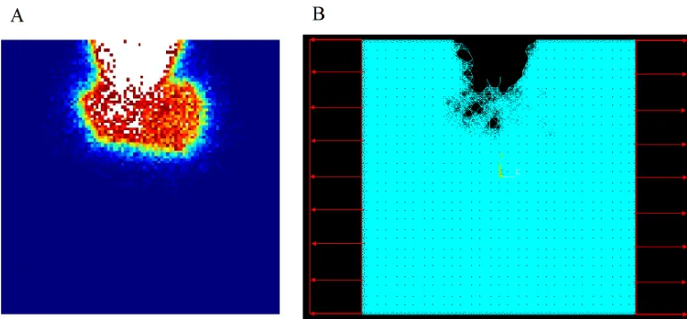
Once the corrosion pit has penetrated inside the body of the metal, a tensile load is applied to the structure and the resulting pit-to-crack transition is observed (second phase). Pitting corrosion is predicted by using the PD pitting corrosion model described in Section 5, while the PD micro-mechanical model described in Section 4 is used to predict intergranular crack propagation. Therefore, the present model is created by coupling the two PD models mentioned above. Apart from the already discussed advantages of these two models, an additional benefit of such an approach is the possibility to remove the assumption that the pit-to-crack transition has to occur at the pit base. To the best of the author’s knowledge, no PD model of pit-to-crack transition is currently available in the literature. Therefore, the numerical model described in this study is the first of its kind.

Fig. 9 The two phases of the pit-to-crack transition model for the case of subsurface pit: damage index map produced at the end of the first phase of the analysis (A), corrosion damage and mechanical boundary condition applied to the body at the beginning of the second phase of the analysis (B)

7. Numerical results

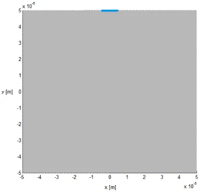
0.1 mm x 0.1 mm and thickness 1 µm. The following boundary condition is applied to the blue region of length 6 µm in Fig. 10: C x t( , ) 0= .

Fig. 10 Model for the first phase of the pit-to-crack transition analysis: metal (grey colour) and corrosive solution (blue colour)

The material and environment are austenitic stainless steel grade 304 exposed to 1M NaCl aqueous solution. The plate is discretised with 100 x 100 PD nodes and the resulting value of grid spacing and horizon radius are Δ= µ1 m and δ = µ3 m, respectively. At the beginning of the simulation, all the nodes belonging to the metal have a concentration of metal ions equal to C_solid. Three different pit morphologies, i.e. wide and shallow pit, subsurface pit and undercutting pit, and one value of applied overpotential, i.e. η = 0.2 V, are considered.

Concerning the second phase of the analysis, i.e. crack propagation, the microstructure of the material is constituted of 50 randomly oriented crystals and the following values of material constants, density and fracture toughness of the material are considered: _c11=204.6 GPa, _c12=137.7 GPa, _{ρ =7880 Kg / m}3 _and

70 MPa m

Ic

The time step size has to be small enough to capture the full dynamic characteristic of the problem and a time step size of dt=0.5 µs was found to be appropriate. Only the bonds crossing the grain boundary of the material are allowed to break, therefore modelling intergranular fracturing only.

Fig. 11 Pit-to-crack transition for the case of wide and shallow pit

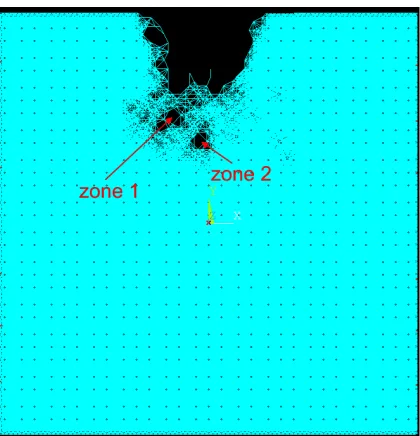
Fig. 12 Pit-to-crack transition for the case of subsurface pit

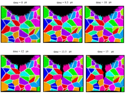
The last pit morphology investigated in this study is the undercutting pit. As shown in Fig. 14, pit-to-crack transition occurs around time = 10 µs at the lower end of the left pit shoulder. At this time, it is also possible to notice the vertical contraction of the plate caused by horizontal opening load and the Poisson’s effect. As time goes by, the crack continues to propagate along the grain boundaries of the material. Around time = 14 µs, a secondary internal crack nucleates in proximity to the lower right edge of the plate.

Fig. 14 Pit-to-crack transition for the case of undercutting pit

8. Conclusions

to predict intergranular crack propagation. Three different pit morphologies, i.e. wide and shallow pit, subsurface pit and undercutting pit, are considered. For the wide and shallow pit case, the pit-to-crack transition takes place at the the pit base. On the other hand, pit-to-crack transition occurs at the left corner of the pit base for the subsurface pit case. Moreover, a subsurface crack nucleates which remains subsurface due to the shielding effect provided by initial corrosion damage. In the final case, i.e. undercutting pit, pit-to-crack transition occurs at the lower end of the left pit shoulder.

field on the pitting evolution process since stress field often enhances metal dissolution. In this study, the pit evolution and crack propagation phases are assumed to be uncoupled. A more comprehensive model can be obtained by developing a fully coupled model. Finally, comparing numerical results against experimental results is beneficial. In this study, a randomly generated microstructure is used as a standard procedure. However, for comparison against experimental results, the microstructural information about grain sizes, grain orientations, etc. should also be available from experiments.

References

[1] Bobaru, F. & Hu, W., 2012. The meaning, selection, and use of the peridynamic horizon and its relation to crack branching in brittle materials.

International Journal of Fracture, 176, pp.215–222.

[2] Chen, Z. & Bobaru, F., 2015. Peridynamic modeling of pitting corrosion damage. Journal of the Mechanics and Physics of Solids, 78, pp.352–381. [3] De Meo, D., Zhu, N., Oterkus, E., 2016. Peridynamic Modeling of Granular

Fracture in Polycrystalline Materials. ASME Journal of Engineering Materials

and Technology, Vol. 138(4), 041008.

[4] Gavrilov, S., Vankeerberghen, M., Nelissen, G., Deconinck, J., 2007. Finite element calculation of crack propagation in type 304 stainless steel in diluted sulphuric acid solutions. Corrosion Science, 49, pp.980–999.

[5] Horner, D. A., Connolly, B. J., Zhou, S., Crocker, L., Turnbull, A., 2011. Novel images of the evolution of stress corrosion cracks from corrosion pits.

Corrosion Science, 53(11), pp.3466–3485.

[6] Kondo, Y., 1989. Prediction of fatigue crack initiation life based on pit growth.

[7] Madenci, E. & Oterkus, E., 2014. Peridynamic theory and its applications. Springer.

[8] Oterkus, S., Madenci, E. and Agwai, A. 2014a. Peridynamic thermal diffusion.

Journal of Computational Physics, 265, pp.71–96.

[9] Oterkus, S., Madenci, E. and Agwai, A. 2014b. Fully coupled peridynamic thermomechanics. Journal of the Mechanics and Physics of Solids, 64, pp.1– 23.

[10] Oterkus, S., Madenci, E., Oterkus, E., Hwang, Y., Bae, J., Han, S., 2014c. Hygro-Thermo-Mechanical Analysis and Failure Prediction in Electronic Packages by Using Peridynamics. , pp.973–982.

[11] Pidaparti, R. M. & Patel, R. K., 2010. Investigation of a single pit/defect evolution during the corrosion process. Corrosion Science, 52(9), pp.3150– 3153.

[12] Pidaparti, R. M. & Patel, R. R., 2008. Correlation between corrosion pits and stresses in Al alloys. Materials Letters, 62, pp.4497–4499.

[13] Pidaparti, R. M. & Patel, R. R., 2011. Modeling the Evolution of Stresses Induced by Corrosion Damage in Metals. Journal of Materials Engineering

and Performance, 20(October), pp.1114–1120.

[14] Pidaparti, R. M. & Rao, A. S., 2008. Analysis of pits induced stresses due to metal corrosion. Corrosion Science, 50, pp.1932–1938.

[15] Rajabipour, A. & Melchers, R. E., 2013. A numerical study of damage caused by combined pitting corrosion and axial stress in steel pipes. Corrosion

[16] Silling, S. A., 2000. Reformulation of elasticity theory for discontinuities and long-range forces. Journal of the Mechanics and Physics of Solids, 48, pp.175– 209.

[17] Ståhle, P., Bjerkén, C. & Jivkov, A.P., 2007. On dissolution driven crack growth. International Journal of Solids and Structures, 44, pp.1880–1890. [18] Suter, T., Webb, E. G., Bohni, H., Alkire, R. C., 2001. Pit initiation on stainless

steels in 1 M NaCl with and without mechanical stress. Journal of the

Electrochemical Society, 148, pp.B174–B185.

[19] Turnbull, A., Horner, D. A., Connolly, B. J., 2009. Challenges in modelling the evolution of stress corrosion cracks from pits. Engineering Fracture

Mechanics, 76(5), pp.633–640.

[20] Turnbull, A., McCartney, L. N., Zhou, S., 2006. A model to predict the evolution of pitting corrosion and the pit-to-crack transition incorporating statistically distributed input parameters. Corrosion Science, 48, pp.2084–2105. [21] Turnbull, A., McCartney, L.N., Zhou, S., 2006. Modelling of the evolution of stress corrosion cracks from corrosion pits. Scripta Materialia, 54, pp.575–578. [22] Turnbull, A., Wright, L., Crocker, L., 2010. New insight into the pit-to-crack transition from finite element analysis of the stress and strain distribution around a corrosion pit. Corrosion Science, 52(4), pp.1492–1498.

[23] Turnbull, A., 2014. Corrosion pitting and environmentally assisted small crack growth. In Proceedings of the Royal Society.

[24] Zhu, L. K., Yan, Y., Qiao, L. J., Volinsky, A. A., 2013. Stainless steel pitting and early-stage stress corrosion cracking under ultra-low elastic load.