Submission Number: EB-19-00266
Is tail risk the missing link between institutions and risk?
Bertrand Groslambert
SKEMA Business School – Université Côte d'Azur, France
Devraj Basu
Wan ni Lai
Strathclyde University, Glasgow, UK
SKEMA Business School – Université Côte
d''Azur, France
Abstract
This paper examines the link between risk and institutional quality, an
unresolved issue in finance. Our hypothesis is that institutions affect risk
through extreme events and not through volatility. We focus on relative
tail risk with an original approach that is able to estimate historical tail
risk with greater precision. Using international stock market data, we
show that tail risk is stable over time, unlike volatility. We find that tail
risk captures the relation between risk and institutional quality better than
volatility. Better governance substantially reduces the probability of
extreme events.
We thank Luc Bauwens, Gaël Leboeuf, Florencio Lopez-de-Silanes and Piet Sercu, for their helpful comments and suggestions.
1.
Introduction
The link between a country’s institutional environment and its economic activity is firmly established, but the question of the mechanisms of transmission is still open to alternative interpretations (Spolaore and Wacziarg 2013). Following Ramey and Ramey (1995), many researchers empirically established that risk is detrimental to growth at least in a cross-country setting. Then, a natural way to investigate the question of how institutions affect economic outcomes is through the effect of institutions on risk. In that respect, a large body of literature has examined the relation between institutional framework and volatility-based risk measures. However, this stream of research has not delivered conclusive results so far and offers contradictory outcomes. In this paper, we assess the distribution of extreme risk across the cross-section of international stock markets and revisit the debate over institutions and risk by exploring a new channel that could provide the missing link between a country’s institutional quality and its economic outcomes—namely, tail risk.
The existing research on the nature of the relation between institutional qualities and risk, uses volatility or volatility-based risk measures. On the one hand, Johnson et al. (2000), Morck et al. (2000), Acemoglu et al. (2003), Jin and Myers (2006) and Hutton et al. (2009) broadly find that better institutions and transparency are associated with low levels for the volatility-based risk measures. On the other hand, Dasgupta et al. (2010), Griffin et al. (2010), and Bartram et al. (2012) find either no relation or an opposite relation between these characteristics. This might be because of the fluctuating and time-varying nature of volatility, as observed in Bekaert and Harvey (1997), which is difficult to reconcile with the enduring pervasiveness of institutions (Glaeser et al., 2004; La Porta et al., 2008). Following on Acemoglu et al. (2017) who show that aggregate volatility and macroeconomic tail risks differ in nature, we investigate whether tail risk is a better candidate than volatility for linking risk and durable institutional characteristics.
First, we investigate the stability of tail risk and volatility over the period 1994-2014. Our results show that the tail indices have remained stable over this period, but we reject the hypothesis of stability in volatility for 80% of countries. This suggests that the slow varying structural factors related to institutional quality are more likely to reflect through tail risk than volatility. Furthermore, we also find that tail risk is orthogonal to volatility in the cross section, revealing that the two measures capture different aspects of country risk. We extend the emerging stream of literature, including Gabaix (2008), Kelly and Jiang (2014) and Acemoglu et al. (2017), on the importance of tail risk in economics and finance by showing that it has different informational content from volatility as a measure of risk at a country level. Our methodology complements Straetmans and Candelon (2013), and Ibragimov et al. (2013) by using a more precise tail index estimator, and extends their work by using a larger sample of countries.
(2000), Acemoglu et al. (2003), and Malik and Temple (2009), who focus on the link between volatility and institutions.
The paper proceeds as follows: Section 2 describes the empirical model, the methods for estimating tail risk and the data. Section 3 presents the results and Section 4 concludes.
2.
Methods and data
2.1. Empirical model and sample construction
To test the effect of institutional quality on respectively tail risk and volatility, we estimate the following cross-sectional model:
= + + + (1)
where is the risk level of stock market i, alternatively measured by its tail risk or its volatility. is the institutional quality variable of country i, is the vector of control variables of country i, and is the error term.
Our initial data set contains daily returns for all stock market indexes across the world that are consistently available in the Bloomberg database since 1994. We retain this starting date to obtain a sufficient number of markets and daily observations per market, especially among emerging countries. If several indexes are available for one country, we retain the index with the highest number of observations. Japan, the United Kingdom, and the United States have several indexes with the same number of observations, so we keep the most comprehensive index for each of these countries (respectively the Topix, FTSE all-share, and S&P 500 indexes). We keep all available countries and only drop stock markets with fewer than 500 observations. This constitutes an initial sample of 89 countries.
2.2. Estimating the tail exponents
Estimating tail risk is an arduous task. Several methods exist for estimating the tail exponent, starting with methods such as the log-log linear regression and the Hill estimator (Hill 1975) as well as more recent techniques based on wavelet analysis (Chen et al. 2018)1.
Unfortunately, they are all very sensitive to the number of observations and require very large dataset for obtaining precise estimates. This raises concerns on the validity of these estimates and makes their use difficult in practice. To address this measurement issue, we take advantage of the fact that we are only interested in the relative ranking and magnitude of the tail risk across countries, and are not concerned by the absolute value of the tail index. Therefore, we can rely on other tools for estimating the relative tail risk. For that, we alternatively assume that returns follow a stable distribution in their tails and estimate the indices with the McCulloch (1986) method instead of using the traditional Hill’s (1975) estimator. Through a Monte Carlo simulation, we establish that the McCulloch estimator is much more precise than the traditional Hill estimator at estimating relative tail risk (see Appendix A). The mathematical justification for this approach is based on the result that non-Gaussian stable laws asymptotically converge to power laws in the
tail, and the approximation seems justified in our case, as our focus is on the cross-sectional variation of the tail indices rather than the precise estimation of individual tail exponents.
As our aim is to understand the difference in tail risk across countries, we focus on the country-specific tail risk. We remove systematic or common factors from the country stock market returns and isolate the country-specific components of the tail index. From the various global risk factors presented in the literature of international asset pricing models, we consider the world market portfolio in our study as the common factor. Recognizing the particular exposure of emerging markets to the price of natural resources, we also follow Harvey (1995) and take into account three additional world risk factors that capture the major part of commodity markets. We regress the country stock market returns on the Bloomberg Energy index, the Bloomberg Precious Metals index, the Bloomberg Industrial Metals index, the Bloomberg Agriculture index, and the MSCI All Countries World index. We then use the residuals from this regression to estimate country-specific tail risk2.
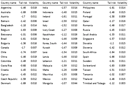
[image:4.595.88.508.413.705.2]A lower tail index means fatter tails and, consequently, more tail risk. To make the reading of the tables more intuitive, we define the tail risk coefficient as the negative of the tail index. Then, we perform cross-section regressions using the estimates of the tail risk coefficients as dependent variables on our set of explanatory variables. Table 1 presents the tail risk estimates and the volatility over the period 1994-2014.
Table 1. Tail risk and volatility.
This table reports the tail risk estimates and the volatility estimates over the period 1994-2014.
Country name Tail risk Volatility Country name Tail risk Volatility Country name Tail risk Volatility
Argentina -1.46 0.019 India -1.57 0.014 Philippines -1.61 0.014
Australia -1.69 0.009 Indonesia -1.48 0.015 Poland -1.46 0.015
Austria -1.7 0.011 Ireland -1.61 0.011 Portugal -1.58 0.009
Bahrain -1.42 0.006 Israel -1.59 0.012 Qatar -1.17 0.016
Bangladesh -1.18 0.014 Italy -1.52 0.010 Romania -1.46 0.017
Belgium -1.63 0.009 Ivory Coast -1.27 0.008 Russia -1.45 0.023 Botswana -1.01 0.006 Kazakhstan -1.12 0.026 Saudi Arabia -1.33 0.011
Brazil -1.61 0.020 Kenya -1.46 0.009 Singapore -1.57 0.010
Bulgaria -1.36 0.016 Korea, South -1.44 0.016 Slovakia -1.2 0.015
Canada -1.7 0.007 Kuwait -1.47 0.009 Slovenia -1.42 0.012
Chile -1.74 0.007 Laos -1.34 0.013 South Africa -1.64 0.010
China -1.46 0.019 Latvia -1.46 0.010 Spain -1.66 0.010
Colombia -1.49 0.013 Lebanon -1.21 0.011 Sweden -1.61 0.011
Costa Rica -0.68 0.018 Malaysia -1.39 0.012 Switzerland -1.63 0.009
Croatia -1.45 0.011 Malta -1.26 0.009 Taiwan -1.51 0.013
Cyprus -1.45 0.022 Mauritius -1.35 0.008 Tanzania -1.02 0.007
Czech Republic -1.59 0.012 Mexico -1.53 0.012 Thailand -1.46 0.015 Denmark -1.69 0.010 Mongolia -1.07 0.044 Trinidad and Tobago -1.12 0.003
2 Five countries display tail indices below one, implying distributions with infinite means, which is not reliable. To
Country name Tail risk Volatility Country name Tail risk Volatility Country name Tail risk Volatility
Ecuador -0.5 0.014 Morocco -1.42 0.007 Tunisia -1.61 0.006
Egypt -1.47 0.014 Namibia -1.71 0.012 Turkey -1.47 0.024
Estonia -1.32 0.014 Netherlands -1.56 0.009 Ukraine -1.35 0.020
Finland -1.47 0.015 New Zealand -1.69 0.011 United Arab Emirates -1.47 0.017
France -1.67 0.009 Nigeria -1.39 0.010 United Kingdom -1.7 0.007
Germany -1.61 0.010 Norway -1.67 0.011 United States -1.55 0.006
Ghana -0.75 0.010 Oman -1.2 0.009 Venezuela -1.34 0.017
Greece -1.55 0.016 Pakistan -1.38 0.015 Vietnam -1.46 0.015
Hong Kong -1.47 0.015 Palestine -1.17 0.013 Zambia -0.98 0.013 Hungary -1.66 0.015 Panama -0.97 0.006
Iceland -1.44 0.010 Peru -1.53 0.012
2.3. Explanatory variables
These are of two types of explanatory variables: those that deal with the economic and financial environment and those that deal with the quality of institutions. The first group of variables can be interpreted as barriers that lead to differences in stock market returns.
As Glaeser et al. (2004) note, when countries become richer, they are likely to improve their institutions. We therefore control for the log of GDP per capita in all regressions. In addition, countries with less developed financial systems tend to have larger market-wide fluctuations. Higher stock market synchronicity is a possible reason for these fluctuations (Morck et al., 2000). Weak financial development can also represent a barrier to market integration and explain cross-sectional variations in tail risk. Consequently, we use market capitalization as a percentage of GDP and stocks traded as a percentage of GDP to capture the degree of stock market development. Infrequent trading and insufficient liquidity are other sources of possible wide fluctuations. Stocks traded as a percentage of market capitalization (stock turnover ratio) control for the activity and liquidity of the market. These three variables provide information about the maturity of the financial system. All else being equal, we expect that more mature markets function more smoothly and have a lower tail risk. Finally, we take the log of number of stocks to control for the higher diversification of larger markets due to the law of large numbers.
We also include the trade-to-GDP ratio, which controls for the country's economic openness. External shocks can generate additional risk, and more opened countries could have a higher tail risk. Last, we consider financial openness and use the Chinn and Ito (2008) index. Financial liberalization could improve international risk sharing and help reduce tail risk. Conversely, it could provoke abrupt capital movements and increase extreme risk.
Marshall et al. (2015). However, even though this indicator theoretically offer better measures of the quality of institutions, it may not give a reliable picture of the institutional environment, if not actually and properly enforced. Addressing this problem, Chong et al. (2014) developed an indicator based on the quality of the universal postal service across 159 countries. They show that this measure represents an objective and actual proxy for measuring government efficiency. We retain this indicator as an objective measure of institutional quality. Finally, we also consider Kaufmann et al.’s (2010; hereinafter KKM) government effectiveness indicator as subjective measures of institutional quality.
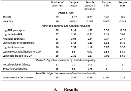
[image:6.595.74.519.331.641.2]Table 2 gives the summary statistics. Table B.1 in the appendix gives the sources of the variables.
Table 2. Summary statistics for tail risk, economic and financial variables, and institutional quality variables.
This table reports summary statistics for risk dependent variables (panel A), economic and financial variables (panel B), and objective and subjective institutional quality variables (panels C and D). All variables are defined in the appendix.
Number of countries
Sample mean
Sample standard deviation
Sample min
Sample max
Panel A: Risk
Tail risk 89 -1.37 0.23 -1.66 -0.5
Volatility 89 0.012 0.005 0.003 0.044
Panel B: Economic and financial variables
Log GDP per capita 88 9.14 1.32 6.36 11.33
Log trade to GDP 87 4.36 0.51 3.13 5.93
Financial openness 87 0.94 1.34 -1.34 2.44
Log number of listed stocks 86 5.12 1.49 2.14 8.72
Log stock turnover 86 3.35 1.19 0.87 5.36
Log market capitalization to GDP 86 3.6 0.92 1.54 5.89
Log stocks traded to GDP 86 2.31 1.87 -1.98 5.69
Panel C: Objective measures of institutional quality
Postal service efficiency 87 0.7 0.3 0 1
Executive Constraints 85 5.6 1.73 1 7
Panel D: Subjective measures of institutional quality
Government effectiveness 88 0.53 0.89 -1.02 2.13
3.
Results
3.1. Tail risk versus volatility risk
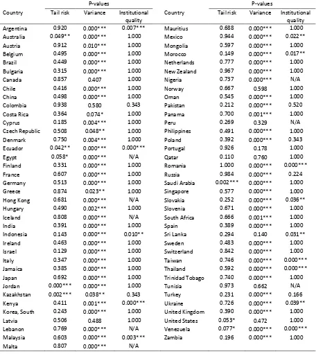
of tail risk using Phillips and Loretan’s (1990) structural change procedure. For volatility risk, we use Levene’s test, which is robust to departure from normality. In order to reduce the risk that our results be driven by a lack of power of the tests, we retain a significance criterion of 20%. Results are presented in Table 3.
The hypothesis of tail index stability cannot be rejected at this large 20% level for 81% of the countries and for most countries, p-values are well above that threshold. Thus, we can conclude with some confidence that tail risk remained stable during our sample period even though there was substantial transformation in emerging stock markets at that time. This is in line with Straetmans and Candelon (2013), who empirically test for structural changes in extreme risk on a large set of asset classes across various international markets and do not detect any breaks except for a few emerging currency tails. Focusing on foreign exchange markets, Ibragimov et al. (2013) find similar results. This suggests that long horizon tail risk, while potentially time-variant, exhibits slow variation and is likely to be related to deeper structural factors. We also test the stability of the institutional quality over the sub-periods 1994–2003 and 2004–2014 using the executive constraints variable as objective measure of the institutions. As for tail risk, we find that almost eighty percent of countries exhibit a stable institutional environment at the large threshold of twenty percent.
Table 3. Test of equality across time: 1994–2003 versus 2004–2014.
This table reports the p-values of the test for the equality across time of respectively the tail risk based on the Phillips and Loretan’s (1990) test of equality of tail index, the variance based on the Levene test of equal variance
and the institutional quality based on the t test. Institutional quality is measured by the executive constraints
variable. Fourteen countries have not enough observations for estimating the tail index during the 1994–2003 period, and are not reported here. *** p<0.01, ** p<0.05, * p<0.1.
P-values P-values
Country Tail risk Variance Institutional quality
Country Tail risk Variance Institutional quality Argentina 0.920 0.000*** 0.007*** Mauritius 0.688 0.000*** 1.000 Australia 0.049** 0.000*** 1.000 Mexico 0.944 0.000*** 0.022** Austria 0.912 0.010*** 1.000 Mongolia 0.597 0.000*** 1.000 Belgium 0.495 0.000*** 1.000 Morocco 0.149 0.000*** 0.017** Brazil 0.449 0.000*** 1.000 Netherlands 0.777 0.000*** 1.000 Bulgaria 0.315 0.000*** 1.000 New Zealand 0.967 0.000*** 1.000 Canada 0.857 0.407 1.000 Nigeria 0.737 0.000*** N/A Chile 0.416 0.000*** 1.000 Norway 0.667 0.598 1.000 China 0.498 0.000*** 1.000 Oman 0.545 0.000*** 1.000 Colombia 0.938 0.580 0.343 Pakistan 0.212 0.000*** 0.520 Costa Rica 0.364 0.074* 1.000 Panama 0.700 0.001*** 1.000 Cyprus 0.185 0.004*** 1.000 Peru 0.269 0.329 N/A Czech Republic 0.508 0.048** 1.000 Philippines 0.491 0.000*** 1.000 Denmark 0.750 0.004*** 1.000 Poland 0.392 0.000*** 0.343 Ecuador 0.042** 0.000*** 0.000*** Portugal 0.926 0.178 1.000 Egypt 0.058* 0.000*** N/A Qatar 0.110 0.760 1.000 Finland 0.331 0.000*** 1.000 Romania 1.000 0.000*** 0.000*** France 0.607 0.000*** 1.000 Russia 0.984 0.000*** 0.224 Germany 0.513 0.000*** 1.000 Saudi Arabia 0.002*** 0.000*** 1.000 Greece 0.874 0.023** 1.000 Singapore 0.577 0.000*** 1.000 Hong Kong 0.681 0.000*** N/A Slovakia 0.252 0.000*** 0.036** Hungary 0.490 0.002*** 1.000 Slovenia 0.671 0.000*** 1.000 Iceland 0.808 0.000*** N/A South Africa 0.666 0.001*** 1.000 India 0.391 0.000*** 1.000 Spain 0.389 0.000*** 1.000 Indonesia 0.143 0.000*** 0.010** Sri Lanka 0.294 0.140 0.031** Ireland 0.463 0.000*** 1.000 Sweden 0.483 0.000*** 1.000 Israel 0.129 0.000*** 1.000 Switzerland 0.842 0.000*** 1.000 Italy 0.347 0.000*** 1.000 Taiwan 0.746 0.000*** 0.000*** Jamaica 0.385 0.000*** 1.000 Thailand 0.592 0.000*** 0.000*** Japan 0.692 0.000*** 1.000 Trinidad Tobago 0.740 0.000*** 1.000 Jordan 0.000*** 0.000*** 1.000 Tunisia 0.973 0.662 N/A Kazakhstan 0.002*** 0.038** 0.343 Turkey 0.231 0.000*** 0.166 Kenya 0.411 0.001*** 0.000*** Ukraine 0.726 0.000*** 0.039** Korea, South 0.243 0.000*** 1.000 United Kingdom 0.390 0.000*** 1.000 Latvia 0.506 0.488 1.000 United States 0.053* 0.472 1.000 Lebanon 0.769 0.000*** N/A Venezuela 0.077* 0.000*** 0.000*** Malaysia 0.603 0.000*** 0.003*** Zambia 0.196 0.000*** 1.000
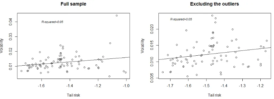
Figure 1 shows the scatter plots between the tail risk estimates and volatility estimates over the full sample period for the countries in our sample and excluding the outliers3. The R-square
[image:9.595.73.515.320.480.2]for these scatter plots is 5%, suggesting that in a cross-sectional setting, volatility and tail risk are orthogonal to each other, thus indicating that tail risk is quite distinct from volatility. This empirical finding provides further justification for our cross-sectional analysis of tail risk on its own. Taken together, these findings show that the behavior of tail risk is very different from that of volatility in our sample period. This result conforms to Acemoglu et al. (2017) who show that aggregate volatility and macroeconomic tail risks differ in nature. Our findings on the orthogonality of tail risk and volatility and the higher persistence of tail risk are in line with those of Bollerslev and Todorov (2011) who also find that tail risk is compensated differently from variance. The time-varying measure of volatility is not the same in nature as deep structural factors that drive institutions. The latter conform better to the more stable nature of tail risk, which manifests occasionally through extreme events.
Fig. 1. Scatter plots for the tail risk estimates and the volatility estimates
3.2. Cross-sectional determinants of tail risk
We use a cross-sectional regression because the tail risk estimate, which is the dependent variable, requires observations gathered over a long time horizon and because some variables do not vary much over time. In estimating eq. (1), it is possible that our institutional variables are endogenous due to either a problem of omitted variables or model misspecification. Endogeneity could also be caused by a problem of simultaneity, if the quality of the institutions is jointly determined with extreme risks, or reverse causality, if countries more prone to extreme events adopted certain types of institutions. Finally, it could arise from measurement errors because of the difficulty in precisely estimating institutional quality. We address these issues by implementing an instrumental variable (IV) technique. In our case, we have two sets of institutional measures that are potentially endogenous: objective and subjective. The source of their endogeneity certainly differs between the two sets, particularly because the subjective KKM variable may be more exposed to measurement errors. Therefore, we do not use the same instruments for objective and subjective measures of institutions.
3 Based on the Cook’s distance cut-off of 4/n, we identified Botswana, Kazakhstan, Mongolia, Tanzania and
Although the debate about the respective influence of geographic endowments versus human capital on economic growth is not yet settled, the literature shows a relation between these factors and the institutional quality of a country, either direct or indirect. We borrow from this literature to find IVs that satisfy the conditions of being highly related to the objective measures of institutional quality and satisfying the exclusion restriction. The geographic size of a country is the first potential instrument that we consider. Following Olsson and Hanson (2011), we argue that the larger a country, the more difficult it is to implement good institutions equally over the total area of the country. The second instrument that we retain is the share of descendants of Europeans, in line with Putterman and Weil (2010). The argument follows Acemoglu et al.’s (2001) line of reasoning. Europeans who settled in regions with a favorable biogeographic environment developed a good institutional framework, whereas European settlers in an unfavorable biogeographic environment implemented bad and extractive institutions. Therefore, the share of European descendants is likely to determine the quality of institutions. We apply standard over-identification tests and find that the excluded instruments are independent of the error process.
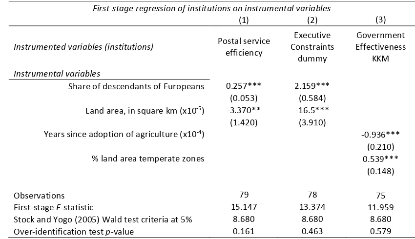
[image:10.595.81.506.468.713.2]Regarding the subjective measure of institutions, the first instrument that we retain is the number of years elapsed since the adoption of agriculture, in line with Putterman and Weill (2010). Following Putterman (2008), we argue that the timing of transitions to agriculture influences the capacity of communities to organize as states and to invent good institutional models, through the accumulation of “statehood experience.” We also consider the percentage of land area in temperate zones as instrument. Rodrik et al. (2004) show that geographic endowments such as temperate versus tropical location determine the quality of institutions but do not affect economic output directly. Table 4 presents the results of the first-stage IV regression. All our instruments have F-statistics above ten and successfully pass the Stock and Yogo’s (2005) Wald test criteria at the 5% level.
Table 4. IV (LIML) first-stage regression for various measures of institutions.
First-stage regression of institutions on instrumental variables
(1) (2) (3)
Instrumented variables (institutions) Postal service
efficiency
Executive Constraints
dummy
Government Effectiveness
KKM
Instrumental variables
Share of descendants of Europeans 0.257*** 2.159***
(0.053) (0.584)
Land area, in square km (x10-5) -3.370** -16.5***
(1.420) (3.910)
Years since adoption of agriculture (x10-4) -0.936***
(0.210)
% land area temperate zones 0.539***
(0.148)
Observations 79 78 75
First-stage F-statistic 15.147 13.374 11.959
Stock and Yogo (2005) Wald test criteria at 5% 8.680 8.680 8.680
To strengthen our case further, we implement the limited information maximum likelihood (LIML) estimation method, which has a lower bias and lower mean square error than the two-stage least squares method if the sample is small (Stock and Yogo, 2005).
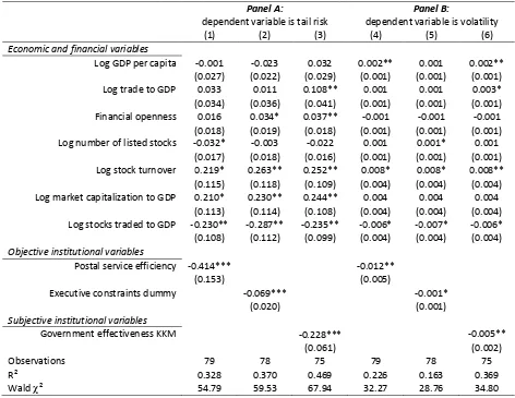
[image:11.595.61.533.334.699.2]The results shown in panel A of Table 5 indicate a strong and significant influence of institutions on tail risk. All measures of institutional quality display a negative significant coefficient at the one-percent level. The marginal effect of institutions on tail risk is very important. For instance, we find that if a country such as Columbia (25th percentile) were to increase its government effectiveness index to the level of Chile (75th percentile), it would reduce by 69% the risk of daily drawdowns of 5% or more.
Table 5. IV (LIML) cross-sectional regression on economic, financial, and institutional variables.
This table shows the results of the second-stage regression for various measures of institutions. The dependent variable is the tail risk of returns in Panel A and the volatility in Panel B. The explanatory variables are the economic, financial and institutional variables. Tail risk is defined as the negative of the tail index of returns. The specifications include a constant not reported in the table. Robust standard errors are in parentheses. *** p<0.01, ** p<0.05, * p<0.1. All variables are defined in the appendix.
Panel A:
dependent variable is tail risk
Panel B:
dependent variable is volatility
(1) (2) (3) (4) (5) (6)
Economic and financial variables
Log GDP per capita -0.001 -0.023 0.032 0.002** 0.001 0.002**
(0.027) (0.022) (0.029) (0.001) (0.001) (0.001)
Log trade to GDP 0.033 0.011 0.108** 0.001 0.001 0.003*
(0.034) (0.036) (0.041) (0.001) (0.001) (0.001)
Financial openness 0.016 0.034* 0.037** -0.001 -0.001 -0.001
(0.018) (0.019) (0.018) (0.001) (0.001) (0.001)
Log number of listed stocks -0.032* -0.003 -0.022 0.001 0.001* 0.001
(0.017) (0.018) (0.016) (0.001) (0.001) (0.001)
Log stock turnover 0.219* 0.263** 0.252** 0.008* 0.008* 0.008**
(0.115) (0.118) (0.109) (0.004) (0.004) (0.004)
Log market capitalization to GDP 0.210* 0.230** 0.244** 0.004 0.004 0.004
(0.113) (0.114) (0.108) (0.004) (0.004) (0.004)
Log stocks traded to GDP -0.230** -0.287** -0.235** -0.006* -0.007* -0.006*
(0.108) (0.112) (0.099) (0.004) (0.004) (0.004)
Objective institutional variables
Postal service efficiency -0.414*** -0.012**
(0.153) (0.005)
Executive constraints dummy -0.069*** -0.001*
(0.020) (0.001)
Subjective institutional variables
Government effectiveness KKM -0.228*** -0.005**
(0.061) (0.002)
Observations 79 78 75 79 78 75
R² 0.328 0.370 0.469 0.226 0.163 0.369
Panel B of Table 5 investigates the relation between institutions and the volatility as dependent variable. The coefficient of regression of institutional variables is significantly negative, but only at the five or ten percent level. We find that if a country such as Columbia (25th percentile) were to increase its government effectiveness index to the level of Chile (75th percentile), it would reduce the daily volatility by 44%.
When looking at the Chi square statistics, we find that the goodness of fit of tail risk models (Panel A) is two times larger than those of volatility models (Panel B). Overall, these results show that institutions are an important determinant of risk across countries. This could explain why Ghysels et al. (2016), who do not consider institutional quality among the possible explaining variables, find low explanatory power in their cross-country regression of conditional skewness.
3.3. Robustness checks
In our base model, we exclude the tail index estimates that are beyond the range usually documented in the literature and retain the McCulloch estimates above one. We test the robustness of our results by taking two alternative samples. First, we use the full sample without excluding any tail index estimate. Second, because our initial sample includes frontier and small emerging markets, our results could be driven by infrequent trading. To address this issue, we also use a sample that excludes the first quartile of countries with the lowest stock turnover. The results of these robustness checks are similar to those presented in the previous sections and available on request.
4.
Conclusion
This paper examines the link between stock market risk and institutional quality, an unresolved issue in the finance and economics literature. We find that volatility and tail risk are uncorrelated in the cross-section. We find a strong empirical relation between tail risk and the quality of institutions even after accounting for economic and financial variables. Overall, it seems that the institutional quality of country is a structural determinant of its tail risk. Conversely, we find a weaker association between institutional quality and volatility. It appears that institutional quality affects risk more through persistent tail risk and less through time-varying volatility. This may help to explain the conflicting results in the existing literature that uses volatility-based measures of risk.
References
Acemoglu, D., Johnson, S., Robinson, J. A. (2001) “The colonial origins of comparative development: an empirical investigation” American Economic Review91(5), 1369-1401.
Acemoglu, D., Johnson, S., Robinson, J., Thaicharoen, Y. (2003) “Institutional causes, macroeconomic symptoms: volatility, crises and growth” Journal of Monetary Economics50(1), 49-123.
Bartram, S. M., Brown, G., Stulz, R. M. (2012) “Why are US stocks more volatile?” Journal of Finance67(4), 1329-1370.
Bekaert, G., Harvey, C. R. (1997) “Emerging equity market volatility” Journal of Financial Economics43(1), 29-77.
Bollerslev, T., Todorov, V. (2011) “Tails, fears, and risk premia” Journal of Finance66(6), 2165-2211.
Chen, Y. T., Sun, E. W., & Yu, M. T. (2018) “Risk assessment with wavelet feature engineering for high-frequency portfolio trading” Computational Economics52(2), 653-684.
Chinn, M. D., Ito, H. (2008) “A new measure of financial openness” Journal of Comparative Policy Analysis 10(3), 309-322.
Chong, A., La Porta, R., Lopez-de-Silanes, F., Shleifer, A. (2014) “Letter grading government efficiency” Journal of the European Economic Association12(2), 277-298.
Dasgupta, S., Gan, J., Gao, N. (2010) “Transparency, price informativeness, and stock return synchronicity: theory and evidence” Journal of Financial and Quantitative Analysis45(5), 1189-1220.
Gabaix, X. (2008) “Variable rare disasters: a tractable theory of ten puzzles in macro-finance”
American Economic Review98(2), 64-67.
Ghysels, E., Plazzi, A., Valkanov, R. (2016) “Why invest in emerging markets? The role of conditional return asymmetry” Journal of Finance71(5), 2145-2192.
Glaeser, E. L., La Porta, R., Lopez-de-Silanes, F., Shleifer, A. (2004) “Do institutions cause growth?” Journal of Economic Growth9(3), 271-303.
Griffin, J. M., Kelly, P. J., Nardari, F. (2010) “Do market efficiency measures yield correct inferences? A comparison of developed and emerging markets” Review of Financial Studies23(8), 3225-3277.
Harvey, C. R. (1995) “Predictable risk and returns in emerging markets” Review of Financial Studies8(3), 773-816.
Hill, B. M. (1975) “A simple general approach to inference about the tail of a distribution” Annals of Statistics3(5), 1163-1174.
Hutton, A. P., Marcus, A. J., Tehranian, H. (2009) “Opaque financial reports, R2, and crash risk”
Journal of Financial Economics94(1), 67-86.
Ibragimov, M., Ibragimov, R., Kattuman, P. (2013) “Emerging markets and heavy tails” Journal of Banking & Finance37(7), 2546-2559.
Jin, L., Myers, S. C. (2006) “R2 around the world: new theory and new tests” Journal of Financial Economics79(2), 257-292.
Kaufmann, D., Kraay, A., Mastruzzi, M. (2010) “The worldwide governance indicators: methodology and analytical issues” World Bank Policy Research Working Paper number 543.
Kelly, B., Jiang, H. (2014) “Tail risk and asset prices” Review of Financial Studies27(10), 2841-2871.
La Porta, R., Lopez-de-Silanes, F., Shleifer, A. (2008) “The economic consequences of legal origins” Journal of Economic Literature46(2), 285-332.
Malik, A., Temple, J. R. (2009) “The geography of output volatility” Journal of Development Economics90(2), 163-178.
Marshall, M. G., Gurr, T. R., Jaggers, K. (2015) “Polity IV project: political regime characteristics and transitions, 1800–2014 dataset” Center for Systemic Peace.
McCulloch, J. H. (1986) “Simple consistent estimators of stable distribution parameters”
Communications in Statistics-Simulation and Computation15(4), 1109-1136.
Morck, R., Yeung, B., Yu, W. (2000) “The information content of stock markets: why do emerging markets have synchronous stock price movements?” Journal of Financial Economics58(1), 215-260.
Olsson, O., Hansson, G. (2011) “Country size and the rule of law: Resuscitating Montesquieu”
European Economic Review55(5), 613-629.
Phillips, P. C., Loretan, M. (1990) “Testing covariance stationarity under moment condition failure with an application to common stock returns” Cowles Foundation for Research in Economics
number 947, Yale University.
Putterman, L. (2008) “Agriculture, diffusion and development: ripple effects of the neolithic revolution” Economica75(300), 729-748.
Putterman, L., Weil, D.N. (2010) “Post-1500 population flows and the long-run determinants of economic growth and inequality” Quarterly Journal of Economics125(4), 1627-1682.
Ramey, G., Ramey, V. A. (1995) “Cross-country evidence on the link between volatility and growth” American Economic Review85(5), 1138-1151.
Rodrik, D., Subramanian, A., Trebbi, F. (2004) “Institutions rule: the primacy of institutions over geography and integration in economic development” Journal of Economic Growth9(2), 131-165.
Spolaore, E., Wacziarg, R. (2013) “How deep are the roots of economic development?” Journal of Economic Literature51(2), 325-369.
Stock, J. H., Yogo, M. (2005) “Testing for weak instruments in linear IV regression” in
Identification and Inference in Econometric Models: Essays in Honor of Thomas J. Rothenberg
by D.W.K. Andrews and J.H. Stock Eds., Cambridge University Press, pp. 80-108.
Sun, W., Rachev, S., & Fabozzi, F. J. (2009) “A new approach for using Lévy processes for determining high‐frequency value‐at‐risk predictions” European Financial Management 15(2), 340-361.