A Memetic Approach to the Solution of
Constrained Min-Max Problems
Gianluca Filippi
Mechanical and Aerospace Engineering University of Strathclyde
Glasgow, UK [email protected]
Massimiliano Vasile
Mechanical and Aerospace Engineering University of Strathclyde
Glasgow, UK [email protected]
Abstract—This paper proposes a novel memetic algorithm for the solution of constrained min-max problems that derive from the optimal design of complex systems under worst-case conditions. In this context the maximisation of a quantity of interest over the space of uncertain variables is required to identify the worst-case scenario (or worst-case solution under uncertainty). An optimal design vector is then identified such that the worst-case value of the quantity of interest is minimised. In the most general case, both maximisation and minimisation are subject to strict feasibility constraints. The ultimate goal of the minimisation problem is to identify the design solution that is feasible for all possible values of the uncertain parameters.
Index Terms—worst case scenario, min-max, epistemic uncer-tainty, benchmark
I. INTRODUCTION
One aspect of Resilience Engineering is the design of systems that are robust against uncertainty of different nature. Different sources of uncertainty are possible: uncertainty on model definition, measurement noise, manufacturing and fab-rication errors, human error, numerical error, etc [1]. All these forms of uncertainty are commonly classified into groups: aleatoryandepistemic. The former group collects irreducible uncertainties while the latter group collects uncertainty due to lack of knowledge and/or subjective probability. Uncertainty can be reduced to aleatory as information increases.
An engineering system can be optimised using a model for the Quantity of Interest(QoI)f that is a function of both decision (or design) variables d and uncertain parametersu:
f =f(d,u), (1)
with d∈D andu∈U, whereD is a design/decision space and U the uncertainty space. Considering, without loss of generality, a minimisation problem, we can now define the worst-case scenario as the uncertainty vector u∗ such thatf attains the maximum value inU. The resulting unconstrained min-max problem then reads as:
min
d∈Dmaxu∈Uf(d,u) (2)
A simple approach to solve Eq. (2) is described in [2] as Best Replay: for a fixed valueu∗,d
minis evaluated minimising
This research has been developed with the partial support of the H2020 MCSA ITN UTOPIAE grant agreement number 722734.
f(d, u∗); then dmin is fixed and f is maximised over u and this two optimisation steps are alternated until convergence is achieved. Another simple approach is in Eq. (3) where the maximum off overu is minimised overd:
mind∈Df(d) s.t.
f(d) = maxu∈Uf(d,u)
(3)
It has been proven, however, that the Best Replay approach often does not converge or it cycles through wrong design candidates. On the other side, the direct approach proposed in Eq. (3) is too computationally expensive. Thus, a lot of effort has gone into developing methods that solve the min-max problems with an affordable computational cost: a number of papers have been published about mathematical programming [3]–[13] and heuristic methods [14]–[17]. Math-ematical programming approaches require strong assumptions on the nature of the function f and tend to be tailored on specific problems. On the other hand heuristic approaches appear to be more flexible. In particular, evolutionary-based algorithms represent a promising alternative to mathematical programming methods. In the existing literature, only few papers could be found that have explored how to deal with constraints in bi-level optimisation. Most of them need to start from some strong assumptions on the nature of constraints and cost functions and have been developed for constrained bi-level problems and not specifically for the treatment of min-max problems [18], [19].
This paper proposes M acM inM ax, an extension of the algorithm presented in [20] to treat min-max problems under strict constraints. In this case the goal is to find a design solution d∗ that is feasible for all values of the uncertain variablesuand minimises the worst case value of the quantity of interest f. In formulas this constrained min-max problem reads:
mind∈Dmaxu∈Uf(d,u) s.t.
maxu∈UC(d,u)≤0
(4)
are shown in Eq. (III-B). Section IV, finally, comments the performance of the algorithm at identifying feasible and robust solutions.
II. A MEMETICMIN-MAXAPPROACH
The algorithm proposed in this paper is inspired by the procedure, alternatingoptimisationandrestorationloops, sug-gested by Shimizu and Aiyoshi [21], [22]. Following this idea, other methods [20], [23] were developed to solve the uncon-strained problem in Eq. (2). M acM inM ax, first introduced in [24], solves, instead, the more general constrained min-max problem defined in Eq. (4). The original contribution of this paper consists in a new benchmark to test constrained min-max algorithms and the extensive testing of M acM inM ax. M acM inM ax is a bi-level optimisation algorithm where the optimisationloop (upper or outer level) minimises the function f over the decision vectordconsidering the worst condition
uA in an subsetAu of the uncertain space (Au⊂U):
min
d∈D
max
uA∈Au
f(d,uA)
. (5)
Therestoration loop(lower or inner level), instead, maximises the objective functionf over the uncertainty vector ufor the design vector d∗ fixed in the optimisation loop:
max
u∈Uf(d
∗,u). (6)
Both loops are considered under the constraint function C. Note that in the case of a vector of constraint functions [C1, ..., Cnc]we consider the scalar:
C(d,u) = nc X
i=1
max(Ci(d,u),0). (7)
The resulting algorithm proceeds as follows:
1) [Optimisation] Given a set of maxima inAu=AfS Ac, from therestorationloop, solve the constrained minimi-sation problem:
mind∈Dmaxu∈Auf(d,u)
s.t.
maxu∈AuC(d,u)≤0
(8)
The solutiond∗ is then saved in an archive Ad. 2) [Restoration] Given the solution of problem (8), d∗,
solve the two maximisation problems:
maxu∈Uf(d∗,u) s.t.
C(d∗,u)≤0
(9)
max
u∈UCi(d
∗,u) ∀i∈[1, ..., nc]T (10)
The solution of Eq. (9),uaf = arg maxu∈Uf(d∗,u)s.t.
C(d∗,u)≤0, from the space of the feasible maxima of f is added to the archive Af. The solutions of Eq. (10),
uac,i= arg maxu∈UCi(d∗,u) ∀ifrom the space of the maxima violation of the constraint C are stored in the archiveAcifmaxu∈UCi(d∗,u)>0. The archiveAu= Af∪Ac is then used in the upper loop to evaluate the
new d∗. Note that Eq. (10) has to be understood as a maximisation for every constraint function in C and not as a vector optimisation. This approach pushes the optimiser to find design solutions that are feasible for all values of the uncertain variables. If a feasible solution cannot be found, the constraints are relaxed by defining the new constraint C∗ = C+ with the minimum constraint violation overU.
The optimisation and restoration loops are repeated one after the other for a prescribed number of iterations and alld∗ and associated maxima inAuare stored in a global archiveAg(for the relationship between the archives please refer to Fig. 1). The global archive is then used to perform a cross-check of the solutions. Given a finite number of iterations, one might obtain a solutiond∗ associated to non-globally optimal value ofue∈Au. In order to mitigate this problem one can evaluate f andC taking multiple pairs d∗,ue taken from the archive Ag.
The overall procedure is summarised in Algorithm 1 where, without loss of generality, a single constraint C is considered. First, the design vectord¯ is initialised and two optimisations over the uncertain domain U are run keeping fixed ¯d (line 1): a constrained maximisation of f and a maximisation of the constraint violation C. The archives - Af, Ac, Ad -are initialised (line 2). Then the inner and outer loops -are alternated until the maximum number of iterations is reached (lines 3-22). In particular, the archiveAdof the design vectors
Algorithm 1 Constrained min-max
1: Initialised¯at random and run uaf = arg maxf(¯d,u)s.t. C(¯d,u)≤0anduac= arg maxu∈UC(¯d,u)
2: Af ={uaf}; Ac={uac};Ad=∅
3: whileNf val< Nmax f val do
4: Outer loop:
5: dmin= arg mind∈D{maxu∈Af∪Acf(d,u)} s.t.
maxu∈Af∪AcC(d,u)≤0
6: Ad=Ad∪ {dmin}
7: Inner loop:
8: uaf = arg maxu∈Uf(dmin,u)s.t. C(dmin,u)≤0
9: uac= arg maxu∈UC(dmin,u)
10: Af =Af∪ {uaf}
11: ifNf val< Nf valrelaxation∨
∃d∈Ad t.c. maxu∈UC(d,u)≤0then
12: ifmaxu∈UC(dmin,u)>0 then
13: Ac=Ac∪ {uac}
14: end if 15: else 16: update
17: A={A\ua|C(dmin,u)≤}
18: ifmaxu∈UC(dmin,u)> then 19: Ac=Ac∪ {ua,C}
20: end if 21: end if 22: end while
Inner Loop
Af Ac Ad
Outer Loop
[image:3.612.52.300.57.485.2]Au Ag
Fig. 1. Diagram of the relationships between the archives in Algorithm 1.
III. TESTINGPROCEDURE
[image:3.612.314.566.300.481.2]The approach to the solution of constrained min-max prob-lems, M acM inM ax, presented in this paper, is here applied to the benchmark in TABLE I and TABLE III using the testing procedure explained in Algorithm 2 that is a generalisation of what presented in [27]. Each problem pi,j corresponds to a combination of the objective function T C-i(d, u) as in TABLE I and a constraint function T CC-j(d, u) as in TABLE III:pi,j=T C-i∧T CC-j. Problems are solved with M acM inM ax for different numbers of maximum function evaluationsNf evalmax and each combination ofpi,jandNf evalmax is repeatedn= 100times (line 3 of Algorithm 2). The solutions, finally, are compared with the exact min-max presented in TA-BLE II and TATA-BLE IV. As suggested in [27], theSuccess Rate SR is used for the comparative assessment of the algorithm performance instead of best value, mean, and variance. SRis
defined as the ratio js
n wherejs is the index of performance as described in lines 5-10 of Algorithm 2. The number of successes ofM acM inM axon the genericpi,jdepends on the tolerances tolf and tolu - on the objective function solution f and on the uncertain vector u respectively - and on the constraint C satisfaction. The condition is given in line 8 and it depends on the errors δpi,j,k
f , δ pi,j,k
u (with references in TABLES II and IV) and onνpi,j,i
c as described in lines 5-7.fopt(pi,j)in line 5 anduopt(pi,j)in line 6 are the reference solutions for the problem pi,j. di,j,k, and ui,j,k in lines 5-6 are the solution vectors calculated with Algorithm 1 at the k-iteration. ¯ui,j,k in line 7 is, finally, the uncertain vector that maximise the constraint C violation with the design solution
di,j,k. tolu is necessary to verify the convergence on the maximisation in the inner loop (restoration in section II) and then to avoid counting as success solution anfi(di,j,k,ui,j,k) close tofopt(pi,j)that is coming from a lucky combination of a wrong maximisation and a wrong minimisation in the outer loop (optimisation in section II).
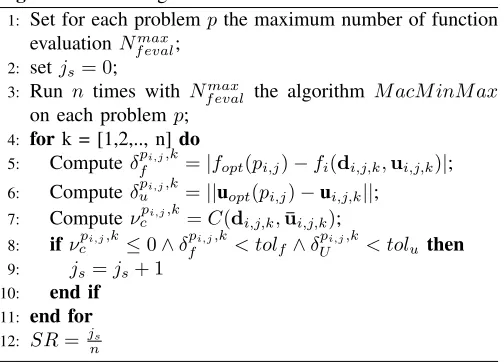
Algorithm 2 Testing Procedure
1: Set for each problempthe maximum number of function evaluationNf evalmax;
2: setjs= 0;
3: Run n times with Nf evalmax the algorithm M acM inM ax on each problemp;
4: fork = [1,2,.., n]do 5: Computeδpi,j,k
f =|fopt(pi,j)−fi(di,j,k,ui,j,k)|;
6: Computeδupi,j,k=||uopt(pi,j)−ui,j,k||;
7: Computeνpi,j,k
c =C(di,j,k,¯ui,j,k);
8: if νpi,j,k
c ≤0∧δpfi,j,k< tolf∧δUpi,j,k< tolu then
9: js=js+ 1
10: end if 11: end for 12: SR= jns
A. Benchmark
Objective functions from TC-1 to TC-6 are convex-concave test functions defined in Chapter5 of [25] and used in [23]. Functions from TC-7 to TC-12 are selected from [16], [17], [26]. TC-13 is a modification of the Rastrigin function where half of the variables are design parameters and the others are epistemic uncertainties. The dimensions of TC from TC-1 to TC-12 range fromdimd = 1anddimu= 1up to dimd= 4 anddimu= 3; dimensions of TC-13 can go from 1 to infinite and is here kept up to dimd = 3 and dimu = 3. Refer-ence solutions for pi,1 and pi,2 are presented in TABLE II:
TABLE I
TEST CASES FOR THE OBJECTIVE FUNCTIONf
name objective function TC
TC-1 f(d, u) = 5(d2
1+d22)−(u21+u22) +d1(−u1+u2+ 5) +d2(u1−u2+ 3) TC-2 f(d, u) = 4(d1−2)2−2u21+d21u1−u22+ 2d22u2
TC-3 f(d, u) =d4
1u2+ 2d31u1−d22u2(u2−3)−2d2(u1−3)2 TC-4 f(d, u) =−P3
i=1(ui−1)2+P2i=1(di−1)2+u3(d2−1) +u1(d1−1) +u2d1d2 TC-5 f(d, u) =−(d1−1)u1−(d2−2)u2−(d3−1)u3+ 2d21+ 3d22+d23
TC-6 f(d, u) =u1(d21−d2+d3−d4+ 2) +u2(−d1+ 2d22−d23+ 2d4+ 1) +d3(2d1−d2+ 2d3−d42+ 5) + 5d21+ 4d22+ 3d23+ 2d24−
P3 i=1u2i TC-7 f(d, u) = (d1−5)2−(u1−52)
TC-8 f(d, u) = min(3−0.2d1+ 0.3u1,3 + 0.2d1−0.1u1) TC-9 f(d, u) = sin(d1−u1)
q d2
1+u21
TC-10 f(d, u) = cos( q
d2 1+u21) q
d2 1+u21+10
TC-11 f(d, u) = 100(d2−d12)2+ (1−d1)2−u1(d1+d22)−u2(d21+d2) TC-12 f(d, u) = (d1−2)2+ (d2−1)2+u1(d21−d2) +u2(d1+d2−2) TC-13 f(d, u) =A(dimd+dimu) +PNi=1(d2i+u2i−A
cos(2πdi) + cos(2πui)
−5
TABLE II
REFERENCE SOLUTIONS FOR THE TEST CASES IN TABLEI,WITHOUT CONSTRAINTS
Test Function D U Reference d Reference u f min-max
TC-1 [-5; 5]2 [-5; 5]2 -0.4833 0.0833 -1.6833
-0.3167 -0.0833
TC-2 [-5; 5]2 [-5; 5]2 1.6954 0.7186 1.4039
-0.0032 -0.0001
TC-3 [-5; 5]2 [-3; 3]2 -1.1807 2.0985 -2.4688
0.9128 2.666
TC-4 [-5; 5]2 [-3; 3]3 0.4181 0.709 -0.1348
0.4181 1.0874 0.709
TC-5 [-5; 5]3 [-1; 1]3 0.1111 0.4444 1.345
0.1538 0.9231
0.2 0.4
TC-6 [-5; 5]4 [-2; 2]3 -0.2316 0.6195 4.543
0.2228 0.3535 -0.6755 1.478 -0.0838
TC-7 [0; 10] [0;10] 5 5 0
TC-8 [0; 10] [0;10] 0 0 3
TC-9 [0; 10] [0;10] 10 2.1257 9.7794×10⁻²
TC-10 [0; 10] [0;10] 7.0441 10 4.2488×10⁻²
TC-11 [-0.5; 0.5]×[0; 1] [0;10]2 0.5 0 0.25
0.25 0
TC-12 [-1; 3]2 [0;10]2 1 Any 1
1 Any
TC-13 [-5.14; 5.14]Nd [-5.14; 5.14]Nu 0 ±4.5230 A(N
d+Nu)−10Nd+ 30.3533Nu−5
... ...
0 ±4.5230
Nd= 1 Nu= 1 35.3533
Nd= 2 Nu= 2 75.7066
Nd= 3 Nu= 3 116.0599
Nd= 4 Nu= 4 156.4132
Fig. 6 where d = 0and u∈ [−5.14,5.14]T is given by the maximisation of T C-14(d, u)d=0=C+u2−Acos(2πu).
Constraint functions T CC-1, T CC-2 and T CC-4 depends on the design vector d only. In particular T CC-1 (Fig. 2) introduces a narrow concave area for the min-max solution, T CC-2 (Fig. 3) is multi-modal andT CC-4 presents plateau areas for both feasible and unfeasible regions.T CC-1,T
CC-2 andT CC-4 introduce difficulties in the convergence but they do not move the exact min-max of the unconstrainedT Cs in TABLE II.
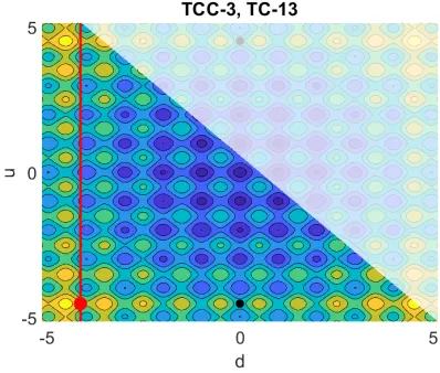
FunctionsT CC-3 andT CC-5, instead, depend on both design
dand uncertainu. Also they force the solution to move from the unconstrained one in TABLE II to TABLE IV.
TABLE III
TEST CASES FOR THE CONSTRAINT FUNCTIONSC
name constraint functionT CC
TCC-1 C(d) =
Pn−1
i=1
q
A2
1−(d1−x0)2+B1,i−di+1 ifd1≥x0 - R
Pn−1 i=1
q
A2
1−(d1−x0+ 2A1)2+B1,i−di+1 else TCC-2 C(d) =A2·n+P[d2i−A2·cos(2πdi)]−B2
TCC-3 C(d, u) =PN i=1
max 0, di+ui−A7
TCC-4 C(d, u) =
(
1 if any|di−d∗i| ≤ν9 −1 else
TCC-5 C(d, u) =
(
−1 if|d−d∗| ≤C
A14(||d||+||u||) +PNi=1(d2i+u2i−A14cos(2πdi) + cos(2πui)−5 else
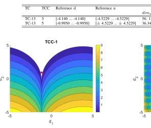
TABLE IV
REFERENCE SOLUTIONS FOR THE TEST CASES IN TABLEI,WITH CONSTRAINTS THAT MOVE THE MIN-MAX
TC TCC Reference d Reference u f min-max
[image:5.612.104.508.71.213.2]dimd,u= 1 dimd,u= 2 dimd,u= 3 TC-13 3 [-4.140 ... -4.140] [-4.5229 ... -4.5229] 56. 118 117.2373 178.3559 TC-13 5 [-0.9950 ... -0.9950] [±4.5229 ...±4.5229] 36.3482 77.6965 119.0447
Fig. 2. Contour ofT CC-1 where the white area is the feasible domain and min-max solution (red point) forp6,1.
coefficientsAi,Bi andCi, as written in TABLE III, in order to be applied to the differentT Cs in TABLE II. T CC-1 and T CC-2 requires at least 2 elements in the design vector and then they are applied to test functions from T C-1 to T C-6, T C-11 andT C-12.
The optimiser used for both optimisation and restoration loops is M P-AIDEA [28]. M P-AIDEA has been used with one and three populations. Parameters have been set as follows: the number of agents for each population is equal to the number of variables (dimdin the outer loop anddimuin
[image:5.612.67.363.244.495.2]the inner loop); the maximum number of local restart is iun = 20 for one population and it is adaptive for 3 populations; the crossover probability, CR, and the differential weight,F are self adapted; the size of the convergence box is ρ= 0.25;
Fig. 3. Contour ofT CC-2 where the white area is the feasible domain and min-max solution (red point) forp1,2
the distance from the cluster centres for the global restart is δglobal = 0.1 and the dimension of the bubble for the local restart, if not adapted, is δlocal = 0.1.
B. Test Results
The convergence of M acM inM ax has been tested with different values of Nmax
f eval that results from the combination of the number of function evaluation in the inner loop Nin f and in the outer loopNout
f . Different tolerancestolf andtolu, also, have been considered. TABLE IX reports some results with 1 and 3 populations. Fig.5 shows an example of success rate for an increasing number of function calls, for the case of problemp6,1. In the figure, for eachNf evalmax the bestSRs - over all combinations ofNin
f andN out
Fig. 4. Contour ofT CC-5 where the white area is the feasible domain. The min-max solution ofT C-13 withoutT CC-5 is the black point while the red point is the feasible solution forp13,5
Fig. 5. Success Rates for problemp6,1 (T C-6 andT CC-1) with different Nmax
f eval, evaluated from the three tolerances described in Algorithm 2 -tolf, tolc andtolu - independently. In particular,SRf has been evaluated with three values oftolf.
In TABLES V, VI, VII, VIII, IX, X, XI and XII it is shown that the higher both Nin
f andNfout are, the more accurate are the maxima and minima evaluated at each optimisation-restoration loop but the overall cost of the min-max algorithms increases accordingly. If the total cost is kept fixed an increase of Nin f andNout
f does not necessarily lead to an improvement of the solution. In Fig. 7, for example, for Nfin=Nfout = 200 the algorithm has a poor success rate for all function evaluations. When the number of function evaluations of the inner and outer levels is increased to 300, the success rate improves rather quickly. When the number of function evaluations of the inner and outer loops is increased even further, the success rate progressively decreases, for a constant number of total function evaluations. By setting Nin
f too small, the convergence is not guaranteed even with a very highNout
f and
usually the solution is underestimated. On the other hand for a lowNout
f , the algorithm stagnates at different local minima - if T C-i and/or T CC-j are multimodal - and it does not converge, or converges slowly, even with an highNfin.
IV. CONCLUSION
[image:6.612.321.552.339.553.2]In this paper we have presented a novel method for the solution of the constrained min-max problem. The algorithm was extensively tested on a new benchmark of objective and constraint functions with a variety of features that can be encountered in real-life applications. Results show that the algorithm we proposed is generally successful at identifying the constrained min-max solution with a limited number of calls to objective functions and constraints. The unconstrained version of the algorithm proposed in this paper was already proven to be efficient and reliable compared to existing evo-lutionary and non-evoevo-lutionary algorithms. We argue that also this constrained version is equally reliable and efficient given the good success rate displayed on most of the test functions. Future developments will include the use of surrogate models to further reduce the calls to objective and constraints functions.
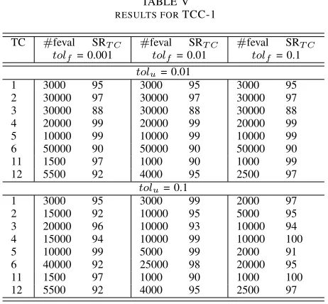
TABLE V RESULTS FORTCC-1
TC #feval SRT C #feval SRT C #feval SRT C tolf = 0.001 tolf = 0.01 tolf = 0.1
tolu= 0.01
1 3000 95 3000 95 3000 95
2 30000 97 30000 97 30000 97
3 30000 88 30000 88 30000 88
4 20000 99 20000 99 20000 99
5 10000 99 10000 99 10000 99
6 50000 90 50000 90 50000 90
11 1500 97 1000 90 1000 99
12 5500 92 4000 95 2500 97
tolu= 0.1
1 3000 95 3000 99 2000 97
2 15000 92 10000 95 5000 95
3 20000 96 10000 93 10000 94
4 15000 94 10000 99 10000 100
5 10000 99 5000 99 2000 91
6 40000 92 25000 98 20000 95
11 1500 97 1000 90 1000 100
12 5500 92 4000 95 2500 97
TABLE VI
RESULTS FORTCC-1ANDTC-13
dim #feval SRT C #feval SRT C #feval SRT C tolf = 0.001 tolf = 0.01 tolf = 0.1
tolu= 0.01
1 5000 100 5000 100 1000 94
2 20000 94 20000 95 15000 90
3
tolu= 0.1
1 5000 100 5000 100 5000 100
2 20000 94 20000 95 15000 90
[image:6.612.319.552.429.698.2]TABLE VII RESULTS FORTCC-2
TC #feval SRT C #feval SRT C #feval SRT C tolf = 0.001 tolf = 0.01 tolf = 0.1
tolu= 0.01
1 15000 95 15000 96 15000 96
2 30000 98 30000 98 30000 98
3 90000 71 90000 71 90000 71
4 30000 94 30000 94 30000 94
5 30000 100 30000 100 30000 100
6 100000 13 100000 13 100000 13
11 2500 94 2500 97 1500 91
12 7000 78 7000 87 7000 89
tolu= 0.1
1 15000 95 10000 100 5000 91
2 20000 91 20000 98 10000 95
3 90000 89 50000 98 40000 93
4 30000 98 15000 98 10000 98
5 30000 100 10000 91 10000 98
6 100000 23 100000 74 90000 90
11 2500 94 2500 97 1500 91
12 7000 78 7000 87 6000 90
TABLE VIII
RESULTS FORTCC-2ANDTC-13
dim #feval SRT C #feval SRT C #feval SRT C tolf = 0.001 tolf = 0.01 tolf = 0.1
tolu= 0.01
1 1000 99 1000 99 1000 100
2 10000 95 10000 96 10000 96
3 90000 92 90000 93 60000 90
tolu= 0.1
1 1000 99 1000 99 1000 100
2 10000 95 10000 96 10000 96
[image:7.612.321.551.314.580.2]3 90000 92 90000 93 60000 90
TABLE IX
RESULTS FORTCC-3ANDTC-13
dim #feval SRT C #feval SRT C #feval SRT C tolf = 0.001 tolf = 0.01 tolf = 0.1
1 population MP-AIDEA tolu= 0.01
1 30000 68 5000 70 20000 71
2 80000 30 50000 73 70000 76
3 70000 3 90000 24 80000 36
tolu= 0.1
1 30000 68 5000 70 20000 71
2 80000 30 50000 73 70000 76
3 100000 3 90000 24 80000 36
3 population MP-AIDEA tolu= 0.01
1 5000 94 5000 96 5000 96
2 100000 38 100000 86 90000 90
3 80000 3 80000 11 80000 32
tolu= 0.1
1 5000 94 5000 96 5000 96
2 100000 38 100000 86 90000 90
3 80000 3 80000 11 80000 32
REFERENCES
[1] H. G. Beyer and B. Sendhoff, ”Robust optimisation - A comprehensive survey”, Comp. Methods Appl. Mech. Emgrg. 196 (2007) 3190-3218. [2] B. Rustem, ”Algorithms for Nonlinear Programming and Multiple
Objective Decisions”, Wiley, Chichester (1998).
Fig. 6. problemp13,3withdimd=dimu= 1. The contour corresponds to T C-13 while the area in transparency is the set of the unfeasible configura-tions (d,u). The black points correspond to the solution of the unconstrained problem. The solution is feasible for any realisation ofuifd∈[-5.14 5.14]. The red point is the solution for the constrained min-max problem.
TABLE X
RESULTS FORTCC-4WITHν= 0.01
TC #feval SRT C #feval SRT C #feval SRT C tolf = 0.001 tolf = 0.01 tolf = 0.1
tolu= 0.01
1 10000 95 10000 95 10000 95
2 30000 95 30000 95 30000 95
3 50000 99 50000 99 50000 99
4 30000 100 30000 100 30000 100
5 10000 96 10000 96 10000 96
6 50000 96 50000 96 50000 96
7 1000 100 1000 100 1000 100
8 4500 76 4500 76 4500 76
9 6000 19 6000 19 6000 19
10 5000 53 5000 53 5000 53
11 5500 88 6000 93 5500 96
12 4000 91 3500 92 3000 94
tolu= 0.1
1 10000 95 10000 95 10000 95
2 30000 95 30000 95 30000 95
3 30000 98 30000 99 30000 99
4 30000 100 30000 100 30000 100
5 10000 96 10000 96 10000 96
6 40000 96 40000 96 40000 96
7 1000 100 1000 100 1000 100
8 4500 76 4500 76 4500 76
9 6000 19 6000 19 6000 19
10 5000 54 5000 54 5000 54
11 5500 88 6000 93 5500 96
12 4000 91 3500 92 3000 94
[3] R. W. Chaney, ”A method of centers algorithm for certain minimax problems”, Volume 22, Issue 1, pp 202-226 (1982).
[4] R. Klessig and E. Polak, ”A method of feasible directions using function approximations with applications to min max problems”, Journal of Mathematical Analysis and Applications,vol: 41 (3) pp: 583-602 (1973). [5] V. Panin, Linearisation method for continuous minmax problem”,
Springer, Volume 17, Issue 2, pp 239243, March 1981.
[6] Y. M. Danilin, V. M. Panin, and B. N. Pshenichnyi, ”On the Shannon Capacity of a graph”, Notes Control and Information Sci, vol: 23 (30) pp: 51-57 (1982).
[7] VF Damyanov, VN Malozemov (1974) Wiley, New York.
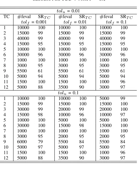
[image:7.612.57.288.443.662.2]TABLE XI
RESULTS FORTCC-4WITHν= 0.1
tolu= 0.01
TC #feval SRT C #feval SRT C #feval SRT C tolf = 0.001 tolf = 0.01 tolf = 0.1
1 10000 100 10000 100 10000 100
2 15000 99 15000 99 15000 99
3 40000 99 40000 99 40000 99
4 15000 95 15000 95 15000 95
5 10000 100 10000 100 10000 100
6 30000 96 30000 96 30000 96
7 1000 100 1000 100 1000 100
8 3000 95 3000 95 3000 95
9 5500 61 5500 61 5500 61
10 5000 94 5000 94 5000 94
11 1500 100 1500 100 1000 96
12 5000 88 3500 90 3000 97
tolu= 0.1
1 10000 100 10000 100 5000 99
2 15000 99 15000 100 15000 100
3 30000 99 20000 99 20000 100
4 15000 98 10000 96 10000 97
5 10000 100 5000 100 5000 100
6 30000 100 15000 98 15000 100
7 1000 100 1000 100 1000 100
8 3000 95 2000 95 2000 95
9 6000 79 5500 84 5500 84
10 5000 97 5000 97 5000 97
11 1500 100 1500 100 1000 96
[image:8.612.51.290.74.690.2]12 5000 88 3500 90 3000 97
TABLE XII
RESULTS FORTCC-5ANDTC-13
dim #feval SRT C #feval SRT C #feval SRT C tolf = 0.001 tolf = 0.01 tolf = 0.1
tolu= 0.01
1 10000 100 10000 100 10000 100
2 70000 94 50000 90 50000 91
3 90000 49 90000 49 90000 49
tolu= 0.1
1 10000 100 10000 100 10000 100
2 70000 94 50000 90 50000 91
3 90000 49 90000 49 90000 49
[9] J. S.H. Wang and W. W.M. Dai, ”Transformation of min-max optimiza-tion to least-square estimaoptimiza-tion and applicaoptimiza-tion to interconnect design optimization,” Proceedings of ICCD ’95 International Conference on Computer Design. VLSI in Computers and Processors, Austin, TX, USA, 1995, pp. 664-670.
[10] B. Lu, Y. Cao, M. Yuan and J. Zhou, ”Reference variable methods of solving minmax optimization problems”, Journal of Global Optimiza-tion, 2008 vol: 42 (1) pp: 1-21.
[11] M. A. Sainz, P. Herrero, J. Armengol and J. Vehi, ”Continuous minimax optimization using modal intervals”, J. Math. Anal. Appl, 2008 vol: 339 pp: 18-30.
[12] Y. Feng, L. Hongwei, Z. Shuisheng and L. Sanyang, ”A smoothing trust-region Newton-CG methodfor minimax problem”, Applied Mathematics and Computation, 2008 vol: 199 (2) pp: 581-589.
[13] P. Parpas and B. Rustem, ”An Algorithm for the Global Optimization of a Class of ContinuousMinimax Problems”, Journal of Optimization Theory and Applications, 2009 vol: 141 (2) pp:461-473.
[14] T. M. Cavalier, W. A. Conner, E. del Castillo and S. I. Brown, ”A heuristic algorithm for minimax sensor location in the plane”, European Journal of Operational Research , vol. 183,no. 1, pp. 4255, 2007. [15] D. Ahr and G. Reinelt, ”A tabu search algorithm for the minmax
k-chinese postman problem”, Computers and Operations Research , vol. 33, no. 12, pp. 3403-3422, December 2006.
[16] A.M. Cramer, S.D. Sudhoff and E.L. Zivi, ”Evolutionary algorithms
Fig. 7. Convergence of the Success Rate for problemp6,4with an increasing number ofNin
f =Nfout.
for minimax problems in robust design”. IEEE Trans. Evolut. Comput. 13(2), 444-453 (2009)
[17] R.I. Lung and D. Dumitrescu, ”A new evolutionary approach to minimax problems”. In: Proceedings of the 2011 IEEE Congress on Evolutionary Computation, New Orleans, USA, pp. 1902-1905 (2011)
[18] A. Sinha, Z. Lu, K. Deb and P. Malo, ”Bilevel Optimization based on Iterative Approximation of Multiple Mappings”.
[19] A. Sinha, P. Malo, K. Deb, ”A Review on Bilevel Optimization: From Classical to Evolutionary Approaches and Applications”.
[20] M. Vasile, ”On the solution of min-max problems in robust optimisa-tion”. In: The EVOLVE 2014 International Conference, A Bridge be-tween Probability, Set Oriented Numerics, and Evolutionary Computing, 2014-07-01 - 2014-07-04, Jian-Guo Hotel (2014).
[21] K. Shimizu and E. Aiyoshi, ”Necessary conditions for min-max prob-lems and algorithms by a relaxation procedure”, IEEE Trans. Autom. Control25 (1), 6266 (1980).
[22] K. Shimizu, Y. Ishizuka and J.F. Bard, ”Non-differentiable and Two-level Mathematical Programming”, Springer US (1997)
[23] J. Marzat, E. Walter and H. P. Lahanier, ”Worst-case global optimisation of black-box functions through Kriging and relaxation”, Journal of Global Optimization, 2013.
[24] G. Filippi, M. Marchi, M. Vasile and P. Vercesi, ”Evidence-Based Robust Optimisation of Space Systems with Evidence Network Models”, In 2018 IEEE Congress on Evolutionary Computation (CEC) (pp. 18). [25] B. Rustem and M. Howe, ”Algorithms for Worst-Case Design and
Ap-plications to Risk Management”, Princeton University Press, Princeton, NJ (2002).
[26] A. Zhou, Q. Zhang, ”A surrogate-assisted evolutionary algorithm for minimax optimization”. IEEE Congress on Evolutionary Computation, Barcelona, Spain, pp. 17 (2010)
[27] M. Vasile, E. Minisci and M. Locatelli, ”An Inflationary Differential Evolution Algorithm for Space Trajectory Optimization”, IEEE Trans-action on Evolutionary Computation, vol. 15, no. 2, April 2011. [28] M. Di Carlo, M. Vasile and E. Minisci, ”Multi-population adaptive