City, University of London Institutional Repository
Citation:
Andrienko, N., Andrienko, G. and Rinzivillo, S. (2016). Leveraging spatial
abstraction in traffic analysis and forecasting with visual analytics. Information Systems, 57,
pp. 172-194. doi: 10.1016/j.is.2015.08.007
This is the accepted version of the paper.
This version of the publication may differ from the final published
version.
Permanent repository link:
http://openaccess.city.ac.uk/13599/
Link to published version:
http://dx.doi.org/10.1016/j.is.2015.08.007
Copyright and reuse: City Research Online aims to make research
outputs of City, University of London available to a wider audience.
Copyright and Moral Rights remain with the author(s) and/or copyright
holders. URLs from City Research Online may be freely distributed and
linked to.
Leveraging Spatial Abstraction in Traffic Analysis and Forecasting with Visual
Analytics
Natalia Andrienko1, Gennady Andrienko1, and Salvatore Rinzivillo2
Abstract— A spatially abstracted transportation network is a graph where nodes are territory compartments (areas in geographic space) and edges, or links, are abstract constructs, each link representing all possible paths between two neighboring areas. By applying visual analytics techniques to vehicle traffic data from different territories, we discovered that the traffic intensity (a.k.a. traffic flow or traffic flux) and the mean velocity are interrelated in a spatially abstracted transportation network in the same way as at the level of street segments. Moreover, these relationships are consistent across different levels of spatial abstraction of a physical transportation network. Graphical representations of the flux-velocity interdependencies for abstracted links have the same shape as the fundamental diagram of traffic flow through a physical street segment, which is known in transportation science. This key finding substantiates our approach to traffic analysis, forecasting, and simulation leveraging spatial abstraction.
We propose a framework in which visual analytics supports three high-level tasks, assess, forecast, and develop options, in application to vehicle traffic. These tasks can be carried out in a coherent workflow, where each next task uses the results of the previous one(s). At the ‘assess’ stage, vehicle trajectories are used to build a spatially abstracted transportation network and compute the traffic intensities and mean velocities on the abstracted links by time intervals. The interdependencies between the two characteristics of the links are extracted and represented by formal models, which enable the second step of the workflow, ‘forecast’, involving simulation of vehicle movements under various conditions. The previously derived models allow not only prediction of normal traffic flows conforming to the regular daily and weekly patterns but also simulation of traffic in extraordinary cases, such as road closures, major public events, or mass evacuation due to a disaster. Interactive visual tools support preparation of simulations and analysis of their results. When the simulation forecasts problematic situations, such as major congestions and delays, the analyst proceeds to the step ‘develop options’ for trying various actions aimed at situation improvement and investigating their consequences. Action execution can be imitated by interactively modifying the input of the simulation model. Specific techniques support comparisons between results of simulating different “what if” scenarios.
1 Natalia Andrienko and Gennady Andrienko are with Fraunhofer Institute IAIS, Schloss Birlinghoven, 53757
Sankt Augustin, Germany and City University London, UK. E-mail: {natalia|gennady}[email protected].
2 Salvatore Rinzivillo is with the Knowledge Discovery Laboratory, Istituto di Scienza e Tecnologie
dell'Informazione, Area della Ricerca CNR, via G. Moruzzi 1, 56124 Pisa, Italy. E-mail: [email protected].
1 INTRODUCTION
Data concerning vehicle traffic can be nowadays collected in unprecedented amounts owing to the advances in the sensing technologies. These data offer new opportunities for improving the understanding of traffic properties and enhancing the accuracy of models forecasting traffic situations and their evolution. However, the potential of real traffic data remains largely underexploited. By means of visual analytics methods, we performed a systematic focused study to investigate the potential opportunities offered by traffic data. We found that historical traffic data can not only enable understanding of spatio-temporal patterns of traffic flows and interdependencies between their key characteristics (speed and volume), but they can also be used for building mathematical and computational models capable of forecasting traffic situations and their developments under various conditions. This finding is a result of an evolutionary process of design, implementation, and application of a range of visual analytics methods focusing on movement analysis [2].
routes and investigate their impacts on the traffic situation development, including comparative analysis of various “what if” scenarios.
The contribution of our research is twofold. First, we comprehensively explored the potential opportunities offered by traffic data and demonstrated the possibilities of using them not only for analysis of past situations but also for efficient forecasting and “what if” analysis. Second, we developed an integrated visual analytics framework for traffic analysis, modeling, and forecasting, which supports a seamless workflow involving different analytical tasks. Specifically, our framework supports three major types of analytical tasks ([61], p. 35): assess (i.e., understand the piece of reality represented by available data), forecast (i.e., estimate the properties or behavior of the piece of reality beyond the part represented in the data), and develop options (i.e., find actions that can change the properties or behavior of the piece of reality in a desired way).
Although the three types of tasks can be treated as independent activities [61], it is obvious that these can also be stages of a single analytical process, in which ‘forecast’ builds on results of ‘assess’ and, in turn, enables ‘develop options’. So far, it has not been usual for visual analytics researchers to strive at supporting the whole process comprising all three types of tasks. Our work thus makes a contribution to visual analytics research not only by proposing a set of application-oriented techniques but also by demonstrating a way to support such a process. Although the immediate results of our work are specific to traffic analysis, the experience we gained and the framework incorporating it can be generalized and used by other researchers. The flow chart in Fig. 1 schematically represents a generalized view of an analytical process and exhibits the generic subtasks that need to be supported by visual analytics methods.
[ Fig. 1. Three types of visual analytics tasks as stages of a single analytical process. ]
At the first stage (‘assess’), analysts study available data to understand the phenomena reflected in the data. The understanding gained by the analysts can be seen as a mental model of the phenomenon. It is beneficial for the further analysis to externalize this model, preferably, in a form permitting computer processing. The analysts may derive several models representing different aspects of the phenomenon. Each model must be assessed and validated. At the second stage (‘forecast’), the models are used to forecast events and developments that can occur under some conditions of interest. The analysts assess the resulting forecast to see the “capabilities, threats, vulnerabilities, and opportunities” ([61], p. 35) and understand whether the predicted situation or process requires intervention. If so, the analysts proceed to the third stage (‘develop options’), in which they choose actions for improving the situation/process and perform the task ‘forecast’ to see and assess the effects of the chosen actions. The analysts also need to compare predicted results of different possible interventions.
This general scheme can be instantiated for various applications. The generic subtasks need to be specialized for a given application, thereby setting specific objectives for design and development of visual analytics tools.
In this paper, we present an instantiation of the general scheme for vehicle traffic analysis and include a special discussion of possible ways to validate traffic forecasting models using real data. Due to the novelty of our approach to traffic modeling and simulation, we find it reasonable to begin with presenting evidence of the existence and uniformity of the fundamental traffic relationships in spatially abstracted transportation networks at different spatial scales (section 2). After this, we give an overview of related works (section 3) and then describe our framework in section 4, dealing consecutively with the tasks ‘assess’ (analysis and modelling of historical traffic data; subsection 4.1), ‘forecast’ (traffic simulation; subsection 4.2), and ‘develop options’ (forecasting and comparison of consequences of possible traffic regulation actions; subsection 4.3). Section 5 presents our approach to the evaluation and validation of models built according to our framework, and section 6 contains a concluding discussion. Additionally, the web page http://geoanalytics.net/and/is2015/ contains full color versions of all figures, a video demonstrating the analytical process, and a slide presentation.
2 LEVERAGING SPATIAL ABSTRACTION: APPROACH SUBSTANTIATION
2.1 Creation of a spatially abstracted transportation network
After obtaining a division of the underlying territory into cells, the trajectories are transformed into flows (aggregate movements) between the cells. For each ordered pair of cells Ci and Cj, a flow is an aggregate of individual moves from Ci to Cj, where a move is a pair of consecutive points from one trajectory such that the first point is inside Ci and the second point is inside Cj. Two cells Ci and Cj are said to be linked if there is at least one move from Ci to Cj in the dataset. An ordered pair of linked cells is called a link. Note that such a link is not a physically existing entity but an abstract construct. A combination of a set of cells C and a set of links L is considered as an abstract transportation network. In mathematical terms, <C, L> is a graph where C is the set of nodes and L is the set of edges.
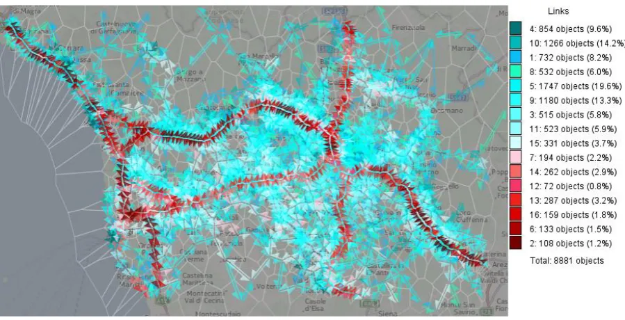
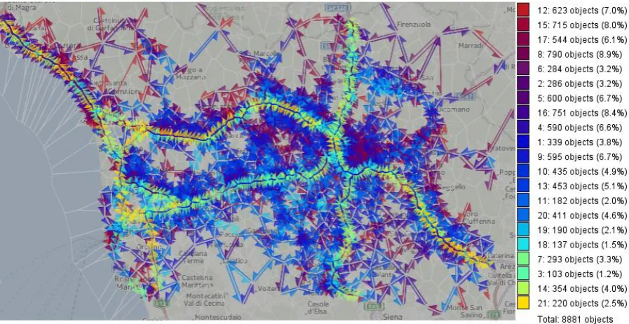
As an illustration, Figure 2 shows a map with a spatially abstracted transportation network of Milan (Italy) reconstructed from GPS tracks of 17,241 cars collected over a period of one week from Sunday, April 1, to Saturday, April 7, 2007 (data source: Octo Telematics SpA; http://www.octotelematics.com). The territory of Milan is divided into cells with approximate radii of 1 km. The cell boundaries are shown as grey lines. For showing the abstract links, we apply the flow map technique [43][59], which represents flows by straight or curved linear symbols. The widths and/or colors of the lines may encode characteristics of the flows. Movement directions can be shown by arrows; however, when it is necessary to represent opposite flows between the same places, cartographers and visualization designers use half-arrows [62] or curved lines with the curvature increasing towards the flow destination [67]. These two possibilities are illustrated in enlarged map fragments on the right of Fig. 2. In the whole map, curved lines are used. For improving the map legibility, the flow symbols are differently colored. The meaning of the colors will be explained later.
[ Fig. 2. A spatially abstracted transportation network of Milan (Italy) with cell radii 1km. ]
2.2 Spatio-temporal aggregation of movement data
For the further analysis, the trajectories are aggregated into flows by time intervals. For each link (Ci, Cj) and each time interval Tk, the corresponding flow is an aggregate of all moves from Ci to Cj that ended within the interval Tk and started within either Tk or Tk-1. The flow is characterized by the number of moves and the mean speed (velocity) of the movement. The number of moves (traffic volume) per time interval is called traffic intensity (in some literature, the terms traffic flow or flux are used). The mean speed is computed as follows. For each object that moved from cell Ci to cell Cj, two trajectory points that are the closest to the centers of these cells are selected. Dividing the length of the path between the selected points by the time difference between them gives the mean speed of this object. The overall mean speed on the link (Ci, Cj) in a time interval Tk is computed as the mean of the mean speeds of all objects that moved from Ci to Cj during Tk. Hence, the aggregation of the trajectories into flows by time intervals produces two sets of time series associated the links: traffic intensities and mean speeds.
In our example in Fig. 2, we applied partition-based clustering (k-means) to the time series of flow characteristics, i.e., the links have been clustered by the similarity of the associated time series of the flow intensities and mean speeds. Colors have been assigned to the resulting clusters in such a way that similar colors correspond to similar clusters [7]. These colors have been used to paint the flow symbols on the map. The color legend on the left of Fig. 2 shows the colors assigned to the clusters and the cluster sizes, i.e., the number of links in each cluster and the percentage of the total number of links.
2.3 Interdependencies between traffic intensities and mean speeds
To study and quantify the relationships between the traffic intensities and mean speeds on the links, the data are transformed in the following way. Let A and B be two time-dependent attributes associated with the same object (in particular, link) and defined for the same time steps. In particular, A may stand for the traffic intensity and B for the mean speed, or vice versa.
1. Divide the value range of attribute A into intervals. 2. For each value interval of A:
a. Find all time steps in which the values of A fit in this interval. b. Collect all values of B occurring in these time steps.
c. From the collected values of B, compute summary statistics: quartiles, 9th decile, and maximum.
similar to a time series except that the steps are based not on time but on values of attribute A. We call such sequences dependency series since they express the dependency between attributes A and B. Attribute A is treated as the independent variable and B as the dependent variable.
To study and model the interdependencies between the mean speed and the traffic intensity, we perform two transformations. First, we treat the traffic intensity as the independent variable and derive a family of attributes expressing the dependency of the mean speed on the traffic intensity. Second, we treat the mean speed as the independent variable and derive a family of attributes expressing the dependency of the traffic intensity on the mean speed. Dependency series may be derived using either the absolute or relative traffic intensities, the latter being computed as the ratios or percentages of the absolute intensities to the maximal intensities attained on the same links.
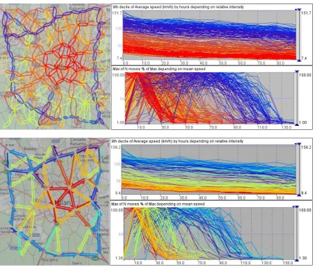
[ Fig. 3. The graphs represent the interdependencies between the traffic intensity and mean speed for the link of the abstracted transportation network of Milan shown in Fig. 2. ]
The dependencies we have derived for the abstracted transportation network of Milan shown in Fig.2 are graphically represented in Fig.3. The lines in the graphs correspond to the links of the network and are colored according to the cluster membership of the links using the same colors as in Fig.2. The graph on the left represents the dependencies of the mean speed on the relative traffic intensity in percent to the maximum. The horizontal axis corresponds to the traffic intensity (N moves % of max) and the vertical axis to the 9th decile of the mean speed. We have taken the 9th decile because this statistical measure is less sensitive to outliers as the maximum. Outliers among the values of the mean speed often occur in time intervals of low traffic intensity, when a single or only a few vehicles traverse a link. The graph on the right represents the dependencies of the relative traffic intensity on the mean speed. The horizontal axis corresponds to the mean speed and the vertical axis to the maximal traffic intensity.
On the left of Fig.3, the shapes of the lines show that the mean speed decreases with increasing traffic intensity. On the right, the lines have the shape of a bell or symbol ‘’. This shape can be interpreted as follows. When vehicles move with a low mean speed, only a small number of vehicles can traverse a link in a time unit. When the mean speed increases, the number of vehicles also increases, but only till the point when a certain “optimal” value of the mean speed is reached. After this point, movement with higher mean speeds is only possible when the traffic load decreases. These observations conform to our commonsense knowledge and experiences concerning the behavior of the vehicle traffic on roads but refer to an abstracted rather than physical transportation network.
[ Fig. 4. The dependencies between the traffic intensity and mean speed can be represented by polynomial regression models. ]
Figure 4 demonstrates how the dependencies the traffic intensity and mean speed can be represented by formal models, such as polynomial regression (other kinds of curves can be fitted as well). The modeling is done for clusters of links rather than for each individual link, to avoid over-fitting and reduce the impact of local outliers and fluctuations. The fitted curves capture the character of the dependencies. These curves have the same shape as the fundamental diagram of traffic flow describing the relationship between the flow velocity and traffic flux (i.e., intensity) [27] (see also http://en.wikipedia.org/wiki/Fundamental_diagram_of_traffic_flow). The fundamental diagram refers to links of a physical transportation network, i.e., to street segments. The exact parameters of the curves depend on the street properties, such as the width, number of lanes, and speed limit. We see that the same relationships as in a physical network exist also in a spatially abstracted network. Moreover, we have found that the relationships conforming to the fundamental traffic diagram exist on different levels of spatial abstraction, as illustrated in Fig. 5. The parameters of the curves depend on the properties of the abstracted links. As each abstracted link stands for a group of physical links, its properties incorporate and summarize the properties of these physical links.
[ Fig. 5. The maps show spatially abstracted transportation networks of Milan with cell radii 2km (top) and 4 km (bottom). The graphs to the right of each map represent the dependencies between the relative traffic intensities and the mean speeds on the network links. ]
2.4 Advantages and limitations of spatial abstraction
The fundamental relationships between the traffic flow characteristics represented by the conventional traffic flow diagram are commonly used for traffic flow prediction and simulation, which is usually done for a physical street network. The existence of the same relationships at higher levels of spatial abstraction makes it possible to do modeling, prediction, and simulation also at higher spatial scales in cases when fine details are not necessary. Spatial abstraction of a street network offers the following advantages:
• The number of nodes and links in an abstracted network can be much smaller than in the underlying physical network. Hence, much less time and effort is needed for model building and calibration, and also simulations can be carried out much faster compared to the current practices. This enables, in particular, rapid approximate predictions and assessments in emergency situations, when time is very limited.
• Spatial abstraction compensates for the sparseness of real data on streets with low traffic. There may be not enough trajectory points on a given street segment for reconstructing the dependency between the mean speed and traffic intensity, but aggregation of several physical links into one abstract link alleviates the problem.
• As mentioned earlier and will be shown by example further in the paper, it is possible to build an abstract network in which the level of spatial abstraction varies across a territory according to the variation of the data density. In areas with high traffic, abstracted links may very closely approximate physical links (i.e., street segments), whereas areas with low traffic can be represented by large cells. Hence, it is possible to have different levels of detail in traffic simulations and prediction in areas with high and low traffic, when fine details in low traffic areas are not important.
• Spatial abstraction may also serve as a tool for protecting locational data privacy [50].
There are certain limitations for applying spatial abstraction. Obviously, it is not applicable to problems requiring detailed analysis and modelling of traffic at the level of street segments and junctions. However, even when problem settings permit abstraction, the spatial scale (i.e., the cell sizes) cannot be unlimitedly increased without distorting and eventually destroying the shapes of the curves representing the relationships between the traffic fluxes and velocities. Generally, increasing the spatial scale increases the amount of noise (i.e., oscillations) within the curves. The overall shapes of the curves remain discernible up to a certain abstraction level, at which the oscillations become too high. Our experiments show that the upper limit for the cell sizes may depend on the number and diversity of the existing physical links between the cells. Thus, for Milan and the urban areas of Tuscany, increasing the cell radius beyond 4 km distorts the curves too much, whereas much larger cells can be used for the rural areas of Tuscany. Hence, there is no uniform upper limit to the level of spatial abstraction that would be valid everywhere. An appropriate level for a given territory and available data can be determined empirically with the use of visual analytics techniques.
One reservation needs to be made concerning the reconstruction of the fundamental relationships between the traffic flow characteristics from real vehicle trajectories. It is typical that available trajectories cover only a sample of vehicles that move within a network and not the entire population. Hence, the traffic intensities computed from these trajectories need to be appropriately scaled, to approximate the real intensities. This reservation is not specific to spatially abstracted networks but also applies to detailed street networks. Appropriate scaling parameters (or even scaling functions capturing daily and weekly variations) can be obtained by comparing the vehicle counts computed from trajectory data with real traffic counts obtained from traffic sensors [54]. The issue of data scaling lies out of the scope of this paper.
3 RELATED WORKS
3.1 Visual Analytics Methods for Analysis of Movement Data
Analysis of movement data, including data concerning vehicle traffic, is one of the most important topics in many fields of research, including data mining [29], geographic information science [31], and visual analytics [6]. The majority of the existing works concentrate on (1) visualization and interactive exploration of spatial and temporal aspects of individual trajectories [39][63] and sets of trajectories [32][36], (2) analysis of movement attributes along trajectories [32][60][63][68], (3) detecting stops, interactions between trajectories, and other kinds of events [9][10], (4) aggregating movement data in space and time and visualization of resulting aggregates [23][65][66][67], and (5) revealing relationships between movement and the environment (context) [45].
Works of Sewall et al. [56][57] focus on the ‘forecast’ task in movement (specifically, vehicle traffic) analysis. They developed traffic simulation algorithms allowing generation of realistic 3D animations of simulated vehicle movements. However, the forecasting is not linked to previous analysis of real data and to following development of options.
3.2 Visual Analytics Support to Modeling and Simulation
Multiple works in visual analytics support building and assessment of models in other application domains. Much attention has been given to classification models [25][30][69], including decision trees [24]. A classifier may be built for assigning new objects to previously obtained clusters [3][26]. Visual analytics techniques also support derivation of linear trend models from multivariate data [32], regression models [51], and time series models [13][34]. Other works focus on supporting assessment of existing models, including classification [49], engineering simulation [47][48], and spatio-temporal models [21][46][55]. In particular, comparative assessments of results of multiple simulations are supported [47][48][64].
There are works on supporting the tasks ‘forecast’ and ‘develop options’ in planning pandemic response [1][46] and flood protection [55][64]. Pre-existing simulation models are used to provide forecasts. Interactive environments allow users to assess the forecasts, imitate implementation of response measures, observe the effects of these measures, and compare expected results of different measures. The system World Lines [64] represents multiple simulation runs in a tree-like view. Each simulation is shown as a branch. User’s interventions create new branches, which are executed in parallel with previously existing ones allowing the user to compare the consequences of different response measures. In RunWatchers [41], a response plan is created automatically using multiple parallel simulations, and then the system visualizes the generated decision tree and presents the resulting plan in the form of a visual storyboard representing the recommended sequence of actions and justifications for the decisions taken.
We are not aware of visual analytics works on supporting the whole workflow ‘assess’ – ‘forecast’ – ‘develop options’ as presented in the introduction.
3.3 Transportation Research
According to the level of detail in representing traffic, there exist macroscopic, mesoscopic, and microscopic traffic simulation models [57]. Macroscopic models (a.k.a. continuous or continuum models [56]) describe the traffic at a high level of aggregation as flow without considering individual vehicles. This is done using sets of differential equations, which are often defined based on analogies to physical phenomena, such as gas or fluid dynamics [44]. The cell transmission model [18][19] is a discretized variant of the macroscopic approach.
In microscopic models, traffic is described at the level of individual vehicles and their interactions with each other and with the road infrastructure. Two major classes are agent-based models [53] and cellular automata models [52]. Being quite resource-demanding, microscopic models have traditionally been used for local simulations in small areas, but the increased power of computers and parallel computing have enabled microscopic simulations for large networks. A disadvantage of microscopic models is large effort required for model preparation.
Mesoscopic models fill the gap between macroscopic and microscopic models by combining individual vehicle representation with aggregate representation of traffic dynamics [16]. Individual vehicles or packets of vehicles move through links of a transportation network according to general speed-density relationships defined in traffic flow theories [20][27] or derived from real data [35]. These relationships involve a number of parameters, which can be set differently for different link types [16].
Hybrid simulation models combine macroscopic or mesoscopic models with microscopic models [14][15]. Different model types are applied to different parts of a network. Thus, Sewall et al. [57] perform agent-based simulation of individual vehicles in regions of user’s interest while a faster macroscopic model is used in the remainder of the network. Our algorithm, which is presented in section 4.2.1, can be classified as a hybrid of mesoscopic and microscopic simulation methods: it simulates in detail only movements of additional vehicles while regular traffic flows are involved in the simulation in an aggregate form.
There are a number of commercial and open-source software packages for traffic simulations [38][42]. An open-source package SUMO [12] is used for preparing and performing micro- and macroscopic simulations. In our framework, however, we do not use any of these packages because the simulation models they include cannot be easily fed by the outputs of the ‘assess’ stage.
3.4. How this Work Extends the State of the Art
‘develop options’. While the task ‘forecast’ alone has been addressed by Sewall et al. [56][57], our work is the first to propose visual analytics support to all three tasks together in a common framework.
Moreover, in the visual analytics research as a whole, it is usual to address one of the tasks, and only a few works address two of them [1][46][55][64]. Our work gives a first example of how all three tasks can be supported as a single workflow. It also proposes a general scheme of this workflow, which can be used in developing comprehensive visual analytics support for other applications.
In the transportation research, a usual way to use real data is for setting parameters of pre-existing theory-based models. Another usual feature is performing traffic simulation at the level of detailed street network. Distinctive features of our approach are the use of spatial abstractions of physical transportation networks and derivation of models for traffic forecasting (simulation) directly from real historical data.
4 PRESENTATION OF THE FRAMEWORK
We have developed a visual analytics framework supporting the task workflow ‘assess’ – ‘forecast’ – ‘develop options’ in analysis of network-constrained movement in geographic space. The framework is applicable to aggregated movement data associated with nodes and links of a network, which may be a physical street network or a spatially abstracted network, as described in section 2. The data must include traffic intensities, that is, counts of objects that moved through the links by time intervals, and corresponding mean speeds of their movement. Ideally, the counts should represent the entire population of the objects that moved over the network, but the framework can also be applied to counts representing a large sample of objects (see the reservation at the end of section 2). The length and temporal resolution of the time series must be suitable for capturing the traffic variation related to the daily and weekly temporal cycles. This means that the length must be at least one week (more is better) and the resolution must be at most one hour (finer is better); a coarser temporal resolution may conceal important daily patterns, such as morning and evening rush hours.
In describing the framework, we use a running example of aggregated data from the area of Tuscany in Italy. The data were derived from about 3 million GPS tracks (i.e., sequences of position records, more than 52 million records in total) of 42,686 private cars collected during May 2011 by company Octo Telematics SpA (http://www.octotelematics.com). To protect the personal privacy of the car owners, access to the original data could not be provided, but we could obtain spatially and temporally aggregated data. For this purpose, the territory was divided into compartments (Voronoi cells) [2][5] based on a random sample of 90,000 position records. The sizes of the cells vary across the territory depending on the data density. The original data were aggregated by these cells and 744 hourly time intervals from May 1 to May 31, 2011.
4.1 Assess
The visual analytics support to the ‘assess’ task includes techniques for exploratory analysis of movement data and interactive tools for derivation of formal models representing the spatio-temporal variation of traffic flows and the relationships between the traffic intensities and mean speeds [2][7]. The process of model building is supported by an interactive visual interface illustrated in Fig. 4. It allows the user to choose a suitable method from a library of modeling methods, test different parameter settings and find appropriate ones, generate a model, evaluate its quality, and, when necessary, refine the model.
In our approach, models are built for clusters of links of a (spatially abstracted) transportation network rather than for individual links, to avoid over-fitting and reduce the impacts of noise and local outliers. The links are clustered according to the similarity of the associated time series (TS) of traffic intensities and mean speeds using a partition-based clustering algorithm, such as k-means, and interactive tools enabling visually supported progressive clustering [7]. We build three sets of models: (1) models of the temporal variation of the traffic intensity in each cluster, (2) models of the dependencies of the mean speeds on the traffic intensities, and (3) models of the dependencies of the traffic intensities on the mean speeds. For the model set (1), we apply the double exponential smoothing (Holt-Winters) method [36], which captures the periodic character of the temporal variation regarding the daily and weekly time cycles. For the model sets (2) and (3), we apply polynomial regression models, as demonstrated in Fig.4.
Each model by itself makes a common prediction for all cluster members, but this prediction is individually adjusted for each cluster member based on the statistics of the distribution of its original values [7].
shape (which means the same character of the dependency) and differ only in the level on the Y-axis, i.e., the speed values attained.
[ Fig. 6. A: The dependency series of the mean speed versus the traffic intensity have been clustered by similarity. B: The dependencies are represented by polynomial or linear regression models. ]
[ Fig. 7. The links in the flow map are colored according to the cluster membership of the dependencies of the mean speeds on the traffic intensities (Fig. 6). ]
Fig. 8 demonstrates the modeling of the opposite dependency: how the maximal number of vehicles that can pass through a link during one hour depends on the mean speed. As previously, the DS of the maximal traffic intensities depending on the mean speeds have been clustered by similarity. The graph Fig. 8A shows DS from three selected clusters (when all clusters are shown simultaneously, the display gets too cluttered and illegible). The map in Fig. 9 shows the spatial distribution of all link clusters. To capture the dependencies, we apply polynomial regression models with higher polynomial orders than for the previous set of models, since the line shapes are more complex. Fig. 8B graphically represents the dependency models built for all clusters.
[Fig. 8. A: Three selected clusters of dependency series of the traffic intensity depending on the mean speed. B: The dependency curves built for all clusters.]
[Fig. 9. The links are colored according to the cluster membership of the dependencies of the traffic intensities on the mean speeds.]
To summarize, the ‘assess’ stage of the traffic analysis workflow is supported by interactive tools for progressive clustering (allowing refinement of selected clusters), data visualization on maps and graphs, interactive visual interface to a modeling library, and techniques for model assessment by analyzing residuals [7]. The output of the ‘assess’ stage consists of three sets of models:
• TMF (Temporal Models of Flows): a set of models predicting for each link the regular number of moving vehicles (traffic intensity) in different time intervals;
• DMSL (Dependency Models of Speed on Load): a set of models predicting the mean speed of the movement through each link depending on the load, i.e., the number of vehicles that try to move;
• DMFS (Dependency Models of Flow on Speed): a set of models predicting the maximal number of vehicles that will be able to move through each link depending on the mean speed with which the vehicles can move.
Model descriptions are stored externally in XML files. Based on these descriptions, the models can be later restored and used for traffic forecasting.
4.2 Forecast
Assuming that TMF appropriately represents the daily and weekly variation of the usual traffic, this set of models can be directly used for forecasting the usual traffic in a time period that is not covered by the available data. This kind of forecasting is supported by a tool that allows the user to specify the time period for which the forecast needs to be done. The tool divides the period into time intervals of the same length as in the description of TMF and then applies the model set to each link and each time interval to forecast the expected traffic intensity.
DMSL and DMFS are used for simulating unusual extra traffic that appears in addition to the regular traffic. We do not use any of the existing traffic simulation tools for two main reasons: (1) high effort required for representing the network topology and link properties, and (2) absence of an easy way to feed the tool with the dependencies defined by DMSL and DMFS. To enable a seamless transition from ‘assess’ to ‘forecast’ and the use of simulation in interactive settings (for this purpose, it needs to be fast), we have developed our own traffic simulation algorithm that can directly utilize all three sets of models derived from real data. No effort for network encoding and parameter setting is required, which allows the user to proceed seamlessly from the task ‘assess’ to the task ‘forecast’. The algorithm is implemented within the software system V-Analytics, which is downloadable from http://geoanalytics.net/V-Analytics/ and may be used free of charge for research and educational purposes.
4.2.1 Traffic Simulation Algorithm
different parts of the network [14][15], while we use them for different parts of the traffic, regular and extraordinary. Our approach allows the user to study specifically the development of the extra traffic and its interactions with the regular traffic. Still, the method can also be used in a more traditional form. It can simulate the movement of an explicitly specified population of vehicles without involving any background traffic flows, that is, assuming that the given population includes all vehicles existing on the territory under study. For this task, the simulation method does not use TMF and uses only DMSL and DMFS.
The main idea is following: for each link, the method finds how many vehicles need to move through it in the current minute, determines the mean speed that is possible for this link load (using DMSL), then determines how many vehicles will actually be able to move through the link in this minute (using DMFS), and then promotes this number of vehicles to the end place of the link and suspends the remaining vehicles in the start place of the link. A formal description of the algorithm is given below.
The system of places and links is represented as a directed graph G = (P, L), where P is the set of places and L is the set of links. Each link has a collection of dynamic (time-variant) properties. Current properties of the links can be determined by querying the models TMF, DMSL, and DMFS:
• TMF(l, t) gives the expected number of regular vehicles traversing link l at time t; • DMSL(l, n) gives the expected mean speed of n vehicles moving on link l;
• DMFS(l, s) gives the maximal number of vehicles able to move on link l with mean speed s.
The input of the simulation procedure includes the graph G, the models, and a population of additional vehicles V, where each vehicle has been assigned an origin node (place), a destination node, a route, i.e., a path through the graph from the origin to the destination, and a time moment when the vehicle can start the movement.
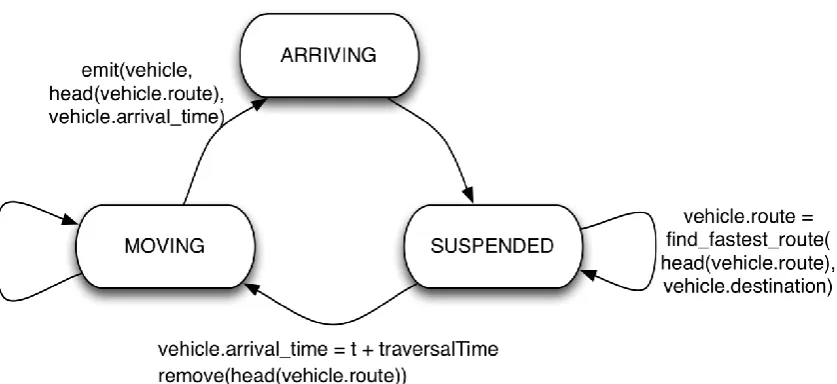
At each time instant t, a vehicle can be in one of the following states (Fig. 10):
• SUSPENDED: the vehicle is located in a node and is waiting to move towards the next node in its planned route;
• MOVING: the vehicle is moving on a link to reach the next node of its planned route; • ARRIVING: the vehicle arrives at one of the nodes of its planned route.
[Fig. 10. The possible states of vehicles and transitions between the states in the course of the simulation.]
If the current conditions allow a suspended vehicle to move, it can pass to the status MOVING; otherwise, it remains in the SUSPENDED status. When a vehicle changes the status to MOVING, it is assigned an expected time of arrival to the next node; the current node, in which the vehicle has been till this moment, is removed from the route of this vehicle. The vehicle will remain in the MOVING status until the simulation time reaches the assigned arrival time. When this happens, an arrival event is emitted reporting the identifier of vehicle, the current node to which the vehicle has arrived, and the arrival time. The set of emitted arrival events allows reconstructing the movement history (i.e., the trajectory) of each vehicle. If the current node is the final destination of the vehicle, the vehicle is removed from the simulation; otherwise, the status of the vehicle is turned to SUSPENDED. Generally, the following relationships between the current simulation time t, the arrival time of a vehicle v, and the status of the vehicle v hold:
• if v.arrival_time < t then v.status = MOVING; • if v.arrival_time = t then v.status = ARRIVING; • if v.arrival_time > t then v.status = SUSPENDED.
The assigned time of the movement start of each vehicle is treated as the time of its arrival to the first node of its route, i.e., the origin place of the trip. If the assigned movement start time is later than the simulation start time, the vehicle will be treated as MOVING towards its designated origin place until the simulation time reaches the movement start time.
At each stage of the simulation, i.e., at time t, the following procedure is performed:
1.Em it arrival events for all vehicles in ARRIVIN G statu s (MOVIN G ARRIVIN G).
For eachvehicle V:
ifvehicle.arrival_time = tthen emit(vehicle, head(vehicle.route), t) ; if |vehicle.route|= 1 then
/ /vehicle has reached final d estination let V = V – { vehicle} / / rem ove vehicle from V
2.For eachlink L, link = (pi, pj), pi P, pj P:
2.1.Determ ine cu rrent link p rop erties:
letSuspendedVehicles=
vehicle.route is like [pi, pj,…, pn] };
letlink.baseLoad= TMF(link, t) + link.restBaseLoad;
lettotalLoad=link.baseLoad + |SuspendedVehicles|;
letmeanSpeed= DMSL(link, totalLoad);
letmaxFlow= DMFS(link, meanSpeed);
lettraversalTime=link.pathLength / meanSpeed 2.2.Select vehicles to p ass to next nod e pj:
letratioCanPass=maxFlow / totalLoad;
letnBaseCanPass= round (ratioCanPass*link.baseLoad);
letnExtraCanPass= min(maxFlow – nBaseCanPass, |SuspendedVehicles|);
letVehiclesToPass = subset(SuspendedVehicles, nExtraCanPass);
letVehiclesToWait = SuspendedVehicles – VehiclesToPass;
letlink.restBaseLoad = link.baseLoad – nBaseCanPass
2.3.Up d ate the statu ses of the vehicles:
For eachvehicleVehiclesToPass:
letvehicle.route= tail(vehicle.route)
/ / rem ove the first elem ent of the sequ ence
letvehicle.arrival_time= t + traversalTime
letvehicle.waitingTime= 0
For eachvehicleVehiclesToWait:
letvehicle.waitingTime=vehicle.waitingTime + 1
3.Prop agate the base traffic su sp ensions rem aining on the links back to their ad jacent links.
For eachlink L, link = (pi, pj), pi P, pj P: iflink.restBaseLoad > 0 then
letInLinks= { inLink L | inLink = (pk, pi) };
/ / set of incom ing links to p lace pi for eachinLinkInLinks, inLink = (pk, pi)
letinLink.weight= inLink.baseLoad * distance (pk, pj); letsumWeights= (inLink.weight | inLinkInLinks);
/ / Distribu te link.restBaseLoad am ong InLinks
/ / p rop ortionally to their w eights
for eachinLinkInLinks
letinLink.restBaseLoad= round
(link.restBaseLoad * inLink.weight /sumWeights);
letlink.restBaseLoad= 0
4.(Op tional step ) Find alternative rou tes for vehicles that have been su sp end ed for long tim e.
For each vehicle V:
ifvehicle.waitingTime>vehicle.maxWaitingTime then letvehicle.route= find_fastest_path
(head(vehicle.route), last(vehicle.route),G)
Steps 1 and 2 constitute the basic simulation model. Step 3 extends the basic model by propagating traffic retardations over the network. When an outgoing link from a place is so overloaded that some vehicles cannot pass, the incoming flows to this place slow down because there is not enough room in the place to accommodate the arriving traffic. To model this impact, the rest load suspended on the outgoing link is distributed among the incoming links. The additional loads will retard the traffic on these links in the next simulation step.
Step 4 introduces dynamic re-routing of vehicles. When a vehicle has been suspended for a long time, it may decide to try to go to its destination by another route. A new fastest route from the current location of the vehicle to its destination is computed taking into account the times required for passing the links at the current traffic conditions. For each link, the required passing time is computed as the sum of the average link traversal time and the average vehicle waiting time on this link in the past k simulation steps.
The algorithm terminates when all vehicles have arrived to their final destinations (i.e., the set V becomes empty) and no rest load remains on any link. The user can limit the time period for which the simulation needs to be done. In this case, the algorithm stops when the simulation time t reaches the end of this period. The arrival events emitted by the algorithm are transformed into trajectories of the vehicles.
4.2.2 Simulation Algorithm Complexity
Before the simulation, each vehicle needs to be assigned a route from its origin to its destination. The complexity for determining the fastest route between two nodes of a directed graph G=(P,L) using Dijkstra’s algorithm [22] is O(|L|+|P|log|P|). For n vehicles, the overall complexity is O(n(|L|+|P|log|P|)). It can be amortized by computing all routes in advance and storing them for fast retrieval.
The complexity of the simulation algorithm itself depends on the complexity of one simulation move consisting of steps 1-4. In step 1, the status of n vehicles is checked, resulting in O(n). In step 2, the set of vehicles suspended on each link is determined. We use a data structure in which each vehicle is attached to the next node of its planned route. In this case, the cost of finding all suspended vehicles for a link is constant (the vehicles are attached to the link origin) and the overall complexity of step 2 is O(|L|). In step 3, the condition of baseRestLoad is evaluated for each link, thus requiring a complexity of O(|L|). Step 4 requires the computation of new routes for vehicles that are waiting for a long time in congested nodes, i.e. a cost of O(|L|+|P|log|P|) for each such vehicle. In the worst case, it may take time O(n(|L|+|P|log|P|)), but it is very unlikely that all vehicles in all nodes will simultaneously need re-routing. In practice, only a small fraction of all vehicles will require this step. Thus, in our simulations, there were only a few critical places where many vehicles had to wait for long time. Therefore, we can assume a cost of O(|L|+|P|log|P|) for each time step.
In summary, assuming to have pre-computed the initial routes for all vehicles, the resulting complexity of T time steps is O(T(n+|L|+|P|log|P|)). If the dynamic re-routing (step 4) is omitted, the complexity is O(T(n+|L|)). In ou r exam p les, w ith the algorithm im p lem ented in Java and ru nning on a com m od ity d esktop com p u ter, the sim u lation of m ovem ents of 1000 vehicles d u ring abou t 10 hou rs takes less than 20 second s, w hich is reasonable for u sing the algorithm w ithin interactive settings.
For the existing state-of-the-art traffic sim u lation algorithm s, inform ation abou t th e com p u tational com p lexity is very hard to find in the literatu re. Thu s, the au thors of system MATSim ad m it that find ing sim p le p red ictive ru les for the com p u tational p erform ance of their system is d ifficu lt and rep ort only com p u tational tim es for sp ecific scenarios [11]. We cou ld find ou t that the estim ated com p lexity of agent-based sim u lation, as in SUMO [12], is linear w ith regard to the nu m ber of agents [56], w hich is the sam e as in ou r algorithm . H ow ever, for the sake of faster com p u tations, the sim u lators u se sim p lified netw ork m od els. Thu s, in MATSim , all vehicles are travelling w ith free -flow sp eed . SUMO allow s u sers to set the m axim al p ossible sp eed s for netw ork links bu t sp ecific sp eed -flow d ep end encies cannot be given. It is p ossible to introd u ce traffic lights and their op eration p rogram s, bu t this p ossibility is irrelevant to sp atially ab stracted transp ortation netw orks. While ou r algorithm sim u lates m ovem ents of ind ivid u al vehicles w ith their sp ecific rou tes, like the existing agent-based sim u lation algorithm s, it takes into accou nt link -sp ecific sp eed -flow d ep end encies, w hich is not d one in the other algorithm s.
4.2.3 Traffic Forecasting Support
Before the simulation can take place, the analyst needs to define the scenario to be simulated. Formally speaking, the analyst needs to define the set of extra vehicles V, their origins and destinations, the routes they will follow, and the time when each vehicle starts moving. The process of scenario definition is supported by a wizard guiding the analyst through the required steps and providing visual feedback at each step. The analyst can investigate the results of each step and, if necessary, repeat the step after changing previously made settings. The procedure starts with loading the model sets TMF, DMSL and DMFS.
place weights, for instance, population number, average number of vehicles present in a place, or average number of trips starting from this place in a certain hour of a day. The result of vehicle distribution is shown on a map by proportional symbols located in the origin places.
In step 2, the analyst defines the set of destination places. Depending on the number of places, the analyst selects them interactively on a map or by filtering. The number of vehicles that will travel to each destination can be set manually or determined automatically proportionally to place weights, which are specified in the same way as for the origin places. After this step, the system displays a map with pie charts showing the assigned numbers of trip starts and ends in all places involved.
In step 3, the origins need to be matched with the destinations, i.e., for each origin, the destinations of all vehicles assigned to it need to be chosen. A recently proposed radiation model [58] defines the probability of moving between two places as a function of the local population densities. If the weights of the origin and destination places have been set based on their population densities, the radiation model is implemented by randomly choosing for each vehicle a destination place in such a way that the probability of choosing a place is proportional to its weight. If population data are not available, the number of trip ends can be used as a proxy of population density. Moreover, depending on the planned scenario, the analyst can use the number of trip ends at different times of the day. To forecast traffic to industrial and business areas, the number of trip ends in the morning hours of the weekdays can be used as a proxy of the business time population density. To forecast traffic to residential areas, the number of trip ends in the evenings can be used as a proxy of the resident population density.
In step 4, the routes for the vehicles are computed. Our system includes an implementation of Dijkstra’s shortest (fastest) path algorithm [22], which uses the average durations of the moves through the links and can take into account link weights. Taking the average or maximal traffic intensities as the link weights will give preference to more “popular” links going along motorways and major roads. For each origin-destination pair, several fastest paths can be computed. A path for a vehicle is randomly chosen from available options with the probability inversely proportional to the estimated travel time.
For route generation, the analyst is expected to set several parameters: the number of alternative routes to be generated, whether to use link weights and, if so, what attribute defines the weights, and what transformation to apply to the weights (logarithmic or power). To find out what settings lead to most realistic routes, the analyst can interactively test the route generation with different settings. For this purpose, the analyst selects a pair of places in the map display and lets the system generate a specified number of routes between these places. The system represents the generated routes on the map by lines. The routes resulting from different runs of the route generation testing procedure are shown in different colors. Besides, the system creates a table with the parameters of each run and statistics of the results, including the number of generated routes and their minimal, maximal and average travel times and lengths. This allows the analyst to find appropriate settings. After the settings are made, the system generates routes for all vehicles. The results are shown on the map display in two ways: detailed (each route is shown by a line) and summarized (the routes are aggregated into overall link loads, which are represented by proportional widths of flow symbols). The paths can also be seen in a space-time cube. The user needs to keep in mind that the times in the paths are based on the average travel times between the places. More realistic times taking into account the traffic conditions can only be determined in the course of traffic simulation.
In step 5, the analyst specifies the time interval in which the vehicles will start their movement and chooses the distribution mode of the trip starts within the selected interval. It may be a uniform or normal distribution or a skewed distribution with the maximal frequency attained at the user-chosen position within the interval (in particular, it may be one of the interval ends). Optionally, the analyst may limit the temporal extent of the simulation, i.e., for how many hours the simulation will be done. The analyst also chooses the length of the time intervals by which the simulation results will be aggregated.
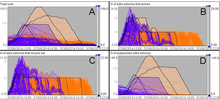
After this, the system runs the simulation. The results can be shown in several ways. The movements of individual vehicles can be played on an animated map, and the trajectories of the vehicles can be shown in a space-time cube. An animated map can also show the result as aggregated flows by time intervals. However, animated displays do not effectively support the assessment of the forecast. More useful are interactive time graphs linked to a map display through brushing. The time graphs show the evolution of several dynamic properties of the links: base load, extra load, total load, possible speed, number of vehicles that could move, number of suspended vehicles, etc. The simulation procedure also computes dynamic characteristics of the places, which can also be represented on time graphs. The use of the time graphs will be demonstrated by example in the next section.
4.2.4 Traffic Forecasting Example
announced that a severe storm is coming from the west and is expected to hit the coast around 18 o’clock. The weekend tourists are recommended to return to their homes. They should leave the coastal area before the storm comes. Many tourists decide to follow this recommendation. As a result, about 50,000 cars generate extra traffic in addition to the regular traffic on Saturday afternoon and evening.
In trying to simulate this scenario, we need to take into account the fact that our example data do not reflect the movements of all vehicles on the study territory but only the movements of 42,686 private cars; hence, the computed traffic intensities need to be scaled, as explained in section 2. From the data provider, we know that they track about 2% of the circulating private cars in Italy (the data are used for car insurance); however, the proportion of these cars in the whole traffic is unknown. A study has been conducted to find out whether these tracks can be used to infer the real traffic counts [54]. For a small set of road sections in Pisa, the researchers compared the counts of the tracked vehicles by time intervals with real traffic counts obtained from traffic sensors. The conclusion was that the sample of tracked vehicles is highly significant and can give a good approximation of the real traffic after appropriate scaling; however, the scaling functions differ for different road segments. Since real traffic counts for the entire underlying territory of our dataset are not available, valid scaling functions for all links cannot be derived for our specific case study. However, this does not diminish the general value of our approach. It is obviously applicable when data refer to the entire population of vehicles or when scaling functions can be derived using additional data. We believe that the spread of traffic sensors will increase over time, and obtaining complete traffic counts will be less and less problematic.
For the current case, we apply the following approach. We assume that the movements of the 2% of the private cars for which we have data are representative of the whole population of the private cars. We want to forecast movement of 50,000 private cars in total, and we know that about 2% of these cars are present in the available dataset and are accounted for in our models. Based on this reasoning, we shall simulate the movement of 2% of the 50,000 private cars, i.e., 1,000 cars, and treat it as representative for the whole set of 50,000 cars.
In steps 1 and 2 of the scenario definition procedure, we need to specify the trip origins and destinations of the 1,000 cars. We have no data about the homes and weekend accommodations of real tourists. Earlier it was found that the spatial distribution of the most probable home locations of car drivers that could be extracted from the GPS tracks of their cars is very highly linearly correlated with the distribution of the resident population [28]. The most probable home locations have been determined as the most frequent locations of trip ends in the evening and night hours. Hence, the distribution of the trip ends in the evening and night can serve as a proxy for the resident population distribution, i.e., the counts of the evening trip ends in the places can be taken as the place weights for generating the spatial distribution of the possible trip destinations of the weekend tourists. Moreover, for the places located at the coast, these weights can be used for generating the spatial distribution of the supposed trip origins, assuming the number of tourists in a place to be proportional to the number of the place residents. This is a reasonable assumption since tourists usually stay in populated places.
By interacting with the map display, we divide the set of places into coastal and inland. Then we let the system automatically distribute 1,000 cars over the coastal places proportionally to the place weights, for which we take the average numbers of trip ends after 18:00. Analogously, we distribute the destinations of the car trips over the inland places. The results are shown on a map in Fig. 11 by violet and orange circles with the sizes proportional to the number of trips originating from the places (violet) and the number of trips ending in the places (orange). In our scenario, we prohibit the origin places to be also used as destinations, but, in general, this is not required.
In step 3, the system automatically matches the origins with the destinations as described previously. In step 4, we find suitable parameter settings for the vehicle routing by generating test routes for various origin-destination pairs and parameter values. After this, the system generates possible routes and chooses a route for each car. In Fig. 11, the result of the route generation and assignment is shown on the map in an aggregated form: for each link, the number of cars that will pass through it (link load) is shown by proportional width of a curved line. A small map fragment in the lower right corner demonstrates this variant of link depiction in more detail.
[Fig. 11. The distribution of the trip origins and destinations and the expected link loads.]
In step 5, we specify the time interval in which the cars will start moving: from 13:00 to 16:00 on the 7th of June 2014 (Saturday). We set that the trip starts will be normally distributed within this interval and that the simulation results need to be aggregated by 10-minute intervals. Then we start the simulation, which runs for 19 seconds, and then assess the simulation results. We see that the total time that will pass from the first vehicle starting moving (13:03) till the last vehicle arriving at its destination (23:15) will be 10 hours 10 minutes.
(D). The dynamics of these characteristics in the places are represented by lines colored in violet for the places located at the coast and in orange for the remaining places. We see that the last extra vehicles will leave the coastal places by 19:30, i.e., in 1.5 hours after the supposed storm start.
[Fig. 12. Simulation results aggregated by the places and 10-minutes intervals: total load (A), number of extra vehicles that arrived (B), number of extra vehicles that moved out (C), number of suspended extra vehicles (D). The lines corresponding to the coastal places are shown in violet and the remaining lines in orange.]
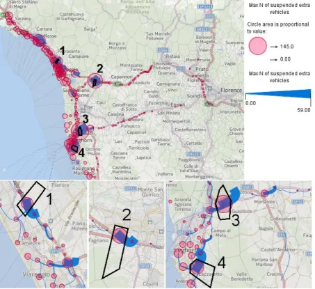
The time graph D shows us that in some places many cars will be suspended for long time. The lines corresponding to these places are highlighted in black. Two places are located at the coast and two are inland. The problematic places are highlighted in black and labeled by numbers on a map in Fig. 13, where the circles represent the maximal counts of suspended cars per time interval. The areas around the problematic places are shown in more detail at the bottom of Fig. 13. The maximal suspensions on the links are represented by the widths of the curved lines. The major suspensions will occur at motorway entrances near highly populated areas (1, 4) and on motorway junctions (2, 3).
[Fig. 13. The map shows the places (red circles) and links (blue curved lines) where the evacuating cars will be queuing.]
4.3 Develop Options
Since it will take too long for the evacuating cars to leave the coastal area, it is necessary to find possible interventions that can reduce the evacuation time. Two types of interventions are possible: (1) direct a part of the traffic to alternative roads that are expected to be less busy, and (2) on motorways, use one or more lanes going in the opposite direction as additional lanes for the evacuating cars. These actions can be introduced into a scenario in the following way. Traffic re-directing can be imitated by modifying link weights. Increasing the weights of links that are not heavily used will attract more traffic to these links. Decreasing the weights of overloaded links may divert a part of the traffic to other links, if reasonable alternative routes exist. Setting a link weight to zero imitates closing this link for traffic. Using additional lanes on motorways to speed up the movement of traffic in a particular direction is modeled by modifying the maximal numbers of vehicles that can pass through links (i.e., link capacities). For links going in the target direction, the capacities are increased, and for links going in the opposite direction, the capacities are decreased. The framework allows two ways of interactive modification of link properties: by selecting links on a map one by one and entering new values or by selecting a set of links and modifying their properties in a uniform way, e.g., by multiplying by a given factor.
After finishing a simulation run, the system allows the analyst to inspect the result as long as needed, then to modify the weights or capacities of some links, and then start a new simulation. The analyst does not need to perform again the full scenario definition procedure. The tool takes all settings from the previous run and only asks the user about the attributes specifying the altered link properties. Results of two simulation runs can be compared in two ways. First, the analyst can visualize the result of each run on an individual map and individual set of time graphs, put the maps and graphs side by side, and compare them visually using brushing and synchronous filtering to link the views. Second, the system can compute and visualize the differences between the results.
[Fig. 14. The impact of redirecting a part of the traffic to road SP24 passing Pisa is visualized as a change map.]
The circles represent the changes of the maximal counts of suspended cars in the places. The circle areas are proportional to the absolute differences. Positive changes (i.e., increases) are shown in semi-transparent red and negative changes (i.e., decreases) in cyan. The colors of the flow lines and circles have been chosen for making a good contrast on the map. We see that the maximal number of suspended cars in place 3 will decrease by 134 and, moreover, the maximal number of suspended cars in place 2 will also decrease by 19.
We visualize the new simulation results in time graphs, as in Fig. 12, and see that not only the number of suspended cars will decrease in places 2 and 3 but also the duration of the suspension. However, the total evacuation duration will increase by 1 hour and the time required for leaving the coastal area will increase by 10 minutes. Hence, the redirection of some traffic to SP24 solves the local problem in place 3 and alleviates the problem in place 2 but does not yield a global improvement of the evacuation time. Furthermore, the local improvement in place 3 will be annulled by increased suspensions in place labeled 5 located farther on the same road (Fig. 14).
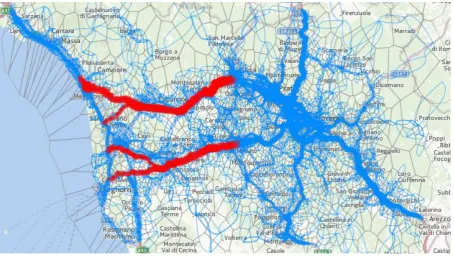
The next action we shall try is increasing the capacities of the inland-directed links located along the major roads through partial use of the opposite-going lanes of these roads for the evacuating cars. We expect that this can speed up the removal of the evacuating cars from the coastal places. We interactively select the links on the map display (the selected links are shown in red in Fig. 15) and multiply their capacities by factor 1.5. The capacities of the opposite links are multiplied by factor 0.5. This imitates using a half of the opposite link capacities for the movement out of the coastal area. After running the simulation with the modified link capacities, we observe large improvements in the evacuation from the coastal area. Time graphs, as in Fig. 12, show us that the evacuating cars will completely leave the coastal area by 19:00, which is 30 minutes earlier than in the original scenario. We select the coastal places where some cars will still be present after 18:00 and see that in most of them there will be no evacuating cars already by 18:20 and only in two places cars will be present till 18:50. By brushing the lines of these two places on the time graph and looking at a map, we find that they are located on a motorway junction near Viareggio. In Fig. 16, the numbers of cars that will leave the coastal places only after 18:00 are shown by proportional circle sizes. There will be 61 such cars (6.1% of the total number of simulated cars) in the two places near Viareggio and maximum 4 cars in all other places.
[Fig. 15. The links where the capacities will be increased by using opposite lanes are shown in red.]
[Fig. 16. The coastal places where some evacuating cars will still be present at 18:00 and later are marked by red circles with the sizes proportional to the numbers of these cars.]
Hence, re-routing the traffic and increasing the link capacities for the inland-directed movement will significantly speed up the evacuation from the risk area, but about 6% of the cars concentrating near Viareggio will not be able to leave the area before 18:00. We do not see any further opportunities for helping these cars to move out faster. It may be too dangerous for them to keep moving during the storm. A safer option may be to direct the cars suspended at the problematic junction to the nearest town Viareggio and provide the evacuees with shelters for staying until the storm ends.
We also investigate the movement of the evacuating cars beyond the coastal area. The time that will pass till the last car arrives at its destination will decrease by only 10 minutes. There will be three inland places where many cars will be suspended during long time intervals. One of them is place 2 near Lucca known from Figs. 13 and 14 and two other are located farther to the east. The places of suspensions are well visible in a space-time cube (Fig. 17) representing the simulated trajectories of the cars (the trajectories are colored according to their places of origin). The suspensions appear in the cube as vertical trajectory segments, which mean that the spatial positions do not change as the time passes. The three problematic places are marked in the cube by arrows and labeled 2, 6, and 7. Compared to the original scenario, the maximal number of suspended cars in place 2 will decrease from 115 to 80. In place 6, the maximal number of queuing cars will reach 55, and the congestion time will be quite long: from 14:30 till 21:10. Unfortunately, there are no further possibilities for improving the flow of the evacuating traffic through these places, as the opposite link capacities have been already used. Fortunately, the places are located out of the most dangerous area; hence, the congestions will not have dramatic consequences. Place 7 is located yet farther to the east. The congestion time in it (from 15:00 to 19:20) will be much shorter than in place 6.