Stabilised finite element methods for the Oseen problem on anisotropic quadrilateral meshes

the Oseen problem on anisotropic

quadrilateral meshes

∗

Gabriel R. Barrenechea

Department of Mathematics and Statistics,

University of Strathclyde,

26 Richmond Street, Glasgow G1 1XH, Scotland

and

Andreas Wachtel

Departamento acad´emico de Mat´ematicas,

ITAM – Instituto Tecnol´ogico Aut´onomo de M´exico

June 20, 2017

In this work we present and analyse new inf-sup stable, and stabilised, finite element methods for the Oseen equation in anisotropic quadrilateral meshes. The meshes are formed of closed parallelograms, and the analysis is restricted to two space dimensions. Starting with the lowest order Q21 ×P0 pair, we first identify the pressure components that make this finite element pair to be non-inf-sup stable, especially with respect to the aspect ratio. We then propose a way to penalise them, both strongly, by directly removing them from the space, and weakly, by adding a stabilisation term based on jumps of the pressure across selected edges. Concerning the velocity stabilisation, we propose an enhanced grad-div term. Stability and optimal a priori error estimates are given, and the results are confirmed numerically.

Keywords: Oseen equation, stabilised finite element method, anisotropic quadrilateral mesh

1 Introduction

In this paper we discuss stabilised finite element methods for the Oseen problem on highly anisotropic meshes. This equation appears, for example, in the iterative solution

∗

This research was supported by the Leverhulme Trust under grant RPG-2012-483.

†

[email protected]

‡

[email protected]

1

of the Navier–Stokes equations. As it is the case with the Navier-Stokes equation, when solving the Oseen problem numerically three different aspects can affect the quality of the numerical solution, and then need to be treated. One is a compatibility condition between velocity and pressure spaces, namely the inf-sup condition, that requires to be satisfied, or circumvented. In addition, if the mesh is not refined enough, then the local P´eclet number is much larger than one (i.e., if the problem is convection-dominated), then the numerical solution usually presents spurious, non physical, oscillations. Finally, even if the solution to the continuous equation is divergence-free, usually the discrete solution is not. This can affect (sometimes dramatically) the quality of the numerical solution, especially when the Navier-Stokes equations are coupled to, say, temperature equations.

We start by discussing the first restriction mentioned in the previous paragraph. The first approach was to design pairs of velocity and pressure spaces that satisfy the inf-sup condition. For extensive reviews of such an approach on shape-regular meshes we refer to [GR86, BBF13], and the references therein. Now, the simplest finite element pairs, namely, equal-order interpolation for velocity and pressure, or the Q21 ×P0 element, are not inf-sup stable. Then, in the mid eighties the idea of stabilisation appeared in order to circumvent this restriction. Examples of stabilised methods are PSPG methods, introduced for shape-regular meshes in [HFB86], and extended to anisotropic meshes in [MPP03, Bla08]. Later on, different approaches have been proposed to stabilise this restriction, including Residual-Free Bubbles, or enriched finite element methods (see, e.g., [BBF93, ABV06]), and Local Projection Stabilised (LPS) methods (see [BB01]). Alternatively, and as an attempt to analyse some of these methods in a unified manner, the idea of minimal stabilisation was proposed in [BF01]. This approach consists of splitting the pressure space into the sum of a stable part and an unstable part. Then, a stabilising term is added to the formulation to control the unstable part of the pressure space, hence restoring stability. This approach provided a different interpretation of some older methods, e.g., [PS85], the local jumps stabilisation [KS92], and pressure projection [BDG06] (see [Bur08] for a unified presentation of this idea). In addition, this approach was recently used to design new inf-sup stable, and stabilised, finite element methods for the Stokes problem on anisotropic meshes in [ABW15] (modifying a decomposition given previously in [AC00]). This last work concerned for the pairsQ2_k+1×P2_k−1, k≥1,

and then does not cover the lowest order case. For the latter case, and in the context of the Stokes problem, the local jump method from [KS92] was recently extended to anisotropic meshes without corner patches in [LS13], and to meshes containing corner patches in [BW15].

where the method is applied to the Oseen and Navier-Stokes equations using equal order

Q21×Q1 elements on anisotropic, structured, quadrilateral meshes.

Concerning the satisfaction of the divergence-free character of the velocity field at the discrete level, the numerical velocities obtained using inf-sup stable elements are discretely divergence-free by definition, although this might not be enough in some ap-plications. Stabilised finite element methods, on the other hand, do not satisfy this property, even when discontinuous pressures are used, due to the pressure jumps added to the formulation. One possibility is to propose a post-processing of the discrete ve-locity, by means of the lowest order Raviart-Thomas element, as it has been done, for instance, in [BV10] in shape-regular triangular meshes. Another possibility to address this issue is to add a grad-div stabilisation term, this is, a consistent term of the form γ(divu,divv)Ω, whereγ >0 is a stabilisation parameter. The introduction of this term was first proposed in [FH88] and it has been extensively used to improve the control of the discrete divergence for the Navier-Stokes equation and coupled problems (see, e.g., [LM+09, GL+12]). An analysis of this method can be found in [OR04], and, espe-cially in [JJ+14], where a very detailed analysis and discussion on the selection of the stabilisation parameter is presented.

The objective of this paper is to propose and analyse a stabilised finite element method for the Oseen problem on anisotropic quadrilateral meshes containing corner patches. The stabilisation terms related to the pressure are those from the method given in [LS13], supplied with appropriate (selected) edge terms to make the method stable in-dependently of the aspect ratio, and the presence of corner patches. Since the method from [LS13] is based on the refinement of a macro-element mesh, then the present ap-proach also requires some level of structure of the meshes. Concerning the stabilisation mechanisms for the convection, the stabilising terms are based on the LPS stabilisation ones, augmented with a grad-div/LPS term (this is, a term penalising the fluctuations of the divergence, rather than the divergence itself, as it was done, e.g., in [BV10]). One extra feature of the method is that the velocity is locally mass-conservative, at least in the macro-elements, and this fact is further imposed by the grad-div stabilisation term. The analysis of the method follows the very general approach given in [MT15], supplied with the new proof of stability for the pressure, which generalises the one presented in [BW15].

2 Notation and preliminary results

Throughout, constants with capitalC are independent of data, whereas constants with a lower casec may depend on data. Both the instances of C and c are independent of all geometric properties of the mesh. We use standard notation for Sobolev spaces; for instance, for ω _⊂ R2, | · |1,ω and k · k0,ω denote the H1(ω)-seminorm and L2(ω)-norm, respectively, and L2₀(ω) denotes the space of functions in L2(ω) with zero mean in ω. Furthermore, by (v, w)_ω we denote the inner product inL2(ω). Vector-valued spaces are bold-faced, e.g.H1₀(ω) = [H1

0(ω)]2, but the same notation for norms and inner products is used.

2.1 The problem of interest

Let Ω_⊂R2 be a polygonal, bounded and connected domain. Then, givenf ∈L2(Ω) we

consider the following Oseen problem

−ν∆u+ (b_{· ∇})u+σu+_∇p=f in Ω,

divu= 0 in Ω,

u= 0 on∂Ω,

(2.1)

subject to_hp_iΩ = 0, where _hq_iω denotes the meanvalue of q overω _⊂Ω. For simplicity we suppose ν is a positive viscosity constant, σ is a non-negative constant and b ∈

H(div,Ω)_∩L∞(Ω), with divb= 0, is a given velocity field. The weak formulation of Problem (2.1) is given by:

Find (u, p)∈V×Q:=H1₀(Ω)×L2₀(Ω) such that

B((u, p),(v, q)) = (f,v)_Ω for all (v, q)∈V×Q , (2.2) where

B((u, p),(v, q)) :=a(u,v)₋(divv, p)_Ω−(divu, q)_{Ω ,} (2.3) a(u,v) :=ν(_∇u,_∇v)_Ω+ ((b_{· ∇})u,v)_Ω+σ(u,v)_{Ω .} (2.4) Using integration by parts and divb= 0 the bilinear form ainduces the norm

kv_k2_a:=a(v,v) =ν_|v_|12_,Ω+σ_kv_k02_,Ω for all v _∈V . (2.5) Ifσ = 0, then thanks to thePoincar´e inequality

∃CΩ >0 , ∀v ∈V : kvk_0,Ω ≤CΩ|v|_{1,Ω ,} (2.6)

k·ka remains a norm. The following continuity estimates will be of use in the stability and convergence analysis.

Lemma 2.1. For all w,v _∈V the following inequalities hold

kv_k2_0,Ω≤ C

2 Ω ν+σC2

Ω

kv_k2_{a ,} (2.7)

and

a(w,v)_≤cakwka|v|1,Ω where ca:=

ν+σC_Ω2 +b_∞,ΩCΩ

ν+σC2 Ω

1/2 (2.8)

Proof. Using the Poincar´e inequality (2.6) we get

kvk2a≥

ν C2

Ω

kvk20,Ω+σkvk

2 0,Ω =

ν+σC2 Ω C2

Ω

kvk20,Ω ,

which proves (2.7). To prove (2.8), we consider (2.4), (2.5) and estimate term by term. First, we obtain

ν(_∇w,_∇v)_Ω+σ(w,v)_{Ω ≤}ν_|v_|2_1,Ω+σ_kv_k02_,Ω1/2_kw_ka

≤ ν+σC_Ω21/2

|v_|1,Ωkw_ka.

Now, integrating by parts, using divb= 0, and (2.7) we get

|((b_{· ∇})w,v)_Ω|=_|((b_{· ∇})v,w)_{Ω| ≤}b_∞,Ω|v|1,Ωkwk0,Ω≤

b_∞,ΩCΩ

ν+σC_Ω21/2|v|1,Ωkwka.

(2.9)

Adding these last two estimates proves (2.8).

Finally, the inf-sup (or LBB) condition

inf q∈Q_vsup_∈V

(q,divv)_Ω

|v_|1,Ωkq_k0,Ω ≥βΩ >0, (2.10)

holds, see for instance [GR86, pp. 58–61]. With these last ingredients, and applying standard arguments in variational problems with constraints (see, e.g., [GR86]), we conclude that the Oseen problem (2.2) has a unique solution.

2.2 Partitions and finite elements

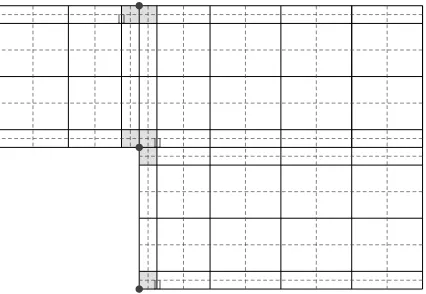
In order to construct partitionPwe start from an initialmacro element partitionMthat consists of closed parallelograms and satisfies a maximal angle condition. We suppose thatMis conforming, that is, the non-empty intersection ofM, M0 ∈Mis either a single common point or a shared edge. It is worth mentioning that partition M is allowed to be highly anisotropic and containcorner patches, that is, a drastic change of stretching in two directions may occur in some parts of the mesh. See for example the areas around the shaded cells in Figures 1–3.

We define the partitionPas a uniform refinement ofM, and state the main definitions and properties ofP:

• Let _EP denote the set of interior edges of P. Throughout we use M to denote an element ofMand refer to it asmacro element, and useK to denote elements ofP. Additionally, we use_|ω_|to denote the area ofω_⊂R2 and |e|to denote the length

of an edge.

• The uniform refinement splits each macro elementM _∈MintoK1, K2, K3, K4∈P, such that_|Ki|=|M|/4 (i= 1, ..,4), see Figure 1.

• The aspect ratio of a cellK ∈Pis defined by%K := mine⊂∂K|K|/|e|2. The mesh aspect ratio is defined by%:= minK∈P%K.

• Let C be the set of corners, that is, nodes c of the mesh M towards which the mesh is refined, denoted by filled circles in Fig. 1–3. For c _∈ C, we denote by ωc the area around c that is partitioned in a shape-regular way (shaded in Fig. 1–3). Moreover, for every c ∈C, we select a single edge γc ∈ EP that separates a small corner macro element (shaded) from a highly stretched neighbouring macro element, e.g., the embraced edges in Fig. 1–3. The selected edgesγc are collected in the set EC.

Even if the above-stated hypotheses allow more general situations, from now on we will restrict our analysis to meshes of the type depicted in Figures 1–3. In particular, we will not consider the case of graded meshes or meshes in which the change between ωc and the complement is more subtle than the one from these figures.

h h

H H

h h

H H

J K

Fig. 1 PartitionM(left) andP(right). We call thisMcorner patch.

λ

J K

λ

J K

λ

J K

Fig. 2 Corner patches on [0, λ+H]2 whose corners were refinedrtimes (r= 0,1,2).

It is worth mentioning that the condition “P arises from a uniform refinement of M” still allows local (macro-element based) refinements, as described in [LS13]. In particular, instead ofM, an initial partitionMr, that contains corner patches that have been refined uniformly r-times, may be used as a macro-element mesh for P, cf. Figure 2, where the partitions M0,M1,M2 and P0,P1,P2 have been depicted. To lighten the notation, we remove the subindexr whenever it is clear from the context, but we keep in mind that the partitions Mand Phave been refined, as in Fig. 2, r times.

Finally, we define the finite element spaces

V`,P:=

J K J K

J K

Fig. 3 An anisotropic mesh for flow over step.

and

Q_P:={q_∈Q: q_{|K ∈}P0(K) for all K∈P}, (2.12)

where, as usual, Q`(K) denotes the space of polynomials of degree less that, or equal to, ` in each variable, and P0(K) denotes the space of constant functions in K. We seek an approximation of the solution (u, p) of Problem (2.1) within the discrete space

V1,P×QP.

2.3 Preliminary results

It is a well known fact thatV1,P×QPis not inf-sup stable, even on shape-regular meshes.

On the other hand, sinceV1,P andV2,M share the same degrees of freedom,V1,P×QM is inf-sup stable. Now, sinceMcontains corner patches, then the inf-sup constant of the latter pair is affected by the aspect ratio ofM. More precisely, applying the results from [AC00] (see also [ABW15]) we conclude that

inf q∈QM

sup v∈V1,P

(q,divv)_Ω

|v_|1,Ωkq_k0,Ω =βM≥C

√

% , (2.13)

and this bound is sharp. This issue is then solved in the next result where we impose a minimal set of additional constraints to obtain a uniformly inf-sup stable subspaceG of Q_M. In this lemma, and thereafter, for a functionq,_Jq_Kγ will denote its jump across the edgeγ.

Lemma 2.2. Let G_⊂Q_M⊂Q_P be the space defined by

G:=nq∈Q_M: _Jq_Kγc = 0 for every γc∈ E_C

o

. (2.14)

Then, the following inf-sup condition holds

sup v∈V1,P

(divv, q)_Ω

|v_|1,Ω ≥βGkqk0,Ω for all q ∈G , (2.15)

see Figure 2). Equivalently, the following inf-sup deficiency holds

sup v∈V1,P

(divv, q)_Ω

|v_|1,Ω ≥βGkΠGqk0,Ω− kq−ΠGqk0,Ω for all q ∈QP, (2.16)

where ΠG:QP→G stands for the L2(Ω)-projection onto G.

Proof. The proof follows a similar path as in [ABW15] allowing the extension to re-fined corner patches. For completeness we include an abridged version here. We first prove (2.15). Since G_⊂Q_M, we have βG ≥βM. For the alternative βG ≥C/2r, let us define

Q∗_M:=

q _∈Q_M: _hq_iω

c = 0 for c∈C .

Let now q∗ _∈ Q∗_M. As in [ABW15, Corollary 3.1] there exists v∗ _∈ V1,P such that

v∗|ωc ∈H

1

0(ωc) for everyc∈C, and

(divv∗, q∗)_Ω =_kq∗_k2_0,Ω and _|v∗_{|1,Ω ≤}Cˆ_kq∗_{k0,Ω ,} (2.17)

where ˆC >0 depends only on Ω. In particular, this constant ˆCis independent ofr. Next, we decomposeq∈Gintoq = Π_Cq+q∗ where Π_Cq|ωc (forc∈C) and ΠCq|Ω\(∪c∈Cωc) are

constants, and q∗ _∈ Q∗_M. Then, since (divv∗,Π_Cq)_Ω = 0 we get (divv∗, q) = _kq∗_k2_0,Ω. Therefore, (2.17) implies (2.15), once the following is proved

kq_k0,Ω≤C2r_kq∗_{k0,Ω .} (2.18)

As in [ABW15, Lemma 3.2] we conclude that kΠ_Cqk20,Ω ≤C

P

c∈C|ωc| hJq∗Ki2_γc. Noting that γc ⊂Mc∩Mc0, with Mc, Mc0 ∈M,|Mc| ≤ |Mc0|, and using that|ωc| |Mc|−1 = 22r, each of these jumps is bounded as

|ωc| hJq∗Ki2_γc≤C|ωc| |Mc|−1kq∗k2_0,Mc∪M0

c ≤ C2

2r_kq∗_k2 0,Ω ,

and then (2.18) follows.

Finally, given (2.15), the proof of [ABW15, Lemma 4.1] implies (2.16). The reverse follows using only ΠGq =q forq ∈G. This finishes the proof.

Remark 2.3. We stress the fact that βG only depends on how refined the partition M

is. This is reflected by the factor 2r _{in β}

G. This unfortunate behaviour can be solved

easily by limiting the number of refinements and instead movingλcloser to the nodes c, since βG is bounded below by a constant independent of λ.

Lemma 2.4. Let G ⊂ Q_P be defined as in Lemma 2.2. Then, there exists uI ∈ V1,P

such that

(div(u₋uI), q)_Ω = 0 for all q∈G , (2.19)

and

|u₋uI|1,Ω ≤2(1 +βG−1)_v inf

P∈V1,P|

u₋v_{P|1,Ω .} (2.20)

Proof. Let (φ_P, χ_P)∈V1,P×Gbe the solution of the following auxiliary problem: (∇φ_P,∇v)_Ω−(divv, χ_P)_Ω = (∇u,∇v)_Ω for all v∈V1,P,

(divφ_P, q)_Ω = (divu, q)_Ω for all q_∈G . (2.21) The well-posedness of this problem is a consequence of (2.15). Then, defininguI:=φ_P, (2.19) follows immediately from (2.21). Moreover, since (uI, χP) is a finite element

approximation of (u,0), (2.20) follows by standard arguments, see e.g. [GR86, p.115], or [Joh17, Lemma 3.60 and Theorem 4.21].

Remark 2.5. We finish this section by providing some more insight in the behavior of the inf-sup constant β_M as the corner patches get refined. Our aim is to show that this constant, not only doesn’t degenerate, but it actually increases with r. We remind that we have dropped the subscript r whenever it is clear from the context, but we keep in mind that the macro-element patch M has been refined r times.

First, from (2.13) and (2.17) we conclude that the spurious mode on the (refined) corner patch in Figure 2 is given by the function connecting the (uniformly stable) average free spaces on ωc:= [0, λ]×[0, λ]and Ω\ωc, i.e.

qB :=χωc−

|ωc|

|Ω\ωc|

χΩ\ωc.

Let us first define the quantity

˜

βr:=kqBk−_0,1_Ω sup v∈V1,P

(qB,divv)Ω

|v_|1,Ω .

Next, using (2.17) and the definition of the space Q∗_M we can easily see that

sup v∈V1,P

(divv, q)_Ω

|v_|1,Ω ≥

1 ˆ C

q−(q, qB)Ω

kqBk20,Ω

qB

0,Ω

, (2.22)

for allq _∈Q_P. Then, using [Joh17, Theorem 3.89], we conclude that

β_M= Cˆ−

1

1 + ˆC−1_{+ ˜β} r

˜

βr. (2.23)

Thus,β_Mis an increasing function ofβ˜r. Moreover, since the spaceV1,P becomes richer asr increases, thenβ˜rincreases withr. Thus, we haveβM0 ≤βM1 ≤. . .≤βMr ≤C

√_ρ

0,

where ρ0 is the aspect ratio of the initial macro-element partition M0. In Table 1 below

2.4 Numerical confirmation (part 1)

In this section we show the improvement of βG over βM. For simplicity we restrict

the presentation of βG to partitions on the unit square Ω = (0,1)×(0,1). To this end, we define a parametrized (by λ > 0), refined corner patch Mr as the tensor-product of the following one-dimensional interval subdivision of [0,1]. The parameter λ < 1/2 separates a coarse and a fine region in [0,1]. The interval [0, λ] is split into 2r intervals of length λ/2r _{and [λ,1] remains unsplit. Figure 2 shows these macro-element meshes}

Mr forr = 0,1,2 as continuous lines. The subspace G⊂QM additionally imposes the

continuity across the edges in EC for each case.

We have computed βG and βM for different levels of refinements while lettingλ→0.

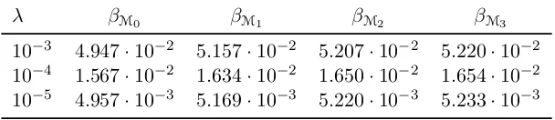
The results are depicted in Figure 4. The constants βG remain bounded below by a constant independent ofλ, as predicted by Lemma 2.2. Moreover, to confirm the claim made in Remark 2.5 we have computed the constant β_M for different values of r and different values ofλ. We report the obtained values in Table 1 where it can be seen that the value of the inf-sup constantβ_M grows withr.

10−6 ₁₀−5 ₁₀−4 ₁₀−3 ₁₀−2 ₁₀−1

λ (r= 0) 10−2

10−1 100

βM0 βG0

10−6 ₁₀−5 ₁₀−4 ₁₀−3 ₁₀−2 ₁₀−1

λ (r= 1) 10−2

10−1 100

βM1 βG1

10−6 ₁₀−5 ₁₀−4 ₁₀−3 ₁₀−2 ₁₀−1

λ (r= 2) 10−2

10−1 100

βM2 βG2

Fig. 4 Constants βG andβM, forr= 0,1,2.

Table 1. A numerical confirmation of Remark 2.5

λ β_M0 β_M1 β_M2 β_M3

10−3 _4.947·10−2 _5.157·10−2 _5.207·10−2 _5.220·10−2 10−4 1.567·10−2 1.634·10−2 1.650·10−2 1.654·10−2 10−5 4.957_·10−3 5.169_·10−3 5.220_·10−3 5.233_·10−3

3 The stabilised method for the Oseen equation

The stabilised method proposed in this work reads: Find (u_P, p_P)∈V1,P×QP such that

B_s((u_P, p_P),(v_P, q_P)) = (f,v_P)_Ω for all (v_P, q_P)_∈V1,P×QP, (3.1)

where

Bs((u, p),(v, q)) :=B((u, p),(v, q)) +sv(u,v)−sp(p, q), (3.2) and sv and sp are symmetric, positive semi-definite bilinear forms aimed at stabilising velocity and pressure, respectively. In order to prove stability and a priori estimates we need to make assumptions on sv and sp. For this purpose, we define

|v_|2_s

v :=sv(v,v) and kvk 2

a+s:=kvk 2 a+|v|

2

and the bilinear form

sdiv_v (u,v) := X K∈P

γK(κK(divu), κK(divv))_K , γK ≥0, (3.4)

whereκω := id− h·iω denotes the fluctuation operator. We now state the main assump-tions on sv and sp.

Assumption 3.1. Letv,w_∈V. There exists a positive constantcs, which may depend

on the data, but is independent of the mesh, such that

sv(w,v)≤cs|w|_sv|v|_{1,Ω .} (3.5)

Furthermore,sv is assumed to satisfy

sdiv_v (v,v)≤sv(v,v), (3.6)

where sdiv_v is given by the LPS-like term (3.4).

We remark that, thanks to the above hypotheses then sv(·,·) satisfies the following Cauchy-Schwarz inequality

sv(w,v)≤sv(w,w)1/2sv(v,v)1/2. (3.7) With the above constants we define

α:= 1

c2 a+c2s

, (3.8)

withca and cs from (2.8) and (3.5), respectively. Then, the pressure stabilisation term is given by

sp(p, q) := αp

4

X

M∈M

SM(p, q) + αp

4

X

γc∈EC

Sγc(p, q), (3.9a)

withαp≥α, and

SM(p, q) :=

X

e∈EM

|M|

4|e|(JpK,JqK)e , (3.9b)

Sγc(p, q) :=

min{|K|,|K0|}

|γc|

(_Jp_K,_Jq_K)_γc , (3.9c)

whereK, K0∈Pare such that γc=K∩K0.

Remark 3.2. For q _∈ G we realise that sp(q, q) = 0. Consequently, sp only acts in

4 Stability of the method

This section is devoted to proving that Method (3.1) is stable with a stability constant depending only onβG. The norm that will be used is given by

|||(v, q)_|||2:=kv_k2_a+s+α_kq_k2_0,Ω+sp(q, q). (4.1) The next result is the first step towards stability.

Lemma 4.1. Letq_P∈Q_P,p∈H1(Ω)andΠGbe the projection from Lemma 2.2. Then,

the following holds

1

34αpkqP−ΠGqPk 2

0,Ω ≤sp(qP, qP), (4.2)

sp(qP, qP)≤Cαp

X

K∈P

kp−q_Pk20,K+|e1,K|2k∂t1pk

2

0,K +|e2,K|2k∂t2pk 2 0,K

, (4.3)

where e1,K and e2,K are two non-parallel edges ofK, ∂ti(i= 1,2)are partial derivatives

in their directions, and C is a constant independent of mesh, angles, and data.

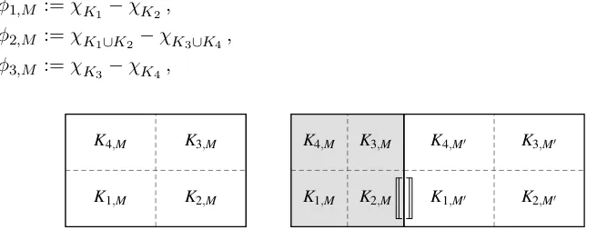
Proof. We start with (4.2). This proof uses notation and conventions from Figure 5. Our assumptions on the partitions P and M imply that every selected edge γc ∈ EC (the embraced edge in Figure 5-right) satisfies γc⊂M∩M0 where M, M0 ∈ M and

|M_{| ≤ |}M0_|. For readability we defineωγc := M∪M0. Now, from its definition ΠGq is

given by

ΠGq

M =

(

hqiωγc ifM ⊂ωγc,

hqiM otherwise.

(4.4)

Therefore, bound (4.2) follows once we prove the local bounds

2αpkqP− hqPiMk20,M ≤αpSM(qP, qP), (4.5a) 2

17αp

qP− hqPi_ω

γc

2

ωγc ≤αp SM +SM

0+S_γ

c

(q_P, q_P). (4.5b)

The first estimate has been proven as part of [LS13, Lemma 3.2]. We include here a different proof which supplies us with notation and arguments for (4.5b). Let M _∈ M be a macro element such thatM 6⊂ωγc,γc∈ EC. Since all cells K ⊂M have the same

area, an orthogonal basis ofQ_P∩L2₀(M) is given by (cf. Figure 5, left)

φ1,M :=χK1−χK2,

φ2,M :=χK1∪K2 −χK3∪K4, φ3,M :=χK3−χK4,

(4.6)

K1,M K2,M K3,M K4,M

K1,M K2,M K3,M K4,M

s {

K1,M′ K₂,M′

K3,M′

K4,M′

whereχ_ω is the characteristic function of ω. Below, we omit the subscriptM when it is clear from the context.

Let ra:= (qP− hqPiM)|M ∈QP∩L20(M). Then,ra=P3_i=1αiφi with appropriate co-efficients αi, and using|Ki|=|M|/4,(i= 1, . . . ,4), the definition ofSM,JraK_e ∈P0(e),

and orthogonality of the basis we get

SM(qP, qP) =SM(ra, ra) = | M_|

4

X

e∈EM 1

|e|kJraKk

2 0,e =

|M_|

4

X

e∈EM

JraK2_e

= |M| 4

(2α1)2+ (2α2−α1−α3)2+ (2α3)2+ (−2α2−α3−α1)2

= |M| 4

4α2₁+ 4α2₃+ 8α2₂+ 2(α1+α3)2

= 2_kα1φ1k2_0,M+ 2kα3φ3k2_0,M+ 2kα2φ2k2_0,M +| M_|

2 (α1+α3) 2

= 2_krak20,M +

|M|

2 (α1+α3)

2_{, (4.7)}

which proves (4.5a).

To prove (4.5b), we fix an edge γc∈ EC and let rb := qP− hqPiωγc

ωγc. Then

rb =α0φ0+ra+r0a,

where φ0 =|M|−1χM − |M0|− 1

χ_M0, r_a =

P3

i=1αiφi,M and r0a =

P3

i=1α0iφi,M0. Using

(4.7), the definition ofφ0 and |K| ≤ |K0|(since|M| ≤ |M0|) we get

SM +SM0 +S_γ

c

(q_P, q_P)≥2krak2_0,M + 2

r_a0

2 0,M0 +

|K_|

|γc|kJ

rbKk20,γc . (4.8)

It only remains to bound the last term. Using _JrbKγc,Jφ0Kγc ∈P0(γc) and the linearity

of the jump, followed by 2ab≤ 1

2a2+ 2b2 we obtain

kJrbKk20,γc

|γc|

=_Jα0φ0Kγc+α2−α

0

2−α1−α01

2

=_Jα0φ0K2_γc+ 2Jα0φ0K_γc α2−α02−α1−α01

+ α2−α02−α1−α01

2

≥ 1₂Jα0φ0K2γc− α2−α

0

2−α1−α01

2

≥ 1₂Jα0φ0K2γc−4 α

2

2+α022+α21+α012

,

and conclude withε <1 and_|K_|=_|M_|/4

|K|

|γc|kJ

rbKk20,γc ≥ε

|K|

|γc|kJ

rbKk20,γc ≥

ε

8|M|Jα0φ0K 2

γc−ε|M| α

2

2+α022+α21+α012

. (4.9)

Now, using the definition ofφ0 and |M| ≤ |M0|we get

|M_|Jα0φ0K2γc =α

2 0|M|

1

|M|+

1

|M0_|

2

≥α2₀

1

|M|+

1

|M0_|

and

|M_| α2₁+α₁02+α2₂+α0₂2

≤ |M_|(α2₁+α2₂) +

M0

(α0₁2+α0₂2)

≤2 krak20,M +

r_a0

2 0,M0

.

(4.11)

Choosing ε := 16₁₇, inserting (4.9)–(4.11) into (4.8) and using that φ0 is orthogonal to φi,M,φi,M0, i= 1,2,3 leads to

SM+SM0+S_γ

c

(q_P, q_P)_≥ 2 17 krak

2 0,M+

r0_a

2

0,M0+kα0φ0k

2 0,ωγc

= 2 17krbk

2

0,ωγc , (4.12)

which proves (4.5b).

Finally, using p_∈H1(Ω), _Jp_Ke = 0 a.e. on e_{∈ EP}, the trace estimate (9.1) (see the appendix for a proof), and the fact that q_P is a piecewise constant function, we bound each jump as follows:

|K_|

|ej|kJ

p₋q_PKk2_0,e j ≤2

X

K:ej⊂K

kp₋q_Pk0,Kkp₋q_Pk0,K + 2_|ei| kti· ∇pk0,K

≤4 X

K:ej⊂K

kp−q_Pk20,K+|ei|2kti· ∇pk20,K

,

whereei ⊂K is an incident edge to ej (i.e. i= 1, j = 2 ori= 2, j= 1). Then, we sum over the edges across whichsp contains jumps and note for eachK∈P, thatsp contains jumps across at least two and at most three different edges which proves (4.3).

We now present the main stability result.

Theorem 4.2. Let sv satisfy (3.5), let |||·||| be defined by (4.1), and sp by (3.9) with αp ≥α. Then,

sup (v,q)∈V1,P×QP

Bs((w, r),(v, q))

|||(v, q)||| ≥µs|||(w, r)||| for all (w, r)∈V1,P×QP, (4.13)

where µs = β_G2/[2(1 +βG)(35 + 34βG)] where βG is the constant from (2.15). Hence,

Problem (3.1) is well-posed.

Proof. Let (w, r)_∈V_1,P×Q_P be given. First, from the definition ofB_s it follows that

Bs((w, r),(w,−r)) =kwk2_a+s+sp(r, r). (4.14) Additionally, givenwδ ∈V1,P, using (2.8), (3.5) and α:= 1/(c2a+c2s) we get

B_s((w, r),(−wδ,0)) = (a+sv)(w,−wδ) + (divwδ, r)Ω

≥ −pc2

a+c2skwka+s|wδ|1,Ω+ (divwδ, r)Ω

≥ −1

2kwk 2 a+s−

1 2α|wδ|

2

1,Ω+ (divwδ, r)Ω. (4.15) Next, we choosewδ. By (2.16) there existsz ∈V1,P such that |z|1,Ω= 1 and

Definingwδ:=δαkrk0,Ωz withδ >0 to be chosen, this last estimate, (4.2) andα≤αp give

(divwδ, r)Ω≥βGδαkrk20,Ω−(1 +βG)δαkrk0,Ωα−p1/2C1−1/2sp(r, r)1/2

≥βGδαkrk20,Ω−

α 2C1

δ2(1 +βG)2krk20,Ω− 1

2sp(r, r), (4.16) and _|wδ|1,Ω = δαkrk0,Ω whereC1 = 1/34. We then define (v, q) := (w−wδ,−r), and (4.14), (4.15) and (4.16) yield

B_s((w, r),(v, q))≥ 1

2

h

kwk2a+s+sp(r, r)

i

+

βG−

δ(1 +βG)2 2C1

δαkrk20,Ω− 1 2α|wδ|

2 1,Ω

= 1 2

h

kw_k2_a+s+sp(r, r)

i

+βG

1₋δ(1 +βG) 2

2C1βG − δ 2βG

δα_kr_k2_0,Ω

≥ δβ₂G kw_k2_a+s+sp(r, r) +αkrk20,Ω

,

where the choiceδ :=βGC1/(C1+ (1 +βG)2) =βG/(1 + 34(1 +βG)2) andδβG≤1 imply the last estimate. On the other hand, using (2.8) and (3.5) showskzka+s≤α−1/2|z|1,Ω for all z_∈V1,P. Therefore, the definition ofwδ and |||·|||give

|||(v, q)_{||| ≤ |||}(w, r)_|||+_kwδk_a+s≤ |||(w, r)|||+δα1/2krk_0,Ω≤(1 +δ)|||(w, r)|||,

which proves the stated stability condition and the result withµs=δβG/(2 + 2δ).

Remark 4.3. It is important to remark that the stability constant µs only depends on βG, which is bounded below by a constant independent of the mesh aspect ratio. Therefore, µs is independent of the physical coefficients of the problem, and the aspect ratio of the

triangulation. Furthermore, the stability estimate (4.13) is valid independently of the relation of ca and cs. In [MT15] velocity stabilisation terms that satisfy (3.5) with cs ≤ Cca are used. We have chosen to avoid that assumption, since, as it has been

shown in [JJ+14], a large stabilisation parameter in the grad-div term may be beneficial in some cases.

5 A-priori estimates

This section is devoted to the a-priori analysis of (3.1). We use ΠQP:L

2_{(Ω) → Q}

P to

denote the L2-projection intoQ_P satisfying

(p₋ΠQPp,1)_K = 0 for all K∈P. (5.1)

Theorem 5.1. Let us suppose the solution (u, p) of (2.2) satisfies p _∈H1_{(Ω). Let s} v

satisfy Assumption 3.1 and let sp be defined by (3.9) with αp ≥α. Then, if uI ∈V1,P

is the interpolant defined in Lemma 2.4, then

|||(u₋u_P, p₋p_P)_{||| ≤}C(1 +µ−_s1)

sv(u,u) +sv(u−uI,u−uI) +σku−uIk20,Ω

+X

K∈P

1

α+αp

+ν+ b 2

∞,KCΩ2

ν+σC2 Ω

|u−uI|21,K

+α+αp+ 1 ν+γK

kp₋ΠQPpk

2

0,K +αp

X

i=1,2

|ei,K|2k∂tipk

2 0,K

1/2

where ei,K, ∂ti(i= 1,2)are defined as in Lemma 4.1, and the constantC is independent

of mesh and data.

Proof. As usual, we split the error as follows

(u₋u_P, p₋p_P) = (u₋uI, p−ΠQPp)−(uP−uI, pP−ΠQPp) =: (ηv, ηp)−(ξv, ξp). Using (3.3) the interpolation error satisfies

|||(η_v, ηp)|||2 =ν|ηv|21,Ω+σkηvk20,Ω+sv(ηv,ηv) +αkηpk2_0,Ω+sp(ηp, ηp).

The only term in the above expression that is not included in (5.2) is the last one. But, similar to (4.3), this term can be bounded by the last two in (5.2).

To bound the discrete error (ξ_v, ξp), using Theorem 4.2 there exists (wP, rP)∈V1,P×QP with_|||(w_P, r_P)_|||= 1 satisfying

µs|||(ξv, ξp)||| ≤Bs((ξv, ξp),(wP, rP))

=B((η_v, ηp),(wP, rP))−sv(uI,wP) +sp(ΠQPp, rP),

(5.3)

where we used (2.2) and (3.1). We estimate the right-hand side term by term. Using (3.7), a Cauchy-Schwarz estimate for sp(·,·), and|||(wP, rP)|||= 1 shows

−sv(uI,wP) =sv(ηv,wP)−sv(u,wP)≤sv(ηv,ηv)1/2+sv(u,u)1/2,

sp(ΠQPp, rP)≤sp(ΠQPp,ΠQPp)

1/2_, (5.4)

and applying p _∈H1(Ω) and (4.3) the right-hand sides of the last two inequalities are bounded by the first two and last two terms of (5.2). Next, using the Cauchy-Schwarz inequality and (2.7) we get

ν(∇η_v,∇w_P)_Ω+σ(η_v,w_P)_Ω≤ν|η_v|21,Ω+σkηvk20,Ω

1/2

kw_Pka,

((b_{· ∇})η_v,w_P)_Ω≤ X K∈P

b2_∞,K|η_v|2_1,K

!1/2

CΩ (ν+σC2

Ω)1/2

kw_Pka.

(5.5)

Moreover, for every K∈Pwe have

(divw_P, ηp)_K ≤

√

2_|w_P|1,Kkηpk_{0,K .} (5.6)

Alternatively, since (ηp,hdivwPiK)K= 0, we get

(divw_P, ηp)_K = (κK(divwP), ηp)_K ≤ kκK(divwP)k0,Kkηpk0,K . (5.7)

Then, using the inequality ab _≤ √t_|ab_|+√1₋t_|ab_| with t = ν/(ν +γK) to combine (5.6) and (5.7) leads to

(divw_P, ηp)_K ≤

√

2ν_|w_P|1,K+√γKkκK(divwP)k0,K

(ν+γK)−1/2kηpk_0,K.

Summing over allK _∈Pand employing (3.3), (3.4) and Assumption (3.6) we arrive at

(divw_P, ηp)_Ω ≤C

X

K∈P

1 ν+γK k

ηpk2_0,K

1/2

Finally, since ΠGrP∈G, we can apply (2.19) and (4.2) to conclude

(divη_v, r_P)_ω = (divη_v, r_P−ΠGrP)ω

≤√2|η_v|1,ωkrP−ΠGrPk0,ω ≤Cα−p1/2|ηv|1,ω sp(rP, rP)|

1/2

ω , (5.9)

whereω=M _∈M, or ω=M_∪M0 ifγc⊂M∩M0 for oneγc∈ EC. On the other hand, for any subsetω_⊂Ω we have

(divη_v, r_P)_ω ≤ kdivη_vk0,ωkrPk0,ω ≤α−1/2|ηv|1,ωα1/2krPk0,ω . (5.10) Following the same steps as for (5.8), witht=α/(α+αp) we combine (5.9) and (5.10) to arrive at

(divη_v, r_P)_Ω≤C

X

K∈P

1 α+αpk

η_vk2_0,K

1/2

α_kr_Pk2_0,Ω+sp(rP, rP)

1/2

. (5.11)

The result follows on collecting the estimates (5.3)–(5.5), (5.8), and (5.11).

We close this section with a few remarks on Theorem 5.1:

1) A different proof of (5.2) also implies a best approximation result. More precisely, if the property (2.19) of uI (and hence (5.9)) is not used, then the terms involving

u−uI become

inf vP∈V1,P

|u−v_P|2sv+

X

K∈P

1 α +ν+

b2

∞,KCΩ2

ν+σC2 Ω

|u−v_P|21,K +σku−vPk20,K .

This result extends, for instance, [MT15, Theorem 4.4] to the non-inf-sup stable pair

V1,P×QP on anisotropic meshes. This bound, as well as the one in Theorem 5.1,

does show a dependency on ν that could be harmful if σ vanishes. It is important to remark though that this dependence is common to many different discretisations of the Oseen equations, even for isotropic meshes. In particular, the present error estimate is qualitatively similar to the ones presented in the review paper [BB+07] for different discretisations of the Oseen problem, and to some some of the estimates presented in [Cod08]. One way to avoid this could be to use the technique developed in [Bra08] for the Q21×Q1 pair. In there, the method is defined by penalising the fluctuations of the whole gradient (instead of the convective gradient, as in this work). The downside of that approach is the fact that the corresponding norm does not control kpk0,Ω (see also the appendix in [MPP03] for a similar issue) and the a-priori estimates requirep∈H2(Ω).

2) The choice αp ≥α is motivated by the fact that it leads to stability constants which are independent of the data of the problem. Moreover, the inclusion of the pressure stabilisation term in the energy norm allows an error estimate containing the factor (α+αp)−1. This is a better bound than 1/α, which for σ= 0 behaves like ν−1.

4) Alternatively, a mixed method could be proposed usingV1,P×Gas an approximation space. In such a case, the proof of a priori estimate (5.2) changes, since ΠQP is replaced by ΠG. Hence, (5.7) requires Assumption (3.6) to be modified accordingly. More precisely, we observe that G has a locally constant basis{φj}dim_j=1G and define ωj := suppφj, where eitherωj =M orωj =M∪M0 withM, M0∈M. Now, defining

sG_v(u,v) := dimG

X

j=1

γωj κωj(divu), κωj(divv)

ωj ,

we can replace assumption (3.6) bysG_v(v,v)≤sv(v,v). The latter definitions directly imply (5.7) withκωj instead ofκK. Then, (5.8) changes to

(divw_P, ηp)_Ω≤C

dimG X

j=1 1 ν+γωj

kp−ΠGpk20,ωj

1/2

kw_Pka+s .

On the other hand, estimate (5.9) is not needed as (divη_v, rG)ω = 0 by definition.

6 Examples of stabilisation terms for the velocity

The previous sections, in particular Section 3, leave the choice of velocity stabilisation terms flexible. Below we define the stabilisation terms used in the numerical experiments.

Option one. LetbK :=hbi_K, and define

sv(u,v) :=

X

M∈M

γM(κM(divu), κM(divv))M

+ X

K∈P L

|bK|

(κK((bK· ∇)u), κK((bK· ∇)v))K . (6.1)

Here,γM is chosen as one of the following options

γM := max1,Pemin_M , (6.2a)

γM := 1 +ind(M)PeminM and ind(M) := 1−

ρM|M|

maxω∈M|ω|, (6.2b)

with local and global (minimal) P´eclet numbers defined by Pemin_M := minM∈MPeminM and Pemin_M := ν−1b_∞,Mmin{|M|/|e|:eis an edge ofM}. In addition, for dimensional con-sistency, we have included the length scale L. We choose a characteristic length scale which is related to the domain Ω, i.e., it is global. This choice is motivated by two main reasons: the stability and convergence analyses do not require a local length scale, and our numerical experiments show that a better behavior arises when the value ofL does not tend to zero with any mesh properties.

Remark 6.1. The stabilisation term(6.1)satisfies Assumption 3.1; moreover, estimate

(3.5) follows with withcs= (b∞,Ω+ maxM∈M2γM)1/2. In addition, the definition (6.1)

of sv guarantees that sv(u,u) and sv(ηu,ηu), appearing in the a-priori estimate (5.2),

can be bounded in an optimal way.

Option two. We also consider the following stabilisation

sv(u,v) :=

X

M∈M

(κM(∂xu), δxκM(∂xv))_M + (κM(∂yu), δyκM(∂yv))_M , (6.3)

where (δx, δy) are given by

δK,x:=ν−1b2_∞,Kh2K,xmin

n

1, Pemin_K −1o ,

δK,y:=ν−1b2_∞,Kh2K,ymin

n

1, Pemin_K −1o

,

Pemin_K :=ν−1min_{hK,x, hK,y}b∞,K_.

This term has been introduced and analysed in [Bra08] in the context of theQ21×Q1pair. It satisfies Assumption 3.1 withcs= max{δx, δy}1/2 and γK =γM := 1₂min{δx, δy}.

7 Numerical verification

In this section we report numerical results confirming our theoretical findings. In all numerical experiments presented below the domain is chosen to be Ω = (0,1)2. This is why we have chosen as characteristic length scale the valueL= 1.

7.1 Numerical stability

This experiment’s aim is to show the impact of the addition of the stabilising term (3.9c) in the formulation. For this, we have used Lemma 9.2 below to compute the inf-sup constant of the bilinear formB_s((·,·),(·,·)) usingαp = 1. The physical coefficients of the problem areb= (₋1,₋1)>,ν = 1, σ = 1, and we impose homogeneous Dirichlet boundary conditions. The stabilising term sp(·,·) has been implemented either in its complete form, i.e., including (3.9c), or dropping that term. Since we aim to asses the impact of (3.9c) on the stability of the method, we have setsv := 0 for this experiment. The results for the corner patchesP0,P1,P2 shown in Figure 2 are depicted in Figure 6 where we observe that the presence of (3.9c) helps obtaining a stability constant µs which is bounded below independently of λ, while the inf-sup constant of the method without the term (3.9c) degenerates as the aspect ratio tends to zero.

10−6 ₁₀−5 ₁₀−4 ₁₀−3 ₁₀−2 ₁₀−1

λ (r= 0) 10−5

10−4 10−3 10−2 10−1 100

µs,P0,without(3.9c)

µs,P0

10−6 ₁₀−5 ₁₀−4 ₁₀−3 ₁₀−2 ₁₀−1

λ (r= 1) 10−5

10−4 10−3 10−2 10−1 100

µs,P1,without(3.9c)

µs,P1

10−6 ₁₀−5 ₁₀−4 ₁₀−3 ₁₀−2 ₁₀−1

λ (r= 2) 10−5

10−4 10−3 10−2 10−1 100

µs,P2,without(3.9c)

µs,P2

7.2 Quality of approximations

We present the results of two different experiments approximating a solution of (2.1) with non-homogeneous boundary conditions.

Example 1. We define b= (₋1,₋1)>,ν = 10−6_{,σ = 0 and choose the} right-hand-side f and boundary conditions such that the exact solution is given by

u:=





1−exp(−y/ν) 1−exp(−1/ν) −y 1−exp(−x/ν) 1−exp(−1/ν) −x



 and p:= sin(x−1/2) sin(y−1/2). (7.1)

Example 2. We define b= (₋1,₋1)>,ν = 10−6_{,σ = 1 and choose the} right-hand-side f and boundary conditions such that the exact solution is given by

u:=





1−exp−y1+√₂1+4_ν ν

1₋exp₋x1+√₂1+4_ν ν



 and p:= sin(x−1/2) sin(y−1/2). (7.2)

In both cases the right-hand-side f is independent of ν, which makes the results independent of the quadrature rules employed.

For the experiments we define parametrised partitions containing a corner patch. Let

PN,λ (N divisible by 4, and λ∈ (0,1/2]) be the tensor-product of the one-dimensional interval subdivision that splits each of the intervals [0, λ] and [λ,1] into N/2 intervals of equal length, cf. Figure 1 (right) where P4,λ is shown. The mesh PN,λ is a Shishkin mesh, but we chooseλto be larger than the Shishkin parameter 2νlnN _≤10−5_.

Our aim is to explore how robust the methods with the previously defined stabilisation terms and parameters are with respect to the choice of λ. This is why we chose a wide range for λ from λ = 1/2 (a shape-regular mesh) to λ = 10−4 _{(a highly anisotropic} corner patch with minimal aspect ratio %_≈10−4_).

The first study concerns the error behaviour of the discretisation error when compared to a reference value. To this end, we compute the relative errors given by

E_natrel := |||(u−uP, p−pP)||| IEnat

, with IEnat:=|||(u−IPu, p−Πp)|||,

where _|||·||| is defined in (4.1). Here I_Pu _∈ V1,P stands for the nodal interpolant of u,

and Π ∈ {ΠQP,ΠG} are the projections defined earlier, chosen depending on whether we use the stabilised method based onV1,P×QP, or the inf-sup stable pairV1,P×G,

respectively.

Furthermore, since we compare different stabilisation terms for velocity, we define E_nat,rel _2a when sv = (6.1) & (6.2a), Enat,rel 2b when sv = (6.1) & (6.2b) and Enat,rel 3 when sv = (6.3). For the test cases performed, we notice that the nodal interpolation of the exact velocity is divergence-free. Then, the errorIEnatis independent of the stabilisation parameter in the case we use the stabilisation term given by (6.1).

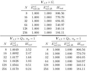
Table 2. Approximation errors for Solution (7.2), on meshes with λ= 10−4. Errors using the inf-sup stable pair V1,P×G(top table). Errors using V1,P×QP, αp = 1, with sv given by (6.3) (bottom left) and (6.1) (bottom right).

V1,P×G, N E_nat,rel _2a E_nat,rel_2b IEnat

8 1.000 1.000 806.56 16 1.000 1.000 770.70 32 1.000 1.000 694.05 64 1.000 1.000 540.97 128 1.000 1.000 340.14 256 1.000 1.000 184.11

V1,P×QP,αp= 1 N E_nat,rel₃ IEnat

8 1.0049 3.52 16 1.0092 2.47 32 1.0177 1.68 64 1.0426 1.03 128 1.0564 0.51 256 1.0170 0.24

V1,P×QP,αp = 1 N E_nat,rel_2a E_nat,rel _2b IEnat

8 1.000 1.000 806.56 16 1.000 1.000 770.70 32 1.000 1.000 694.05 64 1.000 1.000 540.97 128 1.000 1.000 340.14 256 1.000 1.000 184.11

is much stronger for the case in which sv is given by (6.1) (for both definitions of the stabilisation parameter) than for the case ofsv given by (6.3).

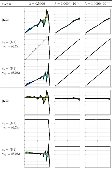
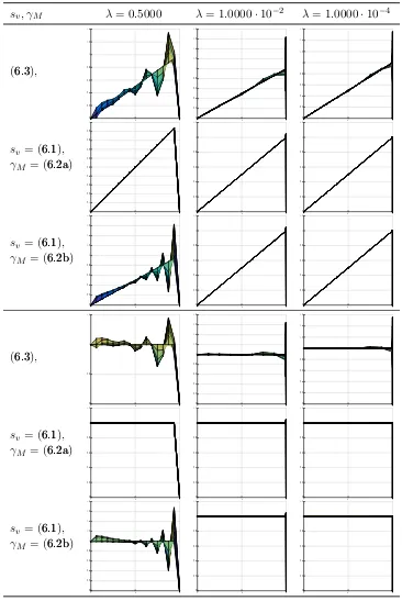
We next try to assess the importance of the last point made in the last paragraph. For this, we plot the velocity profiles obtained by the different methods in in Figures 7– 8. We note that the stabilisation term sv given by (6.1) produces a profile which is smoother, especially when (6.2a) is used, producing a discrete velocity which is almost free of oscillations, whereas the profile obtained from the method usingsv given by (6.3) presents large oscillations. This is in accordance with our earlier claim that the norm induced by (6.1) is stronger than the one induced by (6.3). Furthermore, from Figures 7– 8 we see that the different definitions of the stabilisation parameters give different results on shape regular meshes (see the results for λ= 1/2). However, on anisotropic meshes the behaviour is similar and oscillations and overshoots are significantly reduced.

sv, γM λ= 0.5000 λ= 1.0000·10−2 λ= 1.0000·10−4 (6.3), 0 0.2 0.4 0.6 0.8 1 1.2 1.4 0 y 1 0 0.2 0.4 0.6 0.8 1 1.2 1.4 1.6 0 y 1 0 0.2 0.4 0.6 0.8 1 1.2 1.4 1.6 0 y 1

sv = (6.1), γM = (6.2a)

0 0.1 0.2 0.3 0.4 0.5 0.6 0.7 0.8 0.9 1 0 y 1 0 0.2 0.4 0.6 0.8 1 1.2 0 y 1 0 0.2 0.4 0.6 0.8 1 1.2 0 y 1

sv = (6.1), γM = (6.2b)

0 0.2 0.4 0.6 0.8 1 1.2 1.4 1.6 1.8 0 y 1 0 0.2 0.4 0.6 0.8 1 1.2 0 y 1 0 0.2 0.4 0.6 0.8 1 1.2 0 y 1 (6.3), 0 0.5 1 1.5 0 y 1 0 0.2 0.4 0.6 0.8 1 1.2 1.4 1.6 0 y 1 0 0.2 0.4 0.6 0.8 1 1.2 1.4 1.6 0 y 1

sv = (6.1), γM = (6.2a)

0 0.2 0.4 0.6 0.8 1 1.2 0 y 1 0 0.2 0.4 0.6 0.8 1 1.2 0 y 1 0 0.2 0.4 0.6 0.8 1 1.2 0 y 1

sv = (6.1), γM = (6.2b)

0 0.2 0.4 0.6 0.8 1 1.2 1.4 1.6 1.8 0 y 1 0 0.2 0.4 0.6 0.8 1 1.2 0 y 1 0 0.2 0.4 0.6 0.8 1 1.2 0 y 1

sv, γM λ= 0.5000 λ= 1.0000·10−2 λ= 1.0000·10−4 (6.3), 0 0.2 0.4 0.6 0.8 1 1.2 1.4 0 y 1 0 0.2 0.4 0.6 0.8 1 1.2 1.4 1.6 1.8 0 y 1 0 0.2 0.4 0.6 0.8 1 1.2 1.4 1.6 0 y 1

sv = (6.1), γM = (6.2a)

0 0.1 0.2 0.3 0.4 0.5 0.6 0.7 0.8 0.9 1 0 y 1 0 0.2 0.4 0.6 0.8 1 1.2 0 y 1 0 0.2 0.4 0.6 0.8 1 1.2 0 y 1

sv = (6.1), γM = (6.2b)

0 0.2 0.4 0.6 0.8 1 1.2 1.4 1.6 1.8 0 y 1 0 0.2 0.4 0.6 0.8 1 1.2 0 y 1 0 0.2 0.4 0.6 0.8 1 1.2 0 y 1 (6.3), 0 0.5 1 1.5 0 y 1 0 0.2 0.4 0.6 0.8 1 1.2 1.4 1.6 1.8 0 y 1 0 0.2 0.4 0.6 0.8 1 1.2 1.4 1.6 0 y 1

sv = (6.1), γM = (6.2a)

0 0.2 0.4 0.6 0.8 1 1.2 0 y 1 0 0.2 0.4 0.6 0.8 1 1.2 0 y 1 0 0.2 0.4 0.6 0.8 1 1.2 0 y 1

sv = (6.1), γM = (6.2b)

0 0.2 0.4 0.6 0.8 1 1.2 1.4 1.6 1.8 0 y 1 0 0.2 0.4 0.6 0.8 1 1.2 0 y 1 0 0.2 0.4 0.6 0.8 1 1.2 0 y 1

0 y

1 0 0.2 0.4 0.6 0.8 1 1.2 1.4

0 y

1 0 0.2 0.4 0.6 0.8 1

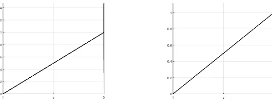
Fig. 9 Discrete velocities for Example 1 on a mesh with N= 8, λ= 10−3. The method uses V1,P×QP, sp, andαp = 1, and the ”reduced” stabilised method (i.e., (6.1) where the fluctuation of the convective derivative has been removed, depicted on the left), and the full stabilising term (6.1), depicted on the right.

8 Conclusion

In this work we have generalised the results from [ABW15, LS13] to the lowest order pair Q21 ×P0 in partitions that contain refined corner patches, and extended this gen-eralisation to the Oseen equation. To analyse the resulting methods we have used, and adapted when necessary, the abstract approach given in [MT15]. This allowed us to present stability and convergence results that are valid both in the inf-sup stable and stabilised cases. A precise definition, by means of a weighted grad-div term enhanced by a penalisation of the convective derivative, of the stabilisation term for the veloc-ity has been proposed, justified, and tested numerically. This new definition seems to outperform some previously known alternatives, at least numerically. This study leaves, nevertheless, some open questions such as the extension of this idea to graded meshes, more general quadrilaterals, and the three-dimensional case. For the latter, the detailed stability analysis of the underliningV1,P×QPspace needs to be done. These will be the

topics of future research.

Acknowledgement

AW wants to acknowledge the partial support given by the Asociaci´on Mexicana de Cultura A.C.. The authors want to thank Jen Pestana for helpful discussions related to discrete inf-sup constants. The authors also want to thank the anonimous referees for their careful reading of the paper and their useful suggestions.

9 Appendix

In this appendix we detail a local trace inequality. Its proof does not seem to be available, and that is why we present it here.

Lemma 9.1. Let K be a parallelogram, let e be one of its edges, and let ti be a unit

tangential vector of an edge ei that is incident to e. Then, for all v ∈ H1(K) the

following holds

kv_k2_{0,e ≤} |e|

|K|kvk0,K

kv_k0,K + 2_|ei| kti· ∇vk_0,K

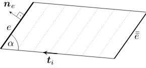
Proof. Let v∈H1(K). Using the notation given by Figure 10, we define

φ_e(x) := ne·(x−p¯¯e)

ti,

wherene is the outer unit normal to edgee andpe¯¯is any point on the opposite edge ¯e¯ (parallel to e). Since φ_e∈C∞(K), the following Green’s formula holds

Z

∂K

(φ_e·n)v2ds=

Z

K

v2divφ_edx+ 2

Z

K

v(φ_e· ∇v) dx. (9.2)

We now evaluate the terms involvingφ_e. We start by observing that

divφ_e=ne1ti1+ne2ti2 =ne·ti = cos(π−(π/2 +α)) = sin(α). (9.3) Furthermore, the unit tangential and normal vector of edge eform a basis of R2, that

is, eachx_∈K is representable as x=pe¯¯+r1(x)|e|−1|K|ne+r2(x)te with r1 ∈[0,1] and r2 ∈R. Therefore, the definition ofφe simplifies to

φ_e=r1(x)|e|−1|K|ti for r1 ∈[0,1], (9.4) withr1≡0 on ¯¯eandr1≡1 one(sinceK is a parallelogram). Therefore,φe·n= 0 on ∂K\eand

Z

∂K

(φ_e·n)v2ds=

Z

e

(φ_e·ne)v2ds= | K_|

|e|(ne·ti)

Z

e

v2ds= |K|

|e| sin(α)

Z

e

v2ds . (9.5)

Then, inserting (9.3), (9.4) and (9.5) into (9.2) we arrive at

sin(α)|K|

|e_|

Z

e

v2ds= sin(α)

Z

K

v2dx+|K|

|e_|

Z

K

r1(x)2v(ti· ∇v) dx.

After recalling maxx_∈Kr1(x) = 1 and applying Cauchy–Schwarz’s inequality the last identity gives

kvk20,e ≤ kvk0,K

|e|

|K|kvk0,K +

2

sin (α)kti· ∇vk0,K

= |e|

|K|kvk0,K

kv_k0,K+ 2_|ei| kti· ∇vk0,K

,

which finishes the proof.

We now prove a result that allows us to compute the inf-sup constant of the Oseen problem. We have not been able to locate this exact result in the literature, and that is why we detail its proof here.

e

ne

α ¯¯e

ti

Lemma 9.2. Let A, B ∈ Rn×n and let B be symmetric positive definite. Then, the inf-sup constant σ defined by

σ= min z∈Rn

max ξ∈Rn

ξT_Az

kξkBkzkB

is given by the smallest singular value of Ae := L−TAL−1 where L is defined by the

Cholesky decomposition B =LTL.

Proof. First, a direct application of Theorem 2 in [CF03] implies

σ_ky_{k2 ≤}max x∈Rn

xT

e

Ay

kxk2

for all y_∈Rn,

whereσ is the smallest singular value ofAe. Then, changing variables (x=Lξ, y=Lz)

we get

σ_kLz_{k2 ≤}max ξ∈Rn

(Lξ)TL−TAL−1(Lz)

kLξ_k2 = maxξ∈Rn

ξTAz

kLξ_k2 for all z∈R n_.

Finally, realising_kz_k2_B =_hBz, z_i=

LT_{Lz, z}

=_hLz, Lz_i=_kLz_k2₂ finishes the proof.

References

[ABV06] R. Araya, G. R. Barrenechea, and F. Valentin,Stabilized finite element meth-ods based on multiscale enrichment for the Stokes problem, SIAM Journal on Numerical Analysis 44, (2006), no. 1, 322-348.

[ABW15] M. Ainsworth, G. R. Barrenechea, and A. Wachtel, Stabilization of high as-pect ratio mixed finite elements for incompressible flow, SIAM Journal on Numerical Analysis 53(2015), no. 2, 1107–1120.

[AC00] M. Ainsworth and P. Coggins,The stability of mixedhp-finite element methods for Stokes flow on high aspect ratio elements, SIAM J. Numer. Anal.38(2000), no. 5, 1721–1761.

[AKL08] T. Apel, T. Knopp, and G. Lube, Stabilized finite element methods with anisotropic mesh refinement for the Oseen problem, Appl. Numer. Math. 58

(2008), no. 12, 1830–1843.

[BB01] R. Becker and M. Braack,A finite element pressure gradient stabilization for the Stokes equations based on local projections, Calcolo38(2001), no. 4, 173– 199.

[BBF93] C. Baiocchi, F. Brezzi, and L.P. Franca, Virtual bubbles and Galerkin-least-squares methods (Ga.L.S.), Comput. Methods Appl. Mech. Engrg., 105, (1993), no. 1, 125-141.

[BB+07] M. Braack, E. Burman, V. John, and G. Lube,Stabilized finite element meth-ods for the generalized Oseen problem, Comput. Methods Appl. Mech. Engrg.

196 (2007), no. 4-6, 853–866.

[BDG06] P. B. Bochev, C. R. Dohrmann, and M. D. Gunzburger, Stabilization of low-order mixed finite elements for the Stokes equations, SIAM J. Numer. Anal.

44 (2006), no. 1, 82–101.

[BF01] F. Brezzi and M. Fortin, A minimal stabilisation procedure for mixed finite element methods, Numer. Math. 89(2001), no. 3, 457–491.

[BH82] A. N. Brooks and T. J. R. Hughes, Streamline upwind/Petrov-Galerkin for-mulations for convection dominated flows with particular emphasis on the in-compressible Navier-Stokes equations, Comput. Methods Appl. Mech. Engrg.

32 (1982), no. 1-3, 199–259.

[Bla08] J. Blasco, An anisotropic GLS-stabilized finite element method for incom-pressible flow problems, Comput. Methods Appl. Mech. Engrg. 197 (2008), no. 45-48, 3712–3723.

[BLR12] M. Braack, G. Lube, and L. R¨ohe, Divergence preserving interpolation on anisotropic quadrilateral meshes, Comput. Methods Appl. Math. 12 (2012), no. 2, 123–138.

[Bra08] M. Braack,A stabilized finite element scheme for the Navier-Stokes equations on quadrilateral anisotropic meshes, M2AN Math. Model. Numer. Anal. 42

(2008), no. 6, 903–924.

[Bur08] E. Burman, Pressure projection stabilizations for Galerkin approximations of Stokes’ and Darcy’s problem, Numerical Methods for Partial Differential Equations 24(2008), no. 1, 127–143.

[BV10] G. R. Barrenechea, and F. Valentin, A residual local projection for the Oseen equation, Comput. Methods Appl. Mech. Engrg. 199, (2010), 1906-1921.

[BW15] G. R. Barrenechea and A. Wachtel, A note on the stabilised Q1-P0 method on quadrilaterals with high aspect ratios, Boundary and Interior Layers, Pro-ceedings of BAIL 2014, P. Knobloch (Ed.), Lecture Notes in Computational Science and Engineering, Vol. 108, (2015), pp. 1-11.

[Cod08] R. Codina, Analysis of a stabilized finite element approximation of the Os-een equations using orthogonal subscales, Applied Numerical Mathematics58, (2008), 264-283.

[CF03] Z.-H. Cao and L.-H. Feng, A note on variational Representation for singular values of matrix, Applied Mathematics and Computation, 143, (2003), 559-563.

[FF92] L. P. Franca and S. Frey,, Stabilized finite element methods. II. The incom-pressible Navier-Stokes equation, Comput. Methods Appl. Mech. Engrg. 99

[FH88] L. P. Franca, and T. J. R. Hughes,Two classes of mixed finite element meth-ods, Comput. Methods Appl. Mech. Engrg. 69(1988), no. 1, 89-129.

[GL+12] K. Galvin, A. Linke, L. Rebholtz, and N. Wilson,Stabilizing poor mass conser-vation in incompressible flow problems with large irrotational forcing and ap-plication to thermal convection, Comput. Methods Appl. Mech. Engrg.,237, (2012), 166-176.

[GR86] V. Girault and P.-A. Raviart,Finite element methods for Navier Stokes equa-tions, Springer, Berlin, 1986.

[HFB86] T. J. R. Hughes, L. P. Franca, and M. Balestra,A new finite element formula-tion for computaformula-tional fluid dynamics. V. Circumventing the Babuˇska-Brezzi condition: a stable Petrov-Galerkin formulation of the Stokes problem accom-modating equal-order interpolations, Comput. Methods Appl. Mech. Engrg.

59 (1986), no. 1, 85–99.

[HFH89] T. J. R. Hughes, L. P. Franca, and G. Hulbert, A new finite element for-mulation for computational fluid dynamics. VIII. The Galerkin/least-squares method for advective-diffusive equations, Comput. Methods Appl. Mech. En-grg. 73(1989), no. 2, 173-189.

[Joh17] V. John, Finite element methods for incompressible flow problems, Springer Series in Computational Mathematics, vol. 51, Springer-Verlag, 2017.

[JJ+14] E. W. Jenkins, V. John, A. Linke, and L. G. Rebholz, On the parameter choice in grad-div stabilization for the Stokes equations, Adv. Comput. Math.

40 (2014), no. 2, 491–516.

[Kno10] P. Knobloch, A generalization of the local projection stabilization for convection-diffusion-reaction equations, SIAM J. Numer. Anal. 48 (2010), no. 2, 659–680.

[KS92] N. Kechkar and D. J. Silvester, Analysis of locally stabilized mixed finite ele-ment methods for the Stokes problem, Math. Comp. 58(1992), no. 197, 1–10.

[LM+09] W. Layton, C. Manica, M. Neda, M.A. Olshanskii, and L. Rebholtz, On the accuracy of the rotation form in simulations of the Navier-Stokes equations, Journal of Computational Physics. 228 (2009), no. 9, 3433-3447.

[LS13] Q. Liao and D. Silvester, Robust stabilized Stokes approximation methods for highly stretched grids, IMA J. Numer. Anal. 33(2013), no. 2, 413–431.

[MPP03] S. Micheletti, S. Perotto, and M. Picasso, Stabilized finite elements on anisotropic meshes: a priori error estimates for the advection-diffusion and the Stokes problems, SIAM J. Numer. Anal. 41(2003), no. 3, 1131–1162.

[MT15] G. Matthies and L. Tobiska, Local projection type stabilization applied to inf-sup stable discretizations of the Oseen problem, IMA J. Numer. Anal. 35

(2015), no. 1, 239–269.

[OR04] M.A. Olshanskii, and A. Reusken, Grad-div stabilization of the Stokes equa-tions, Mathematics of Computation,73, (2004), 1699- 1718.

[PS85] J. Pitk¨aranta and T. Saarinen,A multigrid version of a simple finite element method for the Stokes problem, Math. Comp. 45(1985), no. 171, 1–14.