Date of publication xxxx 00, 0000, date of current version xxxx 00, 0000.
Digital Object Identifier 10.1109/ACCESS.2017.Doi Number
Uncertainty-aware dynamic reliability analysis
framework for complex systems
Sohag Kabir1, Mohammad Yazdi2, Jose Ignacio Aizpurua3, and Yiannis Papadopoulos1 1School of Engineering and Computer Science, University of Hull, UK
2Centre for Marine Technology and Ocean Engineering (CENTEC), University of Lisbon, Portugal 3Department of Electronic and Electrical Engineering, University of Strathclyde, UK
Corresponding author: Sohag Kabir (e-mail: [email protected]).
This work was partly funded by the DEIS H2020 project (Grant Agreement 732242).
ABSTRACT Critical technological systems exhibit complex dynamic characteristics such as time-dependent behaviour, functional dependencies among events, sequencing and priority of causes that may alter the effects of failure. Dynamic fault trees (DFTs) have been used in the past to model the failure logic of such systems, but the quantitative analysis of DFTs has assumed the existence of precise failure data and statistical independence among events, which are unrealistic assumptions. In this paper, we propose an improved approach to reliability analysis of dynamic systems, allowing for uncertain failure data and statistical and stochastic dependencies among events. In the proposed framework, DFTs are used for dynamic failure modelling. Quantitative evaluation of DFTs is performed by converting them into generalised stochastic Petri nets. When failure data are unavailable, expert judgment and fuzzy set theory are used to obtain reasonable estimates. The approach is demonstrated on a simplified model of a Cardiac Assist System.
INDEX TERMS Dynamic systems, Fault tree analysis, Fuzzy set theory, Petri nets, Reliability analysis.
I. INTRODUCTION
Fault tree analysis (FTA) is widely used for safety and reliability analysis of systems. FTA models are well-structured and easily understood. However, they are unable to model some aspects of system behaviour such as dependencies between subsystems and components, and ordering among the component failure occurrences. For this reason, application of classical FTA is limited to systems whose components have no stochastic and temporal dependencies. However, in practical technological systems, not all events are statistically independent, and in such situations, the assumption of statistical and stochastic independence of events can lead to an inappropriate estimation of system reliability. In order to model dependencies among events, classical FTA has been extended to introduce dynamic fault trees [1] and temporal fault trees (TFTs) [2], [3].
DFTs is a well-established dynamic version of the Fault Tree (FT) that enables modelling time-dependent behaviour in dynamic systems. Temporal dependencies among the system components and ordering among events are modelled using DFT gates such as functional dependency (FDEP), Priority-AND (PPriority-AND), and SPARE gates. These gates capture temporal behaviour, and therefore classical combinatorial
solutions for the quantification of FTs are not suitable for DFTs. Alternative analytical solutions have been proposed in [4], [5], but these approaches do not account for stochastic dependencies among events or cater for uncertainty in failure data.
DFTs can be quantified by converting them into Markov chains [6], [7]. However, Markov chains are limited to exponential distributions and the associated memoryless property. This requirement may be too tight for modelling
complex systems. Bayesian networks (BN) based
Generalised Stochastic Petri Nets (GSPNs) [12] are also used to quantify DFTs. The underlying reachability graph of a GSPN is isomorphic to a continuous time Markov chain. However, in contrast to Markov chains, GSPN models are able to model non-exponential distributions. Similar to BN-based models, GSPN can model stochastic dependencies among events. In fact, Generalised Continuous time BN (GCTBN) models [13] are solved by converting them to GSPN. In addition to the benefits of BN-based models for DFT modelling, GSPN models provide a one-to-one interface for other purposes such as formal specification and verification, which cannot be handled with other formalisms. Accordingly, this work adopts GSPN as an underlying stochastic modelling formalism to quantify and evaluate DFT models.
Generally, quantitative FTA assumes known failure rates or probabilities of failure of system components. In practice, it is often difficult to obtain this data for all the components, which introduces uncertainty in the analysis. A few methods have been proposed to perform quantitative analysis with unknown and uncertain failure data. One of such approaches is the fuzzy fault tree analysis (FFTA) [14], which is an extension to classical fault trees where fuzzy failure data are used in the reliability quantification process instead of crisp values. More information about FFTA and its applications in different areas can be found in [15]. As FFTA is an extension to classical FTs, it inherits all the limitations of the classical FTA.
Recently, some attempts such as [16]–[23] have been made to incorporate the concept of uncertainty in DFT analysis. In this paper, we propose a comprehensive uncertainty-aware framework for reliability analysis of complex dynamic systems. The framework combines DFTs with GSPN and fuzzy set theory. DFTs are used to model the dynamic failure behaviour of systems. To quantify the DFTs including statistical and stochastic dependencies, DFTs are translated into a GSPN model. Fuzzy set theory and expert judgments are combined together to obtain estimates of failure data for basic events (BEs) of the DFT when such data are unavailable. Accordingly, the contribution of this paper is the proposal of a novel method, which is able to take into account statistical and temporal dependencies in the failure logic as well as uncertainty modelling in component failure data. This approach quantifies complex and dynamic systems accurately taking into account temporal and stochastic dependencies, and it enables the reliability analysis of complex systems with lack of exact failure data of its constituent components.
The rest of this paper is organised as follows. Section II presents fundamental concepts and related work. Section III introduces the proposed reliability analysis framework. Section IV applies the proposed approach to a numerical case study and finally, Section V draws conclusions.
II. BACKGROUND AND RELATED WORKS
A. DYNAMIC FAULT TREE ANALYSIS
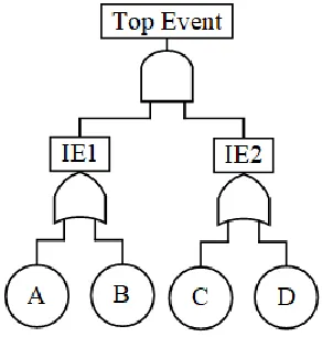
[image:2.576.345.491.192.345.2]Fault tree analysis was first introduced by Bell laboratories in 1962 for a ballistic control system [24]. The process to design an FTA model follows a top-down procedure, starting from the undesired system level top-event (TE), which represents the system failure condition. The TE is decomposed into a combination of intermediate events, which are defined with Boolean logic. The intermediate events are further decomposed by using Boolean logic down to the specification of the lowest-level event causes, which are named Basic Events (BEs). Fig. 1 shows an FTA example.
FIGURE 1. Example fault tree.
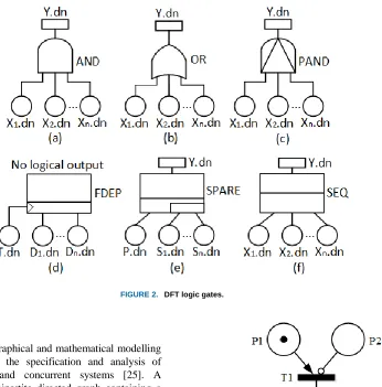
FTA cannot accommodate temporal dependencies. For instance, Boolean logic does not allow temporal ordering of events the effect of which may be significant. For instance, many systems use activation mechanisms to activate spares when primary systems fail. Whether the activation mechanism has failed before or after failure of the primary defines whether the spare is activated. To address such issues, classical FTA was augmented with gates that capture dynamics in the DFT method [1]. Fig. 2 below shows the main static and dynamic gates used in DFT analysis, the function of which is briefly defined as follows:
Y = AND (X1, …, XN), Y occurs only if all the BEs
{X1, …, XN} fail simultaneously.
Y = OR (X1, …, XN), Y occurs if any of the BEs {X1,
…, XN} fails.
Y = PAND (X1, …, XN), Y occurs only if BEs {X1,
…, XN} fail in left-to-right graphical order. That is,
let us denote before with the symbol “<”, then PAND is defined as: Y = AND (X1<X2, …, XN-1<XN). FDEP (T, D1, …, DN): the occurrence of the trigger
event T enforces the occurrence of the BEs {D1, …,
DN}. This gate has no logical output.
Y = SPARE (P, S1, …, SN), the primary input P is an
active BE, while the standby inputs {S1, …, SN} are
Y = SEQ (X1, …, XN) models the sequence
enforcing event, which enforces the events to occur in an specific left-to-right order.
A DFT model can be analysed qualitatively and quantitatively. The main result of qualitative analysis is the Minimal Cut Sequence Set (MCSQ) expression, which determines which are the temporal combination of minimal necessary BEs that can cause the system-level failure. The main outcome of quantitative analysis is the failure probability of the top event (TE), typically representing the probability of a system failure. The work presented in this paper focuses on quantitative analysis.
[image:3.576.132.478.221.572.2]Quantitative analysis requires specification of probabilistic distributions of BEs. Widely accepted distributions include Weibull and exponential distributions, but this is dependent on the specific system under study. Note that the quantitative analysis is not only limited to the system level failure probability, other assessments and metrics can be extracted from the DFT model such as the criticality analysis, which calculates the contribution of each BE to the occurrence of the TE.
FIGURE 2. DFT logic gates.
B. PETRI NETS
Petri nets (PNs) are a graphical and mathematical modelling formalism suitable for the specification and analysis of complex, distributed and concurrent systems [25]. A conventional PN is a bipartite directed graph containing a finite set of places, a finite set of transitions, and a finite set of directed arcs. In a PN model, places and transitions are graphically represented by circles and rectangles, respectively. Directed arcs are used to connect places to transitions and transitions to places. Tokens (black dots) are used to specify the states of the places in a PN model. The enabling condition of a transition is defined as the presence of a certain number of tokens in its input place(s). When a transition fires, a certain number of tokens are deposited to the output place(s) of the transition.
FIGURE 3. Example of a PN.
has no token and it disables a transition when a place has a token, i.e., opposite behaviour of the normal arc. Stochastic Petri nets (SPNs) [26] are another extension of PNs that allow defining exponentially distributed transition delays. GSPNs [13] extended SPNs by allowing inclusion of immediate and timed transitions in a single PN model. Black and white bars are used to represent immediate and timed transitions, respectively. In a GSPN model, an immediate transition has priority over a timed transition and fires first when both are enabled to fire simultaneously.
Application of PNs for system safety and reliability analysis can be traced back to 1980s [27], [28]. In [29], [30] methodologies have been proposed to convert classical fault trees to PNs for reliability evaluation. DFTs have been translated into GSPNs for reliability analysis of dynamic systems in [31]–[33].
C. FUZZY SETS IN UNCERTAINTY ANALYSIS
The fuzzy set theory was formalized in 1965 by Zadeh [34], and also has been widely applied, including for dealing with uncertainty in safety and reliability analysis. The use of qualitative fuzzy terms indeed provides flexible modelling of imprecise data and information. The main purpose of fuzzy terms is to assist gradual transition between varieties of conditions. A classical set contains expressions, which satisfy exact characteristics of membership. On the other hand, a fuzzy set contains expressions that satisfy ambiguous characteristics of membership, i.e. the characteristics of fuzzy set expressions can be partial. A comparison between a classical set (Boolean) and a fuzzy set can be seen in Fig. 4. As it can be seen for classical sets, in a universe U, an element D can either be a member of some crisp set S or not. This binary characteristic of membership can be defined as follows:
US= {
1 when D ∈ S ( D is a member of S)
[image:4.576.43.274.522.611.2]0 when D ∉ S (D is not a member of S) (1)
FIGURE 4. Diagrams for a classical set (Boolean) and a fuzzy set [35]. The characteristic of the binary membership is extended by Zadeh to incorporate the different rate of membership on the real continuous distance interval from zero to one [0, 1]. Zero means that there is no membership whereas the endpoint of the distance (one) indicates complete membership. A set of universe U, which accommodates rates of membership is named a fuzzy set. Thus, using the mathematical notation
μS̃ (D) ϵ [0,1], a fuzzy set S̃ can be defined with μS̃ (D) the rate of membership of element D in S̃, or briefly membership of S̃. The value of μS̃ (D) belongs in the distance interval [0, 1] and corresponds to the rate to which element D is a member of fuzzy set S̃. The higher the value of μS̃ (D) the stronger the rate of membership of D in S̃. Information about arithmetic operations on fuzzy numbers can be found in [36].
Several developments of fuzzy set theory have been proposed to improve the flexibility of conventional fuzzy set theory. Atanassov [37] introduced an extension of fuzzy set theory called intuitionistic fuzzy sets. These include membership as well as non-membership functions, and can deal better with uncertainties that may happen from biased results. However, intuitionistic fuzzy sets increase complexity and computation time. Chen and Hwang developed fuzzy reasoning using algebraic properties of fuzzy sets in order to provide a solution to complex problems, including bounded-sum, unbounded-bounded-sum, union, intersection, and algebraic product [38]. In addition, Atanassov [39] introduced an extension to intuitionistic fuzzy sets with hesitation margin groups to cope with complexity. However, computation time remains a significant limitation of this model.
III. THE PROPOSED UNCERTAINTY-AWARE DYNAMIC RELIABILITY APPROACH
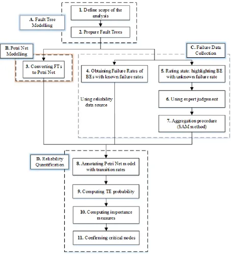
The framework of the proposed approach is shown in Fig. 5. The approach consists of four steps: Fault Tree Modelling, Petri Net Modelling, Failure Data Collection, and Reliability Quantification. Fault Tree Modelling deals with the creation of a DFT of the system under study. Petri Net Modelling and Failure Data Collection are executed in parallel, where in the Petri Net Modelling step the DFT is mapped into a GSPN model and in the Failure Data Collection step the failure rate of BEs with unknown data are collected. These data are then incorporated into the GSPN model. The final step is the Reliability Quantification, where all the analyses are performed on the GSPN model. Detailed descriptions of the steps are provided in the following subsections.
A. FAULT TREE MODELLING
In this step, the dynamic behaviour of systems is modelled using DFT. As DFT is an extended version of classical fault trees, it can be created following the procedure described in the fault tree handbook [40]. The objectives of a DFT in general include (1) identifying all possible ways of causing an undesired event which is called top event (TE), (2) providing a provable record of the analysis process, and (3) providing the foundations of design evaluation and practical alternatives [41].
analysis and which are not. Finally, the resolution is determined defining the level of detail in the analysis of root causes. DFTs are constructed in a top-down fashion using the
[image:5.576.55.526.116.635.2]logic gates outlined in section II.A to show the logical and temporal connections between events. The following sections deal with DFT evaluation.
FIGURE 5. Framework of the proposed uncertainty-aware approach.
B. PETRI NET MODELLING
This step takes the DFT generated in the previous step as input and converts it into a GSPN model. Εach DFT module (e.g., basic event, logic gate) is translated into a GSPN sub-net and all the sub-nets are combined to obtain an overall GSPN of the
(𝜆) is exponentially distributed, then the probability that the transition is fired at the time instant 𝑡 is 1 − 𝑒−𝜆𝑡 . The place x.dn represents the failed state of the basic event x. This place receives token when x.f fires. Note that the failure rate of some BEs may not be available. The GSPN of such events would still be created, but the value of the firing rate of the timed transition is left empty, and incorporated later on using expert judgment.
[image:6.576.292.535.245.565.2]FIGURE 6. GSPN of a basic event.
FIGURE 7. GSPN of AND gate.
FIGURE 8. GSPN of OR gate.
GSPN of Boolean gates (AND and OR) are shown in Figs. 7 and 8, respectively. In the GSPN model of the AND gate, all input places (X1.dn, X2.dn,…, Xn.dn) are connected to a single
immediate transition. When all the input places get a token, then the immediate transition fires and deposits a token to the output place, X.dn, i.e. all inputs of the AND gate must be true to make the outcome of the AND gate true. Unlike the GSPN model of the AND gate, the GSPN model of the OR gate represents disjunction of events. In the latter, each of the input
places is connected to distinct immediate transition, which makes sure that the output place will get a token when any of the place gets a token, i.e., the output of the OR gate becomes true when any of the inputs becomes true.
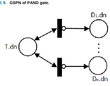
In the GSPN model of the PAND gate, the place X.dn represents the outcome of the PAND gate. If events occur in a required sequence, then this place gets a token. If the sequencing is violated, then the place X.ok gets a token, a confirmation that PAND gate output cannot be true. This place is connected to the immediate transition Tn using an inhibitor
arc, which ensures that the place representing the PAND gate outcome will not get a token if all the input events of the PAND gate occur but not in the required sequence.
FIGURE 9. GSPN of PAND gate.
FIGURE 10. GSPN of FDEP gate.
The GSPN model in Fig.10 models the behaviour of the FDEP gate. As seen in section II.A, the FDEP gate has no logical output. If the trigger event occurs, the dependent event will also occur. In the GSPN model, the place T.dn represents the failed state of the trigger event, whereas the places {D1.dn,
…, Dn.dn} represent the failed state of the dependent events.
[image:6.576.321.511.411.559.2]token, i.e., dependent events will occur if the trigger event occurs.
FIGURE 11. GSPN of SPARE gate.
FIGURE 12. GSPN of SEQ gate.
The GSPN model of a warm spare gate is shown in Fig. 11. The places S1.dn and S2.dn represent the failed state of the two spare components S1 and S2, respectively. For both components, it is possible to reach the failed state in two ways. In the first way, when the components are in passive mode, the internal failure of the components will take them to failed states. In the GSPN model, S1.passive and S2.passive represent the passive modes of the two spare components. Timed transitions S1.p_f and S2.p_f are two timed transitions representing the failure rate of the components in passive mode. Firing of these transitions will take the components to
their failed mode. In the second way, firstly, the spare components are activated due to the failure of the primary component. This scenario is modelled by immediate transitions wsp1 and wsp2 for components S1 and S2, respectively. Timed transitions S1.a_f and S2.a_f are two timed transitions representing the failure rate of the components in their active mode and firing of these transitions will take the components from their active mode to their failed mode. When places P.dn, S1.dn and S2.dn get marked (i.e., all components failed), the immediate transition wsp3 will fire and deposit a token to place Y.dn, i.e., making the outcome of the spare gate true. A cold spare gate can be modelled using GSPN in the similar way; however, for the cold spare gate the part showing the failure of the spare components in passive mode will not be required.
A GSPN model of a SEQ gate is shown in Fig. 12. This model forces the input events to occur in a sequence. For instance, if we consider timed transition X2.f, this can fire only
after X1.dn gets a token, i.e., when the event X1 occurs. In this
way, the GSPN model ensures that the event X2 can occur only
after X1. The place X.dn represents the outcome of the SEQ
gate and this place will get a token when the last event in the SEQ gate becomes true thus maintaining the sequencing.
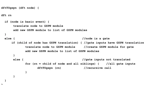
Given the above conversion rules for the basic event and the logic gates, Fig.13 shows a pseudocode of a function that converts a DFT to GSPN in the course of a depth first traversal of the DFT. We assume a typical computational representation of a tree, where a gate is a ‘node’ pointing to a ‘child’ (first input to the gate) which is then linked to a list of siblings representing the rest of gate inputs. Basic events do not have a child and can be detected as such.
[image:7.576.42.278.99.266.2]C. FAILURE DATA COLLECTION
The BEs of the DFT can be classed into those with known failure rates and those with unknown failure rates. Known failure rates are typically determined by consulting reliability data handbooks such as PDS or OREDA [45],[46]. For estimation of unknown failure rates, methods include statistical extrapolation, and expert judgment [47]. In this study, the expert judgment method is used as an integration of fuzzy set theory and subjective opinions [48]. Various methods are available to aggregate experts’ opinion, such as fuzzy priority relations, game theory, arithmetic averaging operation, max–min Delphi method, and similarity aggregation method (SAM) [49],[50],[51]. Liu et al. [52] have argued that there is no way to determine which technique is superior.
In this study, we have opted for the SAM method, which considers both homogeneous and heterogeneous groups of experts. The qualitative terms used in the study to express and collect the experts’ opinions are defined as a combination of fuzzy triangular and fuzzy trapezoidal numbers from which failure rates are estimated [53]. The group of experts was defined as heterogeneous because in practice their opinion brings different value and weight to the final result. Consequently, for qualifying the measurements, the relevance of the experts was ranked using a methodology that takes into account the professional position, job experience, education
level, and age (see [54]-[59]). The score rating of the experts was determined according to Table I.
The rating of an expert judgment can be done according to the weight given to each BE. The concept of linguistic expressions has a high value in dealing with any circumstances that are ill-defined or complex to be described in the old model of quantitative expression [24]. In order to convert qualitative terms to corresponding fuzzy numbers, Chen and Hwang [38] represented a numerical approximation. To acquire this criterion, there are common verbal expressions in the system. Chen’s conversion scale is provided in Table II in which scale one contains two verbal terms and scale eight contains thirteen verbal terms [60], [61]. In addition, Lavasani et al. [58] suggested that humans are capable of distinguishing effectively between five and nine linguistic expressions that cover a range of possible outcomes. Using this theory, we have opted for a scale of six using five verbal terms that provide options for the subjective evaluation of experts with regards to estimating the probability of failure. Table III presents the fuzzy membership function in the form of trapezoidal numbers.
The linguistic expressions of Fig. 14 are in the form of both triangular and trapezoidal fuzzy numbers and it is possible to transform all the triangular fuzzy numbers to the corresponding trapezoidal fuzzy numbers. Table III illustrates the fuzzy numbers of Fig. 14 in the form of trapezoidal numbers.
dftTOgspn (dft node) {
dft rn
if (node is basic event) {
translate node to GSPN module
add new GSPN module to list of GSPN modules }
else { //node is a gate
if (child of node has GSPN translation) { //gate inputs have GSPN translations translate node to GSPN module //create GSPN module for gate
add new GSPN module to list of GSPN modules }
else { //gate inputs not translated for (rn = child of node and all siblings) { //all gate inputs dftTOgspn (rn) //recursive call
} }
[image:8.576.32.534.47.345.2]} }
FIGURE 14. Transformation of scale six.
Let us assume that each expert, El (l = 1, 2, . . ., m) expresses
their viewpoint about a specific attribute in a certain context using qualitative terms. The qualitative terms are converted to the corresponding fuzzy numbers as follows:
TABLEI.SCORE RATING ACCORDING TO THE EXPERT’S TRAITS
Condition Classification Score
Professional position
Senior academic, GM/DGM, Director 5 Junior academic, Manager, Factory
Inspector 4
Engineer, Supervisors 3 Technician, Graduate apprentice,
Foreman 2
Operator 1
Job Experience
More than 30 years 5
20–29 4
10–19 3
6–9 2
≤ 5 1
Education PhD 5
Master 4
Bachelor 3
Higher National Diploma (HND) 2
School level 1
Age More than 50 4
40–49 3
30–39 2
Less than 30 1
TABLEII.QUALITATIVE TERMS AND THEIR CORRESPONDING FUZZY NUMBERS [38] Qualitative
terms Scale 1 Scale 2 Scale 3 Scale 4 Scale 5 Scale 6 Scale 7 Scale 8
None (0,0,0.1)
Very low (0,0,0.2) (0,0,0.1,0.2) (0,0,0.1,0.2) (0,0,0.2) (0,0.1,0.2)
Low-Very (0,0,0.1,0.3) (0.1,0.2,0.3)
Low (0,0,0.2,0.4) (0.1,0.2,0.3) (0,0,0.3) (0,0.2,0.4) (0.1,0.25,0.4) (0,0.2,0.4) (0.1,0.3,0.5)
Fairly low (0,0.25,0.5) (0.2,0.4,0.6) (0.2, 0.35,0.5) (0.3,0.4,0.5)
Mol. Low (0.4,0.45,0.5)
Medium (0.4,0.6,0.8) (0.2,0.5,0.8) (0.3,0.5,0.7) (0.3,0.5,0.7) (0.3,0.5,0.7) (0.3,0.5,0.7) (0.3,0.5,0.7)
Mol. High (0.5,0.55,0.6)
Fairly High (0.5,0.75,1) (0.4,0.6,0.8) (0.5,0.65,0.8) (0.5,0.6,0.7)
High (0.6,0.8,1) (0.6,0.8,1,1) (0.6,0.8,1) (0.7,1,1) (0.6,0.75,0.9) (0.6,0.75,0.9) (0.6,0.8,1) (0.5,0.7,0.9)
High-Very High (0.7,0.9,1,1) (0.7,0.8,0.9)
Very High (0.8,1,1) (0.8,0.9,1,1) (0.8,0.9,1,1) (0.8,1,1) (0.8,0.9,1)
Excellent (0.9,1,1)
Mol.: More or less.
TABLEIII.FUZZY NUMBERS OF CONVERSION SCALE SIX
Linguistic Expressions Fuzzy Numbers Very low (VL) (0, 0, 0.1, 0.2) Low (L) (0.1, 0.25, 0.25, 0.4) Medium (M) (0.3, 0.5, 0.5, 0.7) High (H) (0.6, 0.75, 0.75, 0.9) Very High (VH) (0.8, 0.9, 1, 1)
Step 1: Computing the degree of similarity (degree of agreement). Suv(R̃u, R̃v) is defined as similarity between opinions of each pair of experts 𝐸𝑢and 𝐸𝑣. If 𝐴̃ = (a1, a2, a3)
and 𝐵 ̃= (b1, b2, b3,) are the two standard triangular fuzzy
numbers, the degree of agreement function of S is defined as:
𝑆(𝐴̃, 𝐵̃) = 1 − 1
𝑗 = 3∑|𝑎𝑖− 𝑏𝑖|
𝑗=3
𝑖=1
(2)
Step 2: When (Ã, B̃) ∈ [0, 1], the greater the value of S (Ã,B̃)
the higher the similarity between two experts with respect to fuzzy numbers à and B̃. For two standard trapezoidal fuzzy numbers, the value of j in Equation (2) should be equal to 4.
The Average of Agreement (AA) degree 𝐴𝐴(𝐸𝑢) of an expert’s opinions is given by:
𝐴𝐴(𝐸𝑢) =
1
𝑚 − 1∑ 𝑆(𝑅̃𝑢, 𝑅̃𝑣)
𝑚
𝑢≠𝑣 𝑣=1
(3)
[image:9.576.305.533.73.311.2] [image:9.576.41.537.344.513.2] [image:9.576.71.245.545.612.2]𝐸𝑢(𝑢 = 1,2, … , 𝑚) 𝑎𝑠 𝑅𝐴(𝐸𝑢) =
𝐴𝐴(𝐸𝑢)
∑𝑚𝑣=1𝐴𝐴(𝐸𝑣)
(4)
Step 4: The Consensus Coefficient (CC) degree, 𝐶𝐶(𝐸𝑢) of expert opinions, 𝐸𝑢(𝑢 = 1, 2, . . . , 𝑚) is given by:
𝐶𝐶(𝐸𝑢) = 𝛽 ∙ 𝑊(𝐸𝑢) + (1 − 𝛽) ⋅ 𝑅𝐴 (Eu) (5) Where 𝑊(𝐸𝑢) is the weighting factor for expert 𝐸𝑢. Using the weighting criteria from Table I, 𝑊(𝐸𝑢) can be calculated as:
𝑊(𝐸𝑢) =
𝑊𝑆(𝐸𝑢)
∑𝑚𝑗=1𝑊𝑆(𝐸𝑗)
(6)
where 𝑊𝑆(𝐸𝑗) is the total weight scored by an expert 𝐸𝑗.
The coefficient 𝛽 in Equation (5) is presented as a relaxation factor of the untaken procedure satisfying 0 ≤ 𝛽 ≤ 1. It illustrates the importance of W(Eu) over RA(Eu). When β = 0, no weight could be given to it by the experts and thereby a homogenous group of experts should be employed, whereas
β = 1 signifies that the consensus degree among the different expert opinions is high enough to assign it to good weight.
Hsu and Chen [62] suggest that the consensus coefficient of each expert is better known when the comparative competency of each expert opinion is estimated. Therefore, it is important for the decision maker to obtain a proper value of β.
Step 5: The aggregated result of the experts’ judgment 𝑅̃AG,
can be calculated as follows:
𝑅̃AG = 𝐶𝐶(𝐸1) × 𝑅̃1+ 𝐶𝐶(𝐸2) × 𝑅̃2+ ⋯ + 𝐶𝐶(𝐸𝑚) ×
𝑅̃𝑚 (7)
Step 6: Defuzzification procedure. In the fuzzy set theory, defuzzification is employed to arrive at a crisp quantified outcome. Zhao and Govind [63] explore defuzzification issues in the application of fuzzy control in industrial operations. In general, the way defuzzification is done defines further decision making in a fuzzy environment. In this study, the center of area (CoA) of the defuzzification environment method is employed to obtain crisp failure possibilities (CFPs) of BEs. This method was extended by Sugeno et al. [64]. Equation (8) defines how deffuzzified output is derived using this technique from fuzzy membership functions:
𝑋∗=∫ 𝜇𝑖(𝑥)𝑥𝑑𝑥
∫ 𝜇𝑖(𝑥)𝑑𝑥
(8)
where X* denotes the defuzzified output, 𝜇
𝑖(𝑥) models the aggregated membership function, and x denotes the output variable.
Equation (8) can be applied to both trapezoidal and triangular fuzzy numbers.
Defuzzification of triangular fuzzy number 𝐴̃ = (a1, a2, a3)
is given by equation (9).
𝑋∗=∫
𝑥 − 𝑎2
𝑎2− 𝑎1𝑥𝑑𝑥 + ∫
𝑎3− 𝑥
𝑎3− 𝑎2𝑥𝑑𝑥 𝑎3
𝑎2
𝑎2
𝑎1
∫ 𝑎𝑥 − 𝑎2
2− 𝑎1𝑑𝑥 + ∫
𝑎3− 𝑥
𝑎3− 𝑎2𝑑𝑥 𝑎3
𝑎2 𝑎2
𝑎1
=1
3(𝑎1+𝑎2+𝑎3) (9)
Defuzzification of trapezoidal fuzzy number 𝐴̃ = (a1, a2, a3,
a4) can be obtained by Equation (10).
𝑋∗=∫
𝑥 − 𝑎1
𝑎2− 𝑎1𝑥𝑑𝑥 + ∫ 𝑥𝑑𝑥 + ∫
𝑎4− 𝑥
𝑎4− 𝑎3𝑥𝑑𝑥 𝑎4 𝑎3 𝑎3 𝑎2 𝑎2 𝑎1
∫ 𝑎𝑥 − 𝑎1
2− 𝑎1𝑑𝑥 + ∫ 𝑑𝑥 + ∫
𝑎4− 𝑥
𝑎4− 𝑎3𝑑𝑥 𝑎4 𝑎3 𝑎3 𝑎2 𝑎2 𝑎1
=(𝑎4+ 𝑎3)
2− 𝑎
4𝑎3− (𝑎1+ 𝑎2)2+ 𝑎1𝑎2
3(𝑎4+ 𝑎3− 𝑎2− 𝑎1)
(10)
Step 7: Converting corresponding crisp possibility of BEs into failure probability (FP)
Equation (11) is expressed by Onisawa [65] to convert crisp possibility of BEs into corresponding FP. Onisawa [65], [66] have mentioned that this Equation is obtained by certain characteristics including appropriateness of anthropomorphic feeling to the logarithmic amount of a physical value.
𝐹𝑃 = {1/10𝐾 , 𝐶𝐹𝑃 ≠ 0 0 , 𝐶𝐹𝑃 = 0 , 𝐾
= [( 1 𝐶𝐹𝑃− 1)]
1 3 ⁄
× 2.301 (11)
If the FP is obtained for exponentially distributed data and for time t, then the failure rate of the BE can be determined as:
𝜆 =− ln(1 − 𝐹𝑃)
𝑡 (12)
D. RELIABILITY QUANTIFICATION
The timed transitions of the GSPN model created in step 3 can now be completed with the failure data that have been estimated using fuzzy set theory and expert judgment. At this point, a mission time for the system can be defined and the completed GSPN model can be simulated to predict the reliability of the system for this mission time.
1) CRITICALITY ANALYSIS
Using BIM, the contribution of a BE to the occurrence of the TE is determined by taking the difference between the TE probability, by setting the occurrence of the BE to 1 and 0, respectively. In our proposed framework, we can use the GSPN model to obtain BIM of BEs as follows:
𝐼𝐵𝐸𝐵𝐼𝑀𝑖 = 𝑃( 𝑇𝑜𝑝 𝐸𝑣𝑒𝑛𝑡 ∣∣ 𝐵𝐸𝑖= 1 )
− 𝑃( 𝑇𝑜𝑝 𝐸𝑣𝑒𝑛𝑡 ∣∣ 𝐵𝐸𝑖= 0 ) (13) Where 𝐼𝐵𝐸𝐵𝐼𝑀𝑖 is the BIM of the basic event 𝐵𝐸𝑖,
𝑃( 𝑇𝑜𝑝 𝐸𝑣𝑒𝑛𝑡 ∣∣ 𝐵𝐸𝑖= 1 ) is the probability of the TE given
that the probability of the 𝐵𝐸𝑖is 1 and
𝑃( 𝑇𝑜𝑝 𝐸𝑣𝑒𝑛𝑡 ∣∣ 𝐵𝐸𝑖= 0 ) is the probability of the TE given that the probability of the 𝐵𝐸𝑖is 0.
To make the probability of the 𝐵𝐸𝑖equal to 1, in the GSPN model, we have to set the firing rate of the corresponding timed transition to 1. On the other hand, to make a component fully available, i.e. consider the probability of a BE to be 0, we need to remove the token from the place representing the event. By doing this, we are ensuring that the transition connected to the place will never fire during the simulation. When the BIM of all components have been determined, we
can rank them. The higher the BIM of an event, the more the critical the event is.
IV. NUMERICAL EXAMPLE
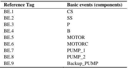
To illustrate the application of the proposed method, we use a benchmark case study of a simplified Cardiac Assist System (CAS) in [8]. The system consists of four modules: trigger, CPU unit, motor section, and pumps. The DFT of the CAS is shown in Fig.15. BEs of the DFT with their reference tags are shown in Table IV. As seen in the DFT, the trigger connected to the FDEP gate can become true due to the failure of either the crossbar switch (CS) or the system supervision (SS) or both. This trigger will cause both CPU units (P and B) to fail. The CPUs themselves are in warm spare configuration, where P is the primary unit and the B is the backup unit with a dormancy factor of 0.5. For the motor section of the system to fail, both MOTOR and MOTORC have to fail. The pump unit contains two cold spare gates and for the pump unit to fail the CSPGate_1 has to fail before CSPGate_2. CSPGate_1 and CSPGate_2 have PUMP_1 and PUMP_2 as their primary unit, respectively, and both CSP gates share a common spare (Backup_PUMP).
[image:11.576.50.532.343.701.2]
TABLEIV.THE CAS BASIC EVENTS (COMPONENTS) AND THEIR REFERENCE TAGS
Reference Tag Basic events (components)
BE.1 CS
BE.2 SS
BE.3 P
BE.4 B
BE.5 MOTOR
BE.6 MOTORC
BE.7 PUMP_1
BE.8 PUMP_2
BE.9 Backup_PUMP
We have considered that the failure rates of the BEs of the DFT are unknown. Following the process described in section III.B, the DFT in Fig. 15 is translated into a GSPN model and unknown failure rates of the BEs are collected according to the
process described in section III.C. The GSPN model of the DFT after incorporating the failure rates of the BEs (values for timed transitions) is shown in Fig. 16. For the data collection process for BEs, a heterogeneous group of experts was employed.
As it is evident from Table I, the experts’ weights are not same (see Table V). Four experts participated in this study to make the judgments. Two of them have a M.Sc. degree in systems engineering and had been working as system analysts for over 8 years. The third expert has a B.Sc. degree in manufacturing engineering and he had been working as a consultant and trainer for over four years. The last expert has a Ph.D. in industrial engineering and she had been working as an academic staff for over ten years. Job tenure and current activities of these experts are summarized in Table VI.
[image:12.576.54.262.82.193.2][image:12.576.130.448.270.715.2]
TABLEV.EXPERT WEIGHTING
Expert Professional position Job Experience Education Age Weighting score
Expert 1: Engineer (3) 6–9 (2) Master (4) (2) 11/49=0.22
Expert 2: Engineer (3) 6–9 (2) Master (4) (3) 12/49=0.24
Expert 3: Engineer (3) ≤ 5 (1) Bachelor (3) (3) 10/49=0.21 Expert 4: Senior academic (5) 10–19 (3) PhD (5) (3) 16/49=0.33
Total 49/49=1.00
TABLEVI.DETAILS OF THE EXPERTS
Board name Occupation Age Educational
Knowledge
Job tenure in Industry
Expert 1 (E1): System analyzer 36 Master of system engineering
He has been working as system analyzer for 9 years. He is currently the head of system analyzer in design department of a company.
Expert 2 (E2): System analyzer 42 Master of system engineering
She has been working as system analyzer for 8 years. She is currently vice head of system analyzer in design department of a company.
Expert 3 (E3): Consultant and trainer 43 Bachelor of manufacturing engineering
He has been working as a consultant and trainer since 2013. He is currently a member of safety department of automobile manufacturing.
Expert 4 (E4): Academic staff 41 PhD industrial engineering She has been working as an academic staff in industrial department for more than 10 years.
The experts’ decision on the BEs which have unknown failure rates is given in Table VII.
TABLEVII.EXPERTS’ DECISION ON THE UNKNOWN BES (COMPONENTS)
Reference Tag Experts
E1 E2 E3 E4
BE.1 VL L M VH
BE.2 M VL H VL
BE.3 H VL M H
BE.4 H M H M
BE.5 H M H VH
BE.6 VH H M L
BE.7 L VH H M
BE.8 M VH M VL
BE.9 M VH L H
The SAM technique was used to aggregate expert opinions for t=1000 hours. BE.1 is taken as an example and the details of aggregation are provided in Table VIII. To compute consensus coefficient using Equation (5), relaxation factor (β) is considered to be 0.5 to give the weight of the experts and their relative agreement an equal importance.
In addition, Equations (9) and (10) are applied to defuzzify the failure possibility of each BEs and also to transfer the corresponding fuzzy number to FP, respectively. The computation of BE.1 is done as an example and the results of other BEs are provided in Table IX.
Defuzzification 𝑜𝑓 BE. 1
=1
3(0.303 + 0.419 + 0.442 + 0.580
− 0.442 × 0.580 − 0.303 × 0.419 (0.442 + 0.580) − (0.303 + 0.419))
= 0. 437391
𝐾 = ( 1
0.437− 1)
1 3
⁄ × 2.301 =2.503
𝐹𝑃 = 1⁄102.503= 0.003145
From this FP value, using Equation (12) the failure rate is calculated as:
𝜆 =− ln(1 − 0.003145 ) 1000
=3.15E-06
[image:13.576.44.535.70.328.2] [image:13.576.58.257.388.508.2]TABLEVIII.AGGREGATION CALCULATIONS FOR THE BE.1 Expert 1 (0,0,0.1,0.2)
Expert 2 (0.1,0.25,0.25,0.4) Expert 3 (0.3,0.5,0.5,0.7) Expert 4 (0.8,0.9,1,1)
S(E1&E2) 0.825 𝑆(𝐴̃, 𝐵̃) = 1 −1
𝐽∑|𝑎𝑖− 𝑏𝑖|
𝐽
𝑖=1
S(E1&E3) 0.575 𝑆𝐸1,𝐸2= 1 − 1 4⁄ (0.1 + 0.25 + 0.15 + 0.2) = 0.825
S(E1&E4) 0.175 S(E2&E3) 0.75 S(E2&E4) 0.35 S(E3&E4) 0.6
AA(E1) 0.525 𝐴𝐴(𝐸𝑢) =
1
𝐽 − 1∑ 𝑆(𝑅̃𝑢, 𝑅̃𝑣)
𝐽
𝑢≠𝑣 𝑣=1
AA(E2) 0.642 1⁄(4 − 1)(0.825 + 0.575 + 0.175) = 0.525
AA(E3) 0.642 AA(E4) 0.375
RA(E1) 0.240 𝑅𝐴(𝐸𝑢) =
𝐴𝐴(𝐸𝑢)
∑ 𝐴𝐴(𝐸𝑢) 𝐽
𝑢=1
RA(E2) 0.294 0.525⁄(0.525 + 0.642 + 0.642 + 0.375)= 0.240
RA(E3) 0.294 RA(E4) 0.172
CC(E1) 0.230 𝐶𝐶(𝐸1) = 𝛽 ∙ 𝑊 (𝐸𝑢) + (1 − 𝛽) ⋅ 𝑅𝐴 (E1) =
CC(E2) 0.267 0.5 × 0.22 + 0.5 × 0.240 = 0.230 CC(E3) 0.252
CC(E4) 0.251
Aggregation for BE.1 𝑅̃AG = 𝐶𝐶(𝐸1) ⊗ 𝑅̃1⊕ 𝐶𝐶(𝐸2) ⊗ 𝑅̃2⊕ … ⊕ 𝐶𝐶(𝐸𝑚) ⊗ 𝑅̃𝑀
0.230⊗ (0,0,0.1,0.2) ⊕ 0.267⊗ (0.1,0.25,0.25,0.4) ⊕ 0.252⊗ (0.3,0.5,0.5,0.7) ⊕ 0.251⊗ (0.8,0.9,1,1) = (0.303,0.419,0.442,0.580)
TABLEIX.DEFUZZIFICATION OF NUMBERS AND CORRESPONDING FP OF EACH BES
Reference Tag Aggregated fuzzy set Defuzzification of BEs FP of BEs Failure rate
BE.1 (0.303,0.419,0.442,0.580) 0.437552 0.003149 3.15E-06
BE.2 (0.195,0.275,0.330,0.464) 0.318972 0.001089 1.09E-06
BE.3 (0.405,0.537,0.557,0.710) 0.553785 0.007225 7.25E-06
BE.4 (0.440,0.616,0.616,0.793) 0.616333 0.010847 1.09E-05
BE.5 (0.588,0.735,0.735,0.883) 0.735333 0.023080 2.34E-05
BE.6 (0.438,0.588,0.588,0.739) 0.588333 0.009062 9.10E-06
BE.7 (0.449,0.602,0.602,0.756) 0.602333 0.009917 9.97E-06
BE.8 (0.331,0.458,0.483,0.636) 0.478838 0.004296 4.31E-06
BE.9 (0.468,0.619,0.619,0.769) 0.618667 0.011009 1.11E-05
[image:14.576.110.490.72.427.2][image:14.576.80.509.76.717.2] [image:14.576.66.509.432.717.2]
TABLEX. CRITICALITY OF THE BASIC EVENTS OF THE DFT IN FIG.15
BEs Name BIM RANK
BE.1 0.625 1 BE.2 0.563 2 BE.3 0.251 5 BE.4 0.181 6 BE.5 0.261 4 BE.6 0.492 3 BE.7 0.040 7 BE.8 0.034 8 BE.9 0.022 9
V. CONCLUSION
Reliability analysis of complex and dynamic systems such as cyber physical systems is intricate. There are multiple stochastic and temporal dependencies that need to be taken into account and not all the existing stochastic formalisms are able to grasp these dependencies. Besides, the failure specification of some components, i.e., failure rate, is difficult to obtain. Frequently, the engineers have a qualitative knowledge about the possible failure behaviour, but with existing state-of-the-art methods this is not enough to quantify they system reliability.
In this context, this paper presents a novel uncertainty-aware dynamic reliability analysis approach. The approach enables the specification of failure data from expert judgement for components with unknown failure rates. Statistical, stochastic and temporal dependencies among events are treated in the analysis through Dynamic Fault Trees (DFT) and Generalised Stochastic Petri Nets (GSPN). There are other approaches that have addressed some of these issues in an isolated manner. However, to the best of the authors’ knowledge, not all issues have been covered in a single approach. Here this is achieved by combining DFT, GSPN, and fuzzy set theory.
The use of DFTs helped to model time-dependant failure behaviour, dependency among events, redundancy in the system model, and priorities among events. Fuzzy set theory and expert judgment enable us to collect uncertain failure data and also to explicitly highlight the areas of uncertainty in the data. GSPN was used to take into account the statistical and stochastic dependencies among events, which helped to avoid inaccurate reliability estimation of the system by performing analysis under realistic assumptions.
The effectiveness of the approach was demonstrated via application to a benchmark case study. The result obtained is believed to be improved and more useful than results derived with more traditional approaches due to the combined capabilities of the method.
The use of expert judgement in estimating failure probabilities of BEs is not expected to be faultless, but can contribute to usefully quantifying what was previously unquantifiable. Note that the current method only obtained an exponentially distributed failure rate, however, to utilise the full potential of GSPN, it would be worthwhile to explore
methods to obtain the failure rate function for other distributions. The criticality analysis allows analysts to identify weak areas of the system early and to focus redesign efforts correspondingly. The extent of scalability of this approach for the analysis of large-scale systems is not yet determined. It could be the case that GSPNs grow to sizes that make computations very demanding. However, if issues arise then modularisation techniques such as [68]-[71] may help to improve scalability of the analysis.
REFERENCES
[1] J. B. Dugan, S. J. Bavuso, and M. A. Boyd, “Dynamic fault-tree models for fault-tolerant computer systems,” IEEE Trans. Reliab., vol. 41, no. 3, pp. 363–377, 1992.
[2] G. K. Palshikar, “Temporal fault trees,” Inf. Softw. Technol., vol. 44, no. 3, pp. 137–150, 2002.
[3] M. Walker, “Pandora: A Logic for the Qualitative Analysis of Temporal Fault Trees,” PhD Thesis, University of Hull, 2009. [4] G. Merle, J. Roussel, J. Lesage, and A. Bobbio, “Probabilistic Algebraic Analysis of Fault Trees With Priority Dynamic Gates and Repeated Events,” IEEE Trans. Reliab., vol. 59, no. 1, pp. 250–261, 2010.
[5] G. Merle, J.-M. Roussel, and J.-J. Lesage, “Algebraic
determination of the structure function of Dynamic Fault Trees,” Reliab. Eng. Syst. Saf., vol. 96, no. 2, pp. 267–277, Feb. 2011. [6] H. Boudali, P. Crouzen, and M. Stoelinga, “A Rigorous,
Compositional, and Extensible Framework for Dynamic Fault Tree Analysis,” IEEE Trans. Dependable Secur. Comput., vol. 7, no. 2, pp. 128–143, Apr. 2010.
[7] J. B. Dugan, S. J. Bavuso, and M. A. Boyd, “Fault trees and Markov models for reliability analysis of fault-tolerant digital systems,” Reliab. Eng. Syst. Saf., vol. 39, no. 3, pp. 291–307, 1993.
[8] H. Boudali and J. B. Dugan, “A discrete-time Bayesian network reliability modeling and analysis framework,” Reliab. Eng. Syst. Saf., vol. 87, no. 3, pp. 337–349, 2005.
[9] H. Boudali and J. B. Dugan, “A Continuous-Time Bayesian Network Reliability Modeling, and Analysis Framework,” IEEE Trans. Reliab., vol. 55, no. 1, pp. 86–97, 2006.
[10] S. Montani, L. Portinale, A. Bobbio, and D. Codetta-Raiteri, “Radyban: A tool for reliability analysis of dynamic fault trees through conversion into dynamic Bayesian networks,” Reliab. Eng. Syst. Saf., vol. 93, no. 7, pp. 922–932, Jul. 2008. [11] D. Marquez, M. Neil, and N. Fenton, “Improved reliability
modeling using Bayesian networks and dynamic discretization,” Reliab. Eng. Syst. Saf., vol. 95, no. 4, pp. 412–425, Apr. 2010. [12] M. A. Marsan and G. Chiola, “On Petri nets with deterministic and exponentially distributed firing times,” Adv. Petri Nets, vol. 266, pp. 132–145, Jun. 1987.
[13] D. Codetta-Raiteri and L. Portinale, “Generalized Continuous Time Bayesian Networks as a modelling and analysis formalism for dependable systems,” Reliab. Eng. Syst. Saf., vol. 167, pp. 639–651, 2017.
[14] H. Tanaka, L. T. Fan, F. S. Lai, and K. Toguchi, “Fault-Tree Analysis by Fuzzy Probability,” IEEE Trans. Reliab., vol. R-32, no. 5, pp. 453–457, Dec. 1983.
[15] S. Kabir, “An overview of Fault Tree Analysis and its application in model based dependability analysis,” Expert Syst. Appl., vol. 77, pp. 114–135, 2017.
[16] Y.-F. Li, J. Mi, Y. U. Liu, Y.-J. Yang, and H.-Z. Huang, “Dynamic fault tree analysis based on continuous-time Bayesian networks under fuzzy numbers,” Proc. Inst. Mech. Eng. Part O J. Risk Reliab., vol. 229, no. 6, pp. 530–541, 2015.
[image:15.576.95.219.76.185.2][18] Y. F. Li, H. Z. Huang, Y. Liu, N. Xiao, and H. Li, “A new fault tree analysis method : fuzzy dynamic fault tree analysis,” Eksploat. i Niezawodn. Reliab., vol. 14, no. 3, pp. 208–214, 2012.
[19] Y. Ren, D. Fan, X. Ma, Z. Wang, Q. Feng, and D. Yang, “A GO-FLOW and Dynamic Bayesian Network Combination Approach for Reliability Evaluation With Uncertainty: A Case Study on a Nuclear Power Plant,” IEEE Access, vol. 6, pp. 7177–7189, 2018.
[20] A. Toppila and A. Salo, “A Computational Framework for Prioritization of Events in Fault Tree Analysis Under Interval-Valued Probabilities,” IEEE Trans. Reliab., vol. 62, no. 3, pp. 583–595, Sep. 2013.
[21] A. Rajan, M. P.-L. Ooi, Ye Chow Kuang, and S. N. Demidenko, “Analytical Standard Uncertainty Evaluation Using Mellin Transform,” IEEE Access, vol. 3, pp. 209–222, 2015. [22] A. P. Ulmeanu, “Analytical Method to Determine Uncertainty
Propagation in Fault Trees by Means of Binary Decision Diagrams,” IEEE Trans. Reliab., vol. 61, no. 1, pp. 84–94, Mar. 2012.
[23] X. Song, Z. Zhai, P. Zhu, and J. Han, “A Stochastic Computational Approach for the Analysis of Fuzzy Systems,” IEEE Access, vol. 5, pp. 13465–13477, 2017.
[24] H. A. Watson, “Launch control safety study,” Murray Hill, New Jersey, 1961.
[25] T. Murata, “Petri Nets : Properties , Analysis and Applications,” Proc. IEEE, vol. 77, no. 4, pp. 541–580, 1989.
[26] M. K. Molloy, “Performance analysis using stochastic Petri nets,” IEEE Trans. Comput., vol. c-31, no. 9, pp. 913–917, 1982. [27] B. Beyaert, G. Florin, P. Lonc, and S. Natkin, “Evaluation of
computer systems dependability using stochastic Petri nets,” in Digest of the 11th Annual Symposium on Fault-Tolerant Computing, 1981, pp. 79–81.
[28] N. G. Leveson and J. L. Stolzy, “Safety Analysis Using Petr Nets,” IEEE Trans. Softw. Eng., vol. 13, no. 3, pp. 386–397, 1987.
[29] G. S. Hura and J. W. Atwood, “The Use Of Petri Nets To Analyze Coherent Fault Trees,” IEEE Trans. Reliab., vol. 37, no. 5, pp. 469–474, 1988.
[30] A. Bobbio, G. Franceschinis, R. Gaeta, and L. Portinale, “Exploiting Petri Nets to Support Fault Tree Based Dependability Analysis,” in 8th International Workshops on Petri Nets and Performance Models, 1999, pp. 146–155. [31] D. Codetta-Raiteri, “The Conversion of Dynamic Fault Trees to
Stochastic Petri Nets, as a case of Graph Transformation,” Electron. Notes Theor. Comput. Sci., vol. 127, no. 2, pp. 45–60, Mar. 2005.
[32] S. Kabir, M. Walker, and Y. Papadopoulos, “Quantitative evaluation of Pandora Temporal Fault Trees via Petri Nets,” IFAC-PapersOnLine, vol. 48, no. 21, pp. 458–463, 2015. [33] S. Kabir, M. Walker, and Y. Papadopoulos, “Dynamic system
safety analysis in HiP-HOPS with Petri Nets and Bayesian Networks,” Saf. Sci., vol. 105, pp. 55–70, Jun. 2018.
[34] L. Zadeh, “Fuzzy Sets,” Inf. Control, vol. 8, no. 3, pp. 338–353, 1965.
[35] Y. Hong, H. J. Pasman, S. Sachdeva, A. S. Markowski, and M. S. Mannan, “A fuzzy logic and probabilistic hybrid approach to quantify the uncertainty in layer of protection analysis,” J. Loss Prev. Process Ind., vol. 43, pp. 10–17, 2016.
[36]
T. J. Ross, Fuzzy Logic with Engineering Applications. 2009. [37] K. T. Atanassov, “Intuitionistic fuzzy sets,” Fuzzy Sets Syst., vol.
20, no. 1, pp. 87–96, 1986.
[38] S.-J. Chen and C.-L. Hwang, “Fuzzy Sets and Their Operations,” in Fuzzy Multiple Attribute Decision Making, 1992, pp. 42–100. [39] K. T. Atanassov, “On the Concept of Intuitionistic Fuzzy Sets,”
in On Intuitionistic Fuzzy Sets Theory, 2012, pp. 1–16. [40] W. E. Vesely, M. Stamatelatos, J. Dugan, J. Fragola, J.
Minarick, and J. Railsback, “Fault tree handbook with aerospace applications.” NASA Office of Safety and Mission Assurance, Washington DC,USA, 2002.
[41] S. Banerjee, Industrial hazards and plant safety. Taylor & Francis, 2003.
[42] B. M. Ayyub, Risk Analysis in Engineering and Economics, Second Edition. 2014.
[43] M. Modarres, M. Kaminskly, and V. Krivtsov, Reliability Engineering and Risk Analysis. 1999.
[44] M. Malhotra and K. S. Trivedi, “Dependability Modeling Using Petri-Nets,” IEEE Trans. Reliab., vol. 44, no. 3, pp. 428–440, 1995.
[45] M. Rausand, Reliability of safety-critical systems. 2014. [46] OREDA, Offshore Reliability Data Handbook, 4. ed.
Trondheim, 2002.
[47] C. Preyssl, “Safety risk assessment and management-the ESA approach,” Reliab. Eng. Syst. Saf., vol. 49, no. 3, pp. 303–309, 1995.
[48] M. Yazdi, “Hybrid Probabilistic Risk Assessment Using Fuzzy FTA and Fuzzy AHP in a Process Industry,” J. Fail. Anal. Prev., vol. 17, no. 4, pp. 756–764, 2017.
[49] S. Greco, J. Figueira, and M. Ehrgott, Multiple criteria decision analysis. Springer’s International series, 2005.
[50]
M. Yazdi and E. Zarei, “Uncertainty Handling in the Safety Risk Analysis: An Integrated Approach Based on Fuzzy Fault Tree Analysis,” J. Fail. Anal. Prev., vol.18, no. 2, pp. 392-404, 2018. [51]
F. Aqlan and E. Mustafa Ali, “Integrating lean principles and
fuzzy bow-tie analysis for risk assessment in chemical industry,” J. Loss Prev. Process Ind., vol. 29, no. 1, pp. 39–48, 2014. [52] Y. Liu, Z. P. Fan, Y. Yuan, and H. Li, “A FTA-based method for
risk decision-making in emergency response,” Comput. Oper. Res., vol. 42, pp. 49–57, 2014.
[53] M. Yazdi, F. Nikfar, and M. Nasrabadi, “Failure probability analysis by employing fuzzy fault tree analysis,” Int. J. Syst. Assur. Eng. Manag., pp. 1–17, 2017.
[54] M. Yazdi, “The Application of Bow-Tie Method in Hydrogen Sulfide Risk Management Using Layer of Protection Analysis (LOPA),” J. Fail. Anal. Prev., vol. 17, no. 2, pp. 291–303, 2017. [55] S. M. Lavasani, N. Ramzali, F. Sabzalipour, and E. Akyuz,
“Utilisation of Fuzzy Fault Tree Analysis (FFTA) for quantified risk analysis of leakage in abandoned oil and natural-gas wells,” Ocean Eng., vol. 108, pp. 729–737, 2015.
[56] N. Ramzali, M. R. M. Lavasani, and J. Ghodousi, “Safety barriers analysis of offshore drilling system by employing Fuzzy event tree analysis,” Saf. Sci., vol. 78, pp. 49–59, 2015. [57] S. M. Lavasani, J. Wang, Z. Yang, and J. Finlay, “Application of
fuzzy fault tree analysis on oil and gas offshore pipelines,” Int. J. Mar. Sci. Eng., vol. 1, no. 1, pp. 29–42, 2011.
[58] S. M. Lavasani, A. Zendegani, and M. Celik, “An extension to Fuzzy Fault Tree Analysis (FFTA) application in petrochemical process industry,” Process Saf. Environ. Prot., vol. 93, pp. 75– 88, Jan. 2015.
[59] M. Yazdi and S. Kabir, “A Fuzzy Bayesian Network approach for Risk Analysis in Process Industries,” Process Saf. Environ. Prot., vol. 111, pp. 507–519, Aug. 2017.
[60] J. S. Nicolis and I. Tsuda, “Chaotic dynamics of information processing: The ‘magic number seven plus-minus two’ revisited,” Bull. Math. Biol., vol. 47, no. 3, pp. 343–365, 1985. [61] G. Miller, “The magical number seven, plus or minus two: some
limits on our capacity for processing information.,” Psychol. Rev., vol. 101, no. 2, pp. 343–352, 1956.
[62] H.-M. Hsu and C.-T. Chen, “Aggregation of fuzzy opinions under group decision making,” Fuzzy Sets Syst., vol. 79, no. 3, pp. 279–285, 1996.
[63] R. Zhao and R. Govind, “Defuzzification of fuzzy intervals,” Fuzzy Sets Syst., vol. 43, no. 1, pp. 45–55, 1991.
[64] M. Sugeno, H. T. Nguyen, and N. R. Prasad, Fuzzy modeling and control : selected works of M. Sugeno. CRC Press, 1999. [65] T. Onisawa, “A representation of human reliability using fuzzy
concepts,” Inf. Sci. (Ny)., vol. 45, no. 2, pp. 153–173, 1988. [66] T. Onisawa, “An application of fuzzy concepts to modelling of
reliability analysis,” Fuzzy Sets Syst., vol. 37, no. 3, pp. 267– 286, 1990.
[68] R. Gulati and J. B. Dugan, “A Modular Approach for Analyzing Static and Dynamic Fault Trees,” in Proceedings of the Annual Reliability and Maintainability Symposium, 1997, pp. 57–63. [69] R. Manian, J. B. Dugan, D. Coppit, and K. J. Sullivan,
“Combining Various Solution Techniques for Dynamic Fault Tree Analysis of Computer Systems,” in Proceedings of Third IEEE International High-Assurance Systems Engineering Symposium, 1998, pp. 21–28.
[70] C.-Y. Huang and Y.-R. Chang, “An improved decomposition scheme for assessing the reliability of embedded systems by using dynamic fault trees,” Reliab. Eng. Syst. Saf., vol. 92, no. 10, pp. 1403–1412, 2007.
[71] F. Chiacchio, M. Cacioppo, D. D’urso, G. Manno, N. Trapani, and L. Compagno, “A Weibull-based compositional approach for hierarchical dynamic fault trees,” Reliab. Eng. Syst. Saf., vol. 109, pp. 45–52, 2013.
Sohag Kabir is a research associate in the Dependable Intelligent Systems (DEIS) Research Group at the University of Hull. He received his PhD in Computer Science and MSc degree in Embedded Systems from the University of Hull, UK in 2016 and 2012, respectively. He has worked in EU projects on safety including MAENAD and DEIS. His research interests include model-based safety assessment, probabilistic risk and safety analysis, dynamic safety and reliability analysis, and stochastic modelling and analysis.
Mohammad Yazdi received the M.Sc degree in Industrial Engineering from Eastern Mediterranean University, Famagusta, Cyprus in 2017, and the B.Sc degree in process safety engineering from Petroleum University of Technology, Abadan, Iran in 2012.
He is currently pursuing the Ph.D. degree with the Centre for Marine Technology and Ocean Engineering (CENTEC), University of Lisbon. His research mainly focuses on risk assessment based on uncertainty handling. Before undertaking the academic career, he served as a safety expert and auditor in oil and gas industry from 2012 to 2016.
Jose Ignacio Aizpurua(M’17) is a Research Associate within the Institute for Energy and Environment at the University of Strathclyde, Scotland, UK. He received his Eng., M.Sc., and Ph.D. degrees from Mondragon University (Spain) in 2010, 2012, and 2015 respectively. He was a visiting researcher in the Dependable Systems Research group at the University of Hull (UK) in 2014. His research interests include prognostics and health management, reliability, availability, maintenance and safety (RAMS) analysis and systems engineering for power engineering applications.
![FIGURE 4. Diagrams for a classical set (Boolean) and a fuzzy set [35].](https://thumb-us.123doks.com/thumbv2/123dok_us/1388846.92030/4.576.43.274.522.611/figure-diagrams-classical-set-boolean-fuzzy-set.webp)

![TABLE II. QUALITATIVE TERMS AND THEIR CORRESPONDING FUZZY NUMBERS [38]](https://thumb-us.123doks.com/thumbv2/123dok_us/1388846.92030/9.576.39.280.65.177/table-ii-qualitative-terms-corresponding-fuzzy-numbers.webp)
![FIGURE 15. The CAS dynamic fault tree (modified after [8]).](https://thumb-us.123doks.com/thumbv2/123dok_us/1388846.92030/11.576.50.532.343.701/figure-cas-dynamic-fault-tree-modified.webp)