Abstract—Although Extreme Learning Machines (ELM)
have been successfully applied for the classification of hyperspectral images (HSIs), they still suffer from three main drawbacks. These include: 1) Ineffective feature extraction in HSIs due to a single hidden layer neuron network used; 2) ill-posed problems caused by the random input weights and biases; and 3) lack of spatial information for HSIs classification. To tackle the first problem, we construct a multilayer ELM for effective feature extraction from HSIs. The sparse representation is adopted with the multilayer ELM to tackle the ill-posed problem of ELM, which can be solved by the alternative direction method of multipliers (ADMM). This has resulted in the proposed multilayer sparse ELM (MSELM) model. Considering that the neighboring pixels are more likely from the same class, a local block extension is introduced for MSELM to extract the local spatial information, leading to the local block MSELM (LBMSLM). The loopy belief propagation (LBP) is also applied to the proposed MSELM and LBMSELM approaches to further utilize the rich spectral and spatial information for improving the classification. Experimental results show that the proposed methods have outperformed the ELM and other state-of-the-art approaches.
Index Terms—Extreme learning machine (ELM); hyperspectral images (HSI); local block multilayer sparse ELM (LBMSELM); loopy belief propagation (LBP); alternative direction method of multipliers (ADMM).
I. INTRODUCTION
n the last 1-2 decades, hyperspectral images (HSIs) have been widely and successfully applied in many application fields, such as crop analysis, geological research, environment mapping and the geology [1-4]. A pixel in HSIs is a
This work is supported in part by the National Nature Science Foundation of China (no. 61471132), the Training program for outstanding young teachers of Guangdong Province (no. YQ2015057) the High-Level University Construction Funds of Guangdong University of Technology (no. 1109/220410011) and the Innovation Team Project of Guangdong Education Department (no. 2017KCXTD011). Corresponding author: Dr. Zhijing Yang.
F. Cao, Z. Yang, W. Chen and G. Han are with School of Information Engineering, Guangdong University of Technology, Guangzhou, China. ([email protected], [email protected], [email protected],
F. Cao and J. Ren are with Department of Electronic and Electrical Engineering, University of Strathclyde, Glasgow, UK. ([email protected],[email protected]).
Y. Shen is the Department of Guangzhou Urban Planning Technology Development Services, Guangzhou, China. ([email protected])
high-dimensional vector which contains the spectral responses from various spectral bands. Depending on the specific spectral range, the rich spectral information in HSIs allows to classify and identify from each pixel with certain physical and chemical parameters, such as temperature, moisture and chemical components [5]. Although relatively good results of classification have been reported, mainly using supervised learning, accurate classification of HSI remains a challenging problem due to the Hughes phenomenon [6], which is caused by the ratio of the large number of spectral bands and limited samples of training pixels. Besides, the materials from the same category may have different spectral features whilst different classes of samples may share similar spectral characteristic due to noise of the sensors and environments [7].
To tackle these problems, a number of state-of-the-art algorithms have been proposed, such as the support vector machine [8] (SVM), the multi-kernel classification [9] (MK), the sparse multinomial logistic regression [10-11] and the extreme learning machine [12-13] (ELM). Besides, a number of methods have also been proposed for feature extraction, such as principal component analysis (PCA) and its variations [14-16], segmented auto-encoder [17] and singular spectrum analysis (SSA) [18-20]. Among these algorithms, the ELM has attracted much attention in terms of its good performance. ELM has been proven a promise algorithm in many applications due to its fast implementation, straightforward solution and strong generalization capability [13, 21-23]. In [24-25], a theoretical assessment has shown the feasible performance of ELM. In [26], a regularized ELM has been proposed for regression with missing data. In [27], the ELM auto-encoder has been proposed for dimension reduction and feature extraction. ELM has also been applied for HSIs classification [28-32], for example, in [28-29], local binary patterns were used for feature extraction, followed by ELM for classification. In [30-31], ELM was employed for classification with features extracted using extended morphological profiles and bilateral filtering, respectively. In [32], an optimized extreme learning machine (OELM) was proposed for urban land cover classification in HSIs. Although ELM has achieved good performance in classification of HSI to some extent, three major deficiencies of ELM can be depicted as follows: i) Ineffective feature extraction due to its architecture of a single hidden layer feedforward neuron network; ii) the ill-posed problem of ELM caused by the random input weight and bias of ELM; and iii) lack of capability of extracting the rich spatial
Local Block Multilayer Sparse Extreme Learning
Machine for Effective Feature Extraction and
Classification of Hyperspectral Images
Faxian Cao,
Student Member, IEEE,
Zhijing Yang,
Member, IEEE,
Jinchang Ren,
Senior
Member, IEEE,Weizhao Chen,
Guojun Han,
Senior
Member, IEEE, Yuzhen Shen
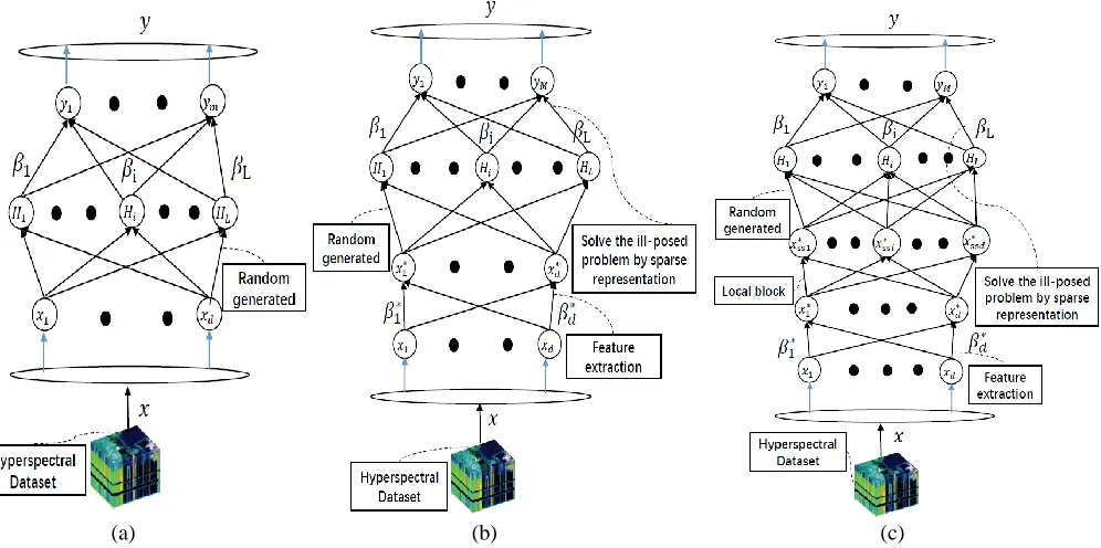
information of HSIs. To tackle these three problems, we propose a multilayer sparse ELM (MSELM) and a further extended local block MSELM (LBMSELM) for effective feature extraction and classification of HSIs. Fig. 1 shows the workflows of the original ELM, and the proposed MSELM and LBMSELM algorithms for comparison.
First, feature extraction is crucial for effective classification of HSIs. To this end, we aim to design a multilayer ELM to extract the efficient feature in order to realize the high classification accuracies. For the ill-posed problem caused by the random weights and bias, we impose the sparse representation to ELM. We construct the optimization function to realize the multilayer sparse ELM (MSELM) which can be solved by the alternative direction method of multiplier (ADMM) [33]. Details will be discussed in Section III-A.
Second, due to the homogenous regions in HSIs where the neighborhood pixels within the regions consist of the same class materials or share similar spectral characteristics [34], neighboring pixels in spatial domain more likely belong to the same class [31]. In view of this, we further introduce the spatial information to the proposed MSELM to reduce the classification error. A local block area for each training pixel of HSIs is constructed and imposed to the optimization problem of the proposed MSELM in order to incorporate the spectral and spatial information in HSIs, namely local block MSELM (LBMSELM). More details can be found in Section III-B.
The main contributions of this paper can be summarized as follows. First, we design a new ELM-based algorithm, called MSELM, for efficient feature extraction of HSIs and solving the ill-posed problem of ELM caused by random weights and bias. Second, we develop the proposed MSELM in order to reveal the local neighboring information in HSIs, namely LBMSELM. Comprehensive experiments have fully demonstrated the efficacy of the proposed methodologies.
The rest of this paper is organized as follows. Section II describes the background of ELM. In Section III, the proposed frameworks are presented. The experiment results and analysis are given in Section IV. Section V concludes this paper with some remarks and suggestions.
II. EXTREME LEARNING MACHINE (ELM)
ELM is a generalized single layer feedforward neural network, where the weight vector and bias are randomly generated at the beginning of the learning process [32, 35]. Given N training samples 𝑋 ≡ (𝑥1; 𝑥2; … ; 𝑥𝑁) ∈ 𝑅𝑁×𝑑 of a HSI, where d denotes the number of spectral bands, the corresponding labels of the given N training samples are denoted by 𝑌 = (𝑦1; 𝑦2; … ; 𝑦𝑁) ∈ 𝑅𝑁×𝑀, where M is the number of classes in the HSI that needs to be classified. If the i-th training sample belongs to the m-th class, we have
𝑦𝑖,𝑗= { 0, 𝑜𝑡ℎ𝑒𝑟𝑤𝑖𝑠𝑒.1, 𝑗 = 𝑚, (1) The ELM model with L hidden neurons and the activation function 𝐻(𝑥) [29] can be expressed as follows:
∑𝐿𝑗=1𝛽𝑗𝐻(𝑤𝑗𝑇∗ 𝑥𝑖+ 𝑏𝑗) = 𝑦𝑖, i=1,2,…,N (2) where 𝑤𝑗 and 𝑏𝑗 represent the weight vector and bias between input layer and hidden layer of ELM, respectively, and 𝛽𝑗 is the weight vector from the hidden layer to the output layer. 𝐻(𝑤𝑗𝑥𝑖+ 𝑏𝑗) is the output of the j-th hidden neuron corresponding to the input sample 𝑥𝑖.
The solution of 𝛽 in Eq. (2) can be directly obtained by:
𝛽 = 𝐻†𝑌 (3)
[image:2.612.59.557.55.303.2]where 𝛽 = [𝛽1, 𝛽2, … , 𝛽𝑀] ∈ 𝑅𝐿×𝑀 , and 𝐻† is the Moore-Penrose generalized inverse of matrix 𝐻 [36]. That is
𝐻†= 𝐻𝑇(𝐻𝐻𝑇)−1 or 𝐻†= (𝐻𝑇𝐻)−1𝐻𝑇 and
𝐻 = [ℎ(𝑤1, 𝑏⋮1, 𝑥1) ⋯ ℎ(𝑤⋱ 1, 𝑏⋮1, 𝑥𝑁) ℎ(𝑤𝐿, 𝑏𝐿, 𝑥1) ⋯ ℎ(𝑤𝐿, 𝑏𝐿, 𝑥𝑁)
] (4)
Although ELM has many merits, it still has three main drawbacks: 1) As a single hidden layer feedforward neural network, ELM can’t effectively extract the features for classification of HSIs; 2) The random weights and bias of ELM will cause the ill-posed problem; and 3) The ELM can’t extract the useful spatial information for HSI classification hence the performance is constrained. To tackle these drawbacks, we propose the local block multilayer sparse extreme learning machine (LBMSELM) as detailed in the next section.
III. THE PROPOSED FRAMEWORK
A. Multilayer Sparse Extreme Learning Machine (MSELM)
Given N training samples 𝑋 ≡ (𝑥1; 𝑥2; … ; 𝑥𝑁 ) ∈ 𝑅𝑁×𝑑 and the corresponding labels 𝑌 = (𝑦1; 𝑦2; … ; 𝑦𝑁) ∈ 𝑅𝑁×𝑀, the feature extraction problem can be formulated as:
𝑋 = 𝑋∗+ 𝜓 (5) where 𝑋∗= (𝑥1∗, 𝑥2∗, … , 𝑥𝑁∗) ∈ 𝑅𝑁×𝑑 is the features extracted from X, and ψ is the redundancy feature of X. Then we can rewrite Eq. (5) as follows:
𝑋 = 𝑋𝛽∗+ 𝜓 (6) where 𝛽∗= (𝛽1∗, 𝛽2∗, … , 𝛽𝑑∗) ∈ 𝑅𝑑×𝑑. From Eq. (6), we can see that we aim to find a term β∗to extract features from X, i.e.
X∗= Xβ∗
. Based on ELM, an optimization problem can be constructed to minimize the redundancy feature and classification error for improved classification as defined by:
𝑚𝑖𝑛
𝛽,𝛽∗ ∥ 𝑋 − 𝑋𝛽
∗∥ 𝐹
2+∥ 𝑌 − 𝐻∗𝑇𝛽 ∥ 𝐹
2 (7)
𝐻∗= [𝐻∗(𝑥
1∗), 𝐻∗(𝑥2∗), … , 𝐻∗(𝑥𝑁∗)] =
[ℎ
∗(𝑤
1, 𝑏1, 𝑥1∗) ⋯ ℎ∗(𝑤1, 𝑏1, 𝑥𝑁∗)
⋮ ⋱ ⋮
ℎ∗(𝑤
𝐿, 𝑏𝐿, 𝑥1∗) ⋯ ℎ∗(𝑤𝐿, 𝑏𝐿, 𝑥𝑁∗)
] (8)
where T is the matrix transpose; 𝛽 = (𝛽1, 𝛽2, … , 𝛽𝑀) ∈ 𝑅𝐿×𝑀. Our aim is to construct a multilayer sparse extreme learning machine (MSELM) to extract effective features and solve the ill-posed problem of ELM that may lead to relatively low classification accuracy. According to Bartlett’s generalization theory [37], the smaller weight will result in less training error of the training model. To this end, the optimization model of MSELM is rewritten as:
𝑚𝑖𝑛
(𝛽,𝛽∗)
1
2∥ 𝛽∗ ∥𝐹2+ 𝐶 2⁄ ∥ 𝜓𝑖∥22+
1
2∥ 𝑌 − 𝐻∗𝑇𝛽 ∥𝐹2+ 𝜆 ∥ 𝛽 ∥1
𝑠. 𝑡. 𝑥𝑖− 𝑥𝑖𝛽∗= 𝜓𝑖; i=1,2,..N (9) where 𝜓 = (𝜓1; 𝜓2; … ; 𝜓𝑁) ∈ 𝑅𝑁×𝑑. As seen in Eq. (9), the sparse representation is imposed to ELM, and the variable
splitting principle [38] is adopted which consists a procedure to create new variables. The model in Eq. (9) is equal to
𝑚𝑖𝑛
(𝛽,𝛽∗,𝑣)
1
2∥ 𝛽∗ ∥𝐹2+ 𝐶 2⁄ ∥ 𝜓𝑖∥22+
1
2∥ 𝑌 − 𝐻∗𝑇𝛽 ∥𝐹2+ 𝜆 ∥ 𝑣 ∥1
𝑠. 𝑡. 𝑥𝑖∗− 𝑥𝑖𝛽∗= 𝜓𝑖; 𝑣= 𝛽; i=1,2,..N (10) Applying the augmented Lagrangian [39] to Eq. (10), the above MSELM model can be solved by ADMM algorithms [33] as follows.
𝛽∗= 𝑎𝑟𝑔 min 𝛽∗ {
1 2∥ 𝛽
∗ ∥ 𝐹 2
+ 𝐶 2⁄ ∑𝑁𝑖=1∥ 𝜓𝑖∥22+
∑𝑖=1𝑁 ∑𝑑𝑚=1𝛾𝑖,𝑚(𝑥𝑖− 𝑥𝑖𝛽∗− 𝜓𝑖)} (11)
𝛽𝑡+1= 𝑎𝑟𝑔 min 𝛽 {
1
2∥ 𝑌 − 𝐻 ∗𝑇𝛽 ∥
𝐹 2+𝜆∗
2 ∥ 𝛽 − 𝑣 𝑡− 𝑑𝑡∥
𝐹 2} (12)
𝑣𝑡+1= 𝑎𝑟𝑔 min
𝑣 { 𝜆 ∥ 𝑣 ∥1+ 𝜆∗
2 ∥ 𝛽
𝑡+1− 𝑣 − 𝑑𝑡∥ 𝐹
2} (13)
𝑑𝑡+1= 𝑑𝑡− (𝛽𝑡+1− 𝑣𝑡+1) (14) where 𝛾 = [𝛾1; 𝛾2; … ; 𝛾𝑁] ∈ 𝑅𝑁×𝑑 is the Lagrange multiplies.
𝛽∗ can be obtained by the Karush-Kuhn-Tucker (KKT) theory [40], that is to say:
𝛽∗= 𝑋𝑇(𝐼2
𝐶+ 𝑋𝑋
𝑇)−1𝑋 (15)
𝛽𝑡+1 can be solved by the first-order derivation:
𝛽𝑡+1= (𝐻∗𝐻∗𝑇+ 𝜆∗𝐼)−1(𝐻∗𝑌 + 𝜆∗(𝑣𝑡+ 𝑑𝑡)) (16) The 𝑣𝑡+1 can be solved by a simple soft-threshold [38] as:
𝑣𝑡+1= 𝑠𝑜𝑓𝑡(𝛽𝑡+1− 𝑑𝑡,𝜆𝜆∗) (17) where 𝑡 is the index of iterations; 𝜆 and 𝜆∗ are all positive values; 𝐼 is an identity matrix, whose dimension is corresponding to the dimension of H∗H∗𝑇. We set 𝜆∗= 10𝜆 for easy implementation and parameter tuning.
Let 𝑋̂ = (𝑥̂1, 𝑥̂2, … , 𝑥̂𝑛) ∈ 𝑅𝑛×𝑑 be the two-dimensional (2-D) representation of n testing samples in a given HSI, the test process of the proposed MSELM can be achieved by:
𝑓(𝑥̂𝑖) = 𝐻∗(𝑥̂𝑖∗)𝛽 = 𝐻∗(𝑥̂𝑖∗)𝑇(𝐻∗𝐻∗𝑇+ 𝜆∗𝐼) −1
(𝐻∗𝑌 + 𝜆∗(𝑣 + 𝑑)) i=1,2,..,n, (18) where 𝐻∗(𝑥̂𝑖∗) = [ℎ∗(𝑤1, 𝑏1, 𝑥̂𝑖𝛽∗), … , ℎ∗(𝑤L, 𝑏L, 𝑥̂𝑖𝛽∗)]𝑇 and
𝑥̂𝑖∗= 𝑥̂𝑖𝛽∗ .The pseudocodes for MSELM are given in Algorithm 1.
B. Local Block MSELM (LBMSELM)
For the 2-D representation of an HSI 𝑋̂ = (𝑥̂1, 𝑥̂2, … , 𝑥̂𝑛) ∈
𝑥1∗; 𝑥2∗; … ; 𝑥𝑁∗; 𝑥11∗ ; 𝑥21∗ ; … ; 𝑥𝑁1∗ ; … ; 𝑥1𝑝∗ ; 𝑥2𝑝∗ ; … ; 𝑥𝑁𝑝∗ ) ∈
𝑅(𝑝+1)𝑁×𝑑, where p denotes the number of the pixels used in the neighborhoods of each training pixel. As such, the training model of LBMSELM can be defined by:
𝛽𝑆𝑆𝑡+1= (𝐻𝑆𝑆∗𝐻𝑆𝑆∗ 𝑇+ 𝜆∗𝐼) −1
(𝐻𝑆𝑆∗𝑌∗+ 𝜆∗(𝑣𝑆𝑆𝑡 + 𝑑𝑆𝑆𝑡 )) (20)
𝑣𝑆𝑆𝑡+1= soft(𝛽𝑆𝑆𝑡+1− 𝑑𝑆𝑆𝑡 ,𝜆𝜆∗) (21)
𝑑𝑆𝑆𝑡+1= 𝑑𝑆𝑆𝑡 − (𝛽𝑆𝑆𝑡+1− 𝑣𝑆𝑆𝑡+1) (22) where 𝐼 is an identity matrix and its dimension depends on the dimension of 𝐻𝑆𝑆∗ 𝐻𝑆𝑆∗ 𝑇, 𝑌∗= (𝑌, 𝑌, . . , 𝑌) ∈ 𝑅(𝑝+1)𝑁×𝑀, and
𝐻𝑆𝑆∗ ∈ 𝑅𝐿×(𝑝+1)𝑁 is given by
𝐻𝑆𝑆∗ = [
ℎ∗(𝑤
1, 𝑏1, 𝑥1∗) ⋯ ℎ∗(𝑤1, 𝑏1, 𝑥𝑁𝑝∗ )
⋮ ⋱ ⋮
ℎ∗(𝑤
L, 𝑏L, 𝑥1∗) ⋯ ℎ∗(𝑤𝐿, 𝑏𝐿, 𝑥𝑁𝑝∗ )
] (23)
The testing process of the proposed LBMSELM is given by:
𝑓(𝑥̂𝑖) = 𝐻𝑆𝑆∗ (𝑥̂𝑖∗)𝑇𝛽𝑆𝑆= 𝐻𝑆𝑆∗ (𝑥̂𝑖∗)𝑇(𝐻𝑆𝑆∗𝐻𝑆𝑆∗ 𝑇+ 𝜆∗𝐼) −1
(𝐻𝑆𝑆∗𝑌∗+ 𝜆∗(𝑣𝑆𝑆+ 𝑑𝑆𝑆)), i=1,2,..,n, (24) where 𝐻𝑆𝑆∗(𝑥̂𝑖∗) = [ℎ∗(𝑤1, 𝑏1, 𝑥̂𝑖∗), … , ℎ∗(𝑤L, 𝑏L, 𝑥̂𝑖∗)]𝑇.
Two cases are considered, i.e. p = 4 and p = 8 , corresponding to 4-neighbors and 8-neighbors used in a 3x3 spatial window, respectively. The derived LBMSELM approaches are namely LBMSELM4 and LBMSELM8, where the pseudocodes of the LBMSELM algorithm are given in Algorithm 2.
Algorithm 1: The MSELM
Input: The training sample pairs 𝑋 ≡ (𝑥1; 𝑥2; … ; 𝑥𝑁 ) ∈ 𝑅𝑁×𝑑 and 𝑌 = (𝑦1; 𝑦2; … ; 𝑦𝑁) ∈ 𝑅𝑁×𝑀, where N is the number of training samples; the parameters 𝜆, 𝐿, 𝐶, 𝑑 = 0.
Training phase:
𝐻(): The sigmoid function.
𝛽: The output weight from the third layer to output layer.
1: Solve optimization problem to obtain the feature extraction parameter:
𝛽∗= 𝑎𝑟𝑔 min 𝛽∗ {
1
2∥ 𝛽∗ ∥𝐹2+ 𝐶 2⁄ ∑ ∥ 𝜓𝑖∥22+ ∑ ∑ 𝛾𝑖,𝑚(𝑥𝑖− 𝑥𝑖𝛽∗− 𝜓𝑖)}
𝑑
𝑚=1 𝑁
𝑖=1 𝑁
𝑖=1
⟹ 𝛽∗← 𝑋𝑇(𝐼2
𝐶+ 𝑋𝑋𝑇)−1𝑋
2: Obtain the effective feature: 𝑋∗← 𝑋𝛽∗;
3: Randomly generate input weights {𝑤1, … 𝑤𝐿} and bias {𝑏1, … , 𝑏𝐿}, then calculate the third layer matrix H(𝑥𝑖∗) = [𝐻1(𝑤1∗ 𝑥𝑖∗+ 𝑏1), . . . , 𝐻𝐿(𝑤𝐿∗ 𝑥𝑖∗+ 𝑏𝐿)]𝐿×1𝑇
4: Calculate the preliminary weight for 𝛽 from third layer to output layer: 𝛽 = (𝐻∗)†𝑌𝑇 5: Based on the sparse representation via variable splitting and augmented Lagrangian. 5.1 Set t=0.
5.2 𝛽𝑡+1= 𝑎𝑟𝑔 min 𝛽 {
1
2∥ 𝑌 − 𝐻 ∗𝑇𝛽 ∥
𝐹 2+𝜆∗
2 ∥ 𝛽 − 𝑣 𝑡− 𝑑𝑡∥
𝐹 2} ⟹𝛽𝑡+1← (𝐻∗𝐻∗𝑇+ 𝜆∗𝐼)−1(𝐻∗𝑌 + 𝜆∗(𝑣𝑡+ 𝑑𝑡)) 5.2 𝑣𝑡+1= 𝑎𝑟𝑔 min
𝑣 { 𝜆 ∥ 𝑣 ∥1+ 𝜆∗
2 ∥ 𝛽
𝑡+1− 𝑣 − 𝑑𝑡∥ 𝐹 2}
⟹ 𝑣𝑡+1← 𝑠𝑜𝑓𝑡(𝛽𝑡+1− 𝑑𝑡,𝜆
𝜆∗) 5.3 𝑑𝑡+1← 𝑑𝑡− (𝛽𝑡+1− 𝑣𝑡+1)
5.4 Increase t to t+1;
5.5 Quit the algorithm if the stopping criterion is met; otherwise, go back to Step 5.2. Prediction phase:
Input: 𝑋̂ = (𝑥̂1, 𝑥̂2, … , 𝑥̂𝑛) ∈ 𝑅𝑛×𝑑
1: Extract the effective features: 𝑥̂𝑖∗= 𝑥̂𝑖𝛽∗ 2: Calculate the output layer matrix:
𝐻∗(𝑥̂
𝑖∗) = [ℎ∗(𝑤1𝑥̂𝑖∗+ 𝑏1), … , ℎ∗(𝑤𝐿𝑥̂𝑖∗+ 𝑏𝐿)]𝐿×1𝑇 ; i=1,…,n. 3: 𝑓(𝑥̂𝑖) = 𝐻∗(𝑥̂𝑖∗)𝛽 = 𝐻∗(𝑥̂𝑖∗)𝑇(𝐻∗𝐻∗𝑇+ 𝜆∗𝐼)
−1
(𝐻∗𝑌 + 𝜆∗(𝑣 + 𝑑)), i=1,2,..,n Algorithm 2:The LBMSELM
Input: The training sample pairs 𝑋 ≡ (𝑥1; 𝑥2; … ; 𝑥𝑁 ) ∈ 𝑅𝑁×𝑑 and 𝑌 = (𝑦1; 𝑦2; … ; 𝑦𝑁) ∈ 𝑅𝑁×𝑀, where N is the number of training samples; the parameters 𝜆, 𝐿, 𝐶, 𝑑𝑆𝑆= 0.
Training phase:
𝛽: The output weight from the third layer to output layer.
1: Solve optimization problem to obtain the feature extraction parameter:
𝛽∗= 𝑎𝑟𝑔 min 𝛽∗ {
1
2∥ 𝛽∗ ∥𝐹2+ 𝐶 2⁄ ∑ ∥ 𝜓𝑖∥22+ ∑ ∑ 𝛾𝑖,𝑚(𝑥𝑖− 𝑥𝑖𝛽∗− 𝜓𝑖)} 𝑑
𝑚=1 𝑁
𝑖=1 𝑁
𝑖=1
⟹ 𝛽∗← 𝑋𝑇(𝐼2
𝐶+ 𝑋𝑋𝑇)−1𝑋
2: Obtain the effective feature: X∗← 𝑋𝛽∗;
3. Construct the local block to obtain the spectral-spatial (SS) information.
𝑋𝑆𝑆∗ = (𝑥1∗; 𝑥2∗; … ; 𝑥𝑁∗; 𝑥11∗ ; 𝑥21∗ ; … ; 𝑥𝑁1∗ ; … ; 𝑥1𝑝∗ ; 𝑥2𝑝∗ ; … ; 𝑥𝑁𝑝∗ ) ∈ 𝑅(𝑝+1)𝑁×𝑑
𝑌∗= (𝑌, 𝑌, . . , 𝑌) ∈ 𝑅(𝑝+1)𝑁×𝑀
4: Randomly generate input weights {𝑤1, … 𝑤𝐿} and bias {𝑏1, … , 𝑏𝐿}, then calculate the fourth layer matrix
𝐻𝑆𝑆∗ = [
ℎ∗(𝑤
1, 𝑏1, 𝑥1∗) ⋯ ℎ∗(𝑤1, 𝑏1, 𝑥𝑁𝑝∗ )
⋮ ⋱ ⋮
ℎ∗(𝑤
L, 𝑏L, 𝑥1∗) ⋯ ℎ∗(𝑤𝐿, 𝑏𝐿, 𝑥𝑁𝑝∗ )
] ∈ 𝑅𝐿×(𝑝+1)𝑁
5: Calculate the preliminary weight for 𝛽 from fourth layer to output layer:
𝛽𝑆𝑆= (𝐻𝑆𝑆∗ )†𝑌∗𝑇
6: Based on the sparse representation via variable splitting and augmented Lagrangian. 6.1 Set t=0.
6.2 𝛽𝑆𝑆𝑡+1= 𝑎𝑟𝑔 min𝛽 {12∥ 𝑌 − 𝐻𝑆𝑆∗ 𝑇𝛽𝑆𝑆∥𝐹2+𝜆
∗
2 ∥ 𝛽𝑆𝑆− 𝑣𝑆𝑆 𝑡 − 𝑑
𝑆𝑆𝑡 ∥𝐹2} ⟹𝛽𝑆𝑆𝑡+1← (𝐻𝑆𝑆∗𝐻𝑆𝑆∗ 𝑇+ 𝜆∗𝐼)
−1
(𝐻𝑆𝑆∗𝑌∗+ 𝜆∗(𝑣𝑆𝑆𝑡 + 𝑑𝑆𝑆𝑡 )) 6.2 𝑣𝑆𝑆𝑡+1= 𝑎𝑟𝑔 min𝑣 { 𝜆 ∥ 𝑣 ∥1+𝜆
∗
2 ∥ 𝛽𝑆𝑆
𝑡+1− 𝑣 − 𝑑
𝑆𝑆𝑡 ∥𝐹2}
⟹ 𝑣𝑆𝑆𝑡+1← 𝑠𝑜𝑓𝑡(𝛽𝑆𝑆𝑡+1− 𝑑𝑆𝑆𝑡 ,
𝜆 𝜆∗) 6.3 𝑑𝑆𝑆𝑡+1← 𝑑𝑆𝑆𝑡 − (𝛽𝑆𝑆𝑡+1− 𝑣𝑆𝑆𝑡+1)
6.4 Increase t to t+1;
6.5 Quit the algorithm if the stopping criterion is met; otherwise, go back to Step 6.2. Prediction phase:
Input: 𝑋̂ = (𝑥̂1, 𝑥̂2, … , 𝑥̂𝑛) ∈ 𝑅𝑛×𝑑 1: Feature extraction: 𝑥̂𝑖∗= 𝑥̂𝑖𝛽∗ 2: Calculate the output layer matrix
𝐻𝑆𝑆∗ (𝑥̂𝑖∗) = [ℎ∗(𝑤1𝑥̂𝑖∗+ 𝑏1), … , ℎ∗(𝑤𝐿𝑥̂𝑖∗+ 𝑏𝐿)]𝐿×1𝑇 i=1,…,n. 3: 𝑓(𝑥̂𝑖) = 𝐻𝑆𝑆∗ (𝑥̂𝑖∗)𝑇𝛽𝑆𝑆= 𝐻𝑆𝑆∗ (𝑥̂𝑖∗)𝑇(𝐻𝑆𝑆∗ 𝐻𝑆𝑆∗ 𝑇+ 𝜆∗𝐼)
−1
(𝐻𝑆𝑆∗ 𝑌∗+ 𝜆∗(𝑣𝑆𝑆+ 𝑑𝑆𝑆)) C. Extending LBMSELM with Loopy Belief Propagation:
LBMSELM-LBP
The proposed LBMSELM can efficiently extract the features and spatial information in HSIs, as well as solve the ill-posed problem of ELM caused by random weights and biases. Although LBMSELM can improve the classification accuracy of conventional ELM, the classification results can be further refined by utilizing the spectral and spatial information [45] of HSIs. Given the output of the proposed LBMSELM, we transform it to the following equation:
𝑝𝐿𝐵𝑀𝑆𝐸𝐿𝑀(𝑓(𝑥̂𝑖) = 𝑚 𝑥̂⁄ 𝑖, 𝛽𝑆𝑆) =∑ 𝑒𝑥𝑝 (𝑓𝑒𝑥𝑝 (𝑓𝑚(𝑥̂𝑖))
𝑚(𝑥̂𝑖)) 𝑀
𝑚=1 (25)
LBP [46-47] aims to compute the maximum a posterior (MAP) [:
min
𝑓(𝑥̂𝑖)∑𝑖∈𝑋̂− log 𝑝𝐿𝐵𝑀𝑆𝐸𝐿𝑀(𝑓(𝑥̂𝑖) 𝑥̂⁄ 𝑖, 𝛽𝑆𝑆)− 𝜇 ∑(𝑖,𝑗)∈𝐶𝑙𝛿(𝑓(𝑥̂𝑖) − 𝑓(𝑥̂𝑗)) (26) where 𝜇 is a tunable parameter to control the degree of smoothness, 𝐶𝑙 is a set of labels which are neighbors of each
other, 𝑍 is a normalizing constant and 𝛿 is the unit impulse function [41, 48].
Since computing the marginal density of Eq. (26) is very difficult [41], we adopt the LBP to estimate the MPM solution. LBP introduces messages between hidden nodes in the MRF model [41]. Fig. 2 shows the MRF model, where each node i represents a random variable. In the graphical example of MRF,
𝜓𝑖𝑗(𝑓(𝑥̂𝑖), 𝑓(𝑥̂𝑗)) = 𝑝𝐿𝐵𝑀𝑆𝐸𝐿𝑀(𝑓(𝑥̂𝑖), 𝑓(𝑥̂𝑗)) denotes the interaction potential that penalizes every dissimilar pair of neighboring labels, and φi(𝑓(𝑥̂𝑖), 𝑥̂𝑖) = 𝑝𝐿𝐵𝑀𝑆𝐸𝐿𝑀(𝑓(𝑥̂𝑖) 𝑥̂⁄ )𝑖 is the association potential of 𝑓(𝑥̂𝑖) given evidence of 𝑥̂𝑖. Fig. 3 illustrates a graphical example of LBP. The message sent from the node i to its neighboring node 𝑗 ∈ 𝑁(𝑖), can be given by:
𝑚𝑡𝑖𝑗(𝑓(𝑥̂𝑗)) =1𝑍∑𝑓(𝑥̂𝑖)𝜓 (𝑓(𝑥̂𝑖), 𝑓(𝑥̂𝑗))φ(𝑓(𝑥̂𝑖), 𝑥̂𝑖)
messages [41]. Let 𝑏𝑖𝑡(𝑦𝑖) represent the belief of the node i at the iteration t, 𝑏𝑖𝑡(𝑦𝑖) can be given by:
𝑏𝑖𝑡(𝑦𝑖= 𝑚) =
𝑞(𝑓(𝑥̂𝑖) 𝑋̂⁄ ) = φ(𝑓(𝑥̂𝑖) = m) ∏𝑗∈N(i)𝑚𝑗𝑖𝑡(𝑓(𝑥̂𝑗) = 𝑚) (28) Finally, the solution of MAM for the node i is estimated as:
ŷ = 𝑎𝑟𝑔 max𝑖
𝑓(𝑥̂𝑖)𝑞(𝑓(𝑥̂𝑖) 𝑥̂⁄ ) = arg max𝑖 𝑓(𝑥̂𝑖)𝑏𝑖 𝑡(𝑦
𝑖) (29)
(a) (b) (c)
(d) (e) (f)
Fig. 4. The effect of key parameters of 𝜆/a (a), C (b), L (c), 𝜆/a (d), C (e) and L (f) on the Indian Pines dataset (up) and Pavia University (down) dataset . IV. EXPERIMENTS AND ANALYSIS
A. Datasets Used
The following two publicly available HSI datasets are used in our experiments for performance evaluation, where additional dataset used for extended discussions is introduced in subsection IV-H.
(1) Indian Pines: Captured by the Airborne Visible Infrared Imaging Spectrometer (AVIRIS) sensor in June 1992, this dataset has a size of 145×145 pixels. It contains 220 spectral bands covering 400nm-2450nm, i.e. from visible to infrared spectrum range. The spatial resolution of Indian Pines is 20m. After removing 20 water absorptions, there are 200 bands
remained [2]. The image has 10366 labeled pixels in 16 classes of different vegetation categories for classification.
(2) Pavia University: This dataset was recorded by the Reflective Optics System Imaging Spectrometer (ROSIS) over the area surrounding the University of Pavia, Italy [2]. The spatial dimension of the dataset is 610×340, and there are 103 bands after removing 12 noisy and water absorption bands. Nine reference classes for 42776 labelled samples are available for classification in this dataset.
B. Benchmarking Approaches
[image:6.612.41.554.64.563.2]Some state-of-the-art methods are used for comparison, which include the logistic regression via variable splitting and augmented Lagrangian algorithm [49] with weighted MRF
(LORSAL-SpATV) [50], LORSAL-LBP [41] and multiscale adaptive sparse representation (MASR) [51], where the default parameter settings are used. The code of LORSAL-SpATV, MASR and LORSAL-LBP can be obtained from https://github.com/search?q=Weight+markov+random+field, http://www.escience.cn/people/LeyuanFang/index.html and http://www.lx.it.pt/~jun/demos.html respectively. In addition, the original ELM code can be downloaded from http://www.ntu.edu.sg/home/egbhuang/elm_codes.html.
All the experiments are conducted with the Matlab R2015a and tested on a computer with 2.9GHz i7 7820HQ CPU with 32G RAM. All the experiments are repeated 10 times with the average results in terms of classification accuracy and computation time, including training time (Tr) and testing time (Ts), reported for performance assessment.
C. Parameter Analysis
The key parameter for ELM is the number of hidden neurons
𝐿, and additional parameters for the proposed MSELM and LBMSELM include the parameters 𝐶 in Eq. (15) and 𝜆 in Eq. (17). Three experiments are carried out to evaluate the parameters of 𝜆, 𝐶 and 𝐿 , respectively, using 30 samples (up to 50% for classes with limited number of samples) per class for training and the remaining for testing. In Experiment #1 and #2,
𝐿 is set to 350 for MSELM and LBMSELM, including both LBMSELM4 and LBMSELM8 for the Indian Pines and Pavia University datasets.
Experiment #1: In this experiment, the effect of parameter 𝜆 (𝜆 = 2𝑎) on the proposed methods is evaluated, where 𝐶 of Eq. (15) is set to 10 and 100 for Indian Pines and Pavia University, respectively. Fig. 4 (a) and (d) show the effect of the parameter a in the MSELM and LBMSELM methods at Indian Pines and Pavia University, respectively. As seen, the proposed methods are very robust under varying a. In the following experiment, we will set a to be -12 if no special mentioned.
Experiment #2: In this experiment, the effect of 𝐶 is evaluated by setting 𝐶 = [5, 10, … ,200]. Fig. 4 (b) and (e) plot the effect of 𝐶 on the Indian Pines and Pavia University datasets in terms of the overall classification accuracy (OA), respectively. As seen, OA is slightly decreasing in Indian Pines but quite stable in Pavia University when C is increasing. As a result, we set 𝐶 to 10 and 200 for Indian Pines and Pavia University respectively.
Experiment #3: In this experiment, the effect of the number of the hidden neurons 𝐿 on Indian Pines and Pavia University is assessed and illustrated in Fig. 4 (c) and (f) respectively. where
𝐿 is adjusted within [100, 150, … ,950, 1000]. As seen, 𝐿 has big impact on the ELM. Fortunately, the proposed MSELM and LBMSELM can overcome this problem. In the following experiments, we set L to be 1000 for both ELM and MSELM, and 250 for LBMSELM if no special mentioned.
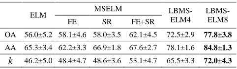
D. Contribution Analysis
Compared with ELM, the proposed MSELM features two contributions points, the feature extraction (FE) and sparse representation (SR). The LBMSELM are the improvement of MSELM incorporating the spectral information and spatial information. Hence, we will show the impact of each
contribution point in this subsection. We will use 10 samples per class (up to 50%) for training and the remaining for testing. Tables 1 and 2 show the classification accuracies in Indian Pines and Pavia University datasets, respectively, where OA, AA and k refer to the overall accuracy, average accuracy and the Kappa coefficient, respectively [50]. As seen from these tables, each contribution point has its improvement on ELM. Hence, we can conclude that the proposed MSELM and LBMSELM methods have outperformed ELM.
TABLE 1. CLASSIFICATION ACCURACY (%) AND STANDARD DEVIATION WITH 10 TRAINING SAMPLES PER CLASS FOR INDIAN PINES DATASET (BEST RESULTS
[image:7.612.324.566.201.271.2]IN BOLD).
TABLE 2. CLASSIFICATION ACCURACY (%) AND STANDARD DEVIATION WITH 10 TRAINING SAMPLES PER CLASS IN PAVIA UNIVERSITY DATASET (BEST
RESULTS IN BOLD).
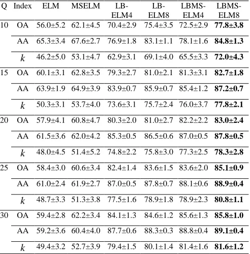
E. Effect of different numbers of training samples
In this subsection, we will compare the original ELM with the proposed MSELM and LBMSELM methods. We also apply the proposed local block method to ELM for comparison, i.e. local block ELMs including LBELM4 and LBELM8. We vary the number of the training samples Q randomly selected from each class, where Q=10, 15, 20, 25, 30 and capped to 50% of total pixels in each class in our experiments.
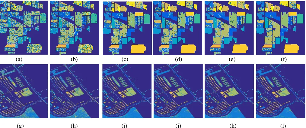
From the results in Tables 3 and 4, we can see an interesting phenomenon. With an increasing Q, the classification accuracy of ELM is decreasing for the Indian Pines dataset yet increasing at the beginning and then decreasing for the Pavia University dataset. This is caused by the ill-posed problem of ELM which can be seen from Fig. 4 (c) and (f), i.e., different numbers of hidden neurons are needed under varying number of training samples in order to achieve the optimal testing results. Fortunately, the proposed MSELM and LBMSELM methods alleviate this problem and can always produce significantly improved results. Fig. 5 shows the classification maps for the Indian Pines and Pavia University datasets with 30 training samples per class.
TABLE 3. CLASSIFICATION ACCURACY (%) AND STANDARD DEVIATION WITH DIFFERENT NUMBERS OF TRAINING SAMPLES IN INDIAN PINES DATASET (BEST
RESULTS IN BOLD)
Q Index ELM MSELM LB- ELM4
LB- ELM8
LBMS- ELM4
LBMS- ELM8 10 OA 50.1±1.2 63.1±3.1 66.8±2.5 70.0±2.3 75.2±3.0 77.2±2.6
ELM MSELM LBMS_
ELM4
LBMS- ELM8 FE SR FE+SR
OA 50.1±1.2 61.7±4.0 51.1±2.2 63.1±3.1 75.2±3.0 77.22±2.6 AA 62.2±1.6 70.5±3.4 63.6±2.7 71.9±2.1 84.8±1.3 86.43±1.0 k 44.4±1.5 56.9±4.3 45.5±2.6 58.4±3.5 72.1±3.3 74.36±2.9
ELM MSELM LBMS-
ELM4
LBMS- ELM8 FE SR FE+SR
[image:7.612.325.566.309.380.2]AA 62.2±1.6 71.9±2.1 79.4±1.0 82.0±1.0 84.8±1.3 86.4±1.0
k 44.4±1.5 58.4±3.5 62.8±2.7 66.4±2.5 72.1±3.3 74.3±2.9
15 OA 48.6±1.8 62.7±2.4 71.0±1.6 73.4±1.5 78.7±0.9 79.8±0.6
AA 59.7±2.0 71.8±1.6 83.2±0.9 84.8±0.9 87.5±0.6 88.7±0.6
k 42.6±2.1 58.0±2.7 67.6±1.8 70.2±1.7 76.0±1.0 77.2±0.6
20 OA 46.0±2.1 61.8±2.1 72.1±1.1 73.7±1.2 79.7±1.3 80.4±1.2
AA 56.8±2.3 70.8±1.5 84.8±0.7 85.9±0.6 89.0±0.4 89.5±0.2
k 39.8±2.5 56.8±2.5 68.8±1.1 70.5±1.3 77.2±1.3 77.9±1.3
25 OA 45.8±2.0 60.1±2.8 74.7±1.0 75.4±0.9 80.4±1.1 81.3±0.8
AA 55.4±1.6 68.3±2.1 86.4±0.7 87.1±0.6 89.5±0.7 90.1±0.6
k 39.4±2.0 55.0±3.1 71.6±1.1 72.3±1.0 77.9±1.2 78.8±0.9
30 OA 42.1±2.4 55.2±1.8 73.9±1.7 74.7±1.7 80.2±1.7 80.7±1.6
AA 50.5±2.7 63.4±2.8 86.3±1.0 87.1±0.9 89.7±0.9 90.1±0.8
k 35.0±2.6 49.3±2.1 70.7±1.8 71.6±1.8 77.7±1.8 78.3±1.7
TABLE 4. CLASSIFICATION ACCURACY (%) AND STANDARD DEVIATION WITH DIFFERENT NUMBERS OF TRAINING SAMPLES IN PAVIA UNIVERSITY DATASET
(BEST RESULTS IN BOLD).
Q Index ELM MSELM LB- ELM4
LB- ELM8
LBMS- ELM4
LBMS- ELM8 10 OA 56.0±5.2 62.1±4.5 70.4±2.9 75.4±3.5 72.5±2.9 77.8±3.8
AA 65.3±3.4 67.6±2.7 76.9±1.8 83.1±1.1 78.1±1.6 84.8±1.3
k 46.2±5.0 53.1±4.7 62.9±3.1 69.1±4.0 65.5±3.3 72.0±4.3
15 OA 60.1±3.1 62.8±3.5 79.3±2.7 81.0±2.1 81.3±3.1 82.7±1.8
AA 63.9±1.9 64.9±3.9 83.9±0.7 85.9±0.7 85.4±1.2 87.2±0.7
k 50.3±3.1 53.7±4.0 73.6±3.1 75.7±2.4 76.0±3.7 77.8±2.1
20 OA 57.9±4.1 60.8±4.7 80.3±2.0 81.0±2.7 82.2±2.2 83.0±2.4
AA 61.5±3.6 62.0±4.2 85.3±0.5 86.5±0.6 87.0±0.5 87.8±0.5
k 48.0±4.5 51.4±5.2 74.8±2.2 75.8±3.0 77.3±2.5 78.3±2.8
25 OA 58.4±3.0 60.6±3.4 82.4±1.4 83.6±1.5 83.6±2.0 85.1±0.9
AA 61.0±2.4 61.9±2.7 87.0±0.5 87.8±0.7 88.1±0.6 88.9±0.4
k 48.7±3.3 51.3±3.8 77.5±1.6 78.9±1.8 78.9±2.3 80.8±1.1
30 OA 59.4±2.8 62.2±3.4 84.1±1.3 84.6±1.2 85.6±1.3 85.8±1.0
AA 59.2±3.6 60.4±4.0 87.7±0.6 88.3±0.3 88.8±0.4 89.1±0.4
k 49.4±3.2 52.7±3.9 79.4±1.5 80.1±1.4 81.4±1.6 81.6±1.2
F. Comparison with state-of-the-art approaches
[image:8.612.46.292.51.265.2]In this subsection, we compare the proposed MSELM-LBP, LBMSELM4-LBP and LBMSELM8-LBP with state-of-the-art spectral and spatial methods, including LORSAL-SpATV [50], MASR [51] and LORSAL-LBP [41]. We also apply the LBP method to the original ELM for comparison. According to [41], we set the smooth parameter of LBP in Eq. (26) to 2. When applying the LBP to these methods, we only consider the labelled samples. About 1% of the total samples are used for training, and the remaining are used for testing. The details of training and testing samples in the Indian Pines and Pavia University datasets are summarized in Table 5.
TABLE 5. THE TRAINING/TESTING SAMPLES IN THE TWO DATASETS
Indian Pines Pavia University Index/category Train Test Index/Category Train Test 1 Alfalfa 3 51 1 Asphalt 66 6565 2 Corn-no till 14 1420 2 Meadows 186 18463 3 Corn-min till 8 826 3 Gravel 20 2079
4 Corn 4 230 4 Trees 30 3034
5 Grass/pasture 5 492 5 Metal sheets 13 1332 6 Grass/tree 8 739 6 Bare soil 50 4979 7 Grass/pasture-mowed 3 23 7 Bitumen 13 1317 8 Hay-windrowed 5 484 8 Bricks 37 3645
9 Oats 2 18 9 Shadows 10 937
10 Soybeans-no till 10 958 11 Soybeans-min till 24 2444 12 Soybeans-clean till 7 607
13 Wheat 4 208
14 Woods 13 1281 15 Bldg-grass-tree-drives 5 375 16 Stone-steel towers 4 91
Tables 6 and 7 show the classification results for the Indian Pines and Pavia University datasets, respectively, from which some useful conclusions can be summarized as follows. 1) Compared with ELM, the proposed MSELM, LBMSELM4 and LBMSELM8 all achieved better classification results, which have shown good performance of the proposed methods; 2) When applying LBP to ELM, MSELM and LBMSELM, the classification results can be further improved in terms of OA, AA and k. MSELM-LBP has similar classification results compared with ELM-LBP, but the combination of LBP with LBMSELM, i.e. LBMSELM4-LBP and LBMSELM8-LBP, have much better classification results than ELM-LBP. This verifies the merit of the proposed LBMSELM approach;
3) In comparison to other state-of-the-art methods, both LBMSELM4-LBP and LBMSELM8-LBP have achieved better classification results than LORSAL-SpATV, MASR and LORSAL-LBP. Figs. 6 and 7 show the classification maps of these methods with 1% samples used for training.
In the last row of Tables 6 and 7, we also give the running time of these methods for comparison. Tr and Ts denote the training time and testing time, respectively, measured in seconds (‘s’). Note that although the proposed LBMSELM is the development of MSELM, the former has less computation time than the latter in these tables. This is caused by different numbers of the hidden neurons L used for these two methods, where L is set to 250 and 1000 for LBMSELM and MSELM, respectively. As seen from Eqs. (16) and (20), both of the proposed MSELM and LBMSELM are iteration algorithms, which need the inverse operation with a size of L×L. With a much larger L used in MSELM than LBMSELM, the computational complexity of LBMSELM becomes less than that of MSELM.
[image:8.612.52.298.314.564.2]of these individual methods. In Table 7, the proposed LBMSELM4-LBP, LBMSELM8-LBP and MSELM-LBP have much more computation time than LRSAL-SpATV and MASR. In Table 6, LBMSELM4-LBP, LBMSELM8-LBP and MSELM-LBP methods have more computation time than LORSAL-SpATV, but slightly less computation time than MASR. These have again validated the good performance of the proposed approaches.
As a spatial-spectral classifier, LBMSELM seems to be sensitive to the spatial neighborhood used. We further evaluate the performance in terms of OA and computation time under varying size of neighborhoods. Tables 8 and 9 show the results
from the Indian Pines and Pavia University datasets, again using 10 labeled samples per class for training and the remaining for testing. As seen, the classification accuracy first increases, and soon saturates and even decreases with the enlarged neighborhood. That is because the spatial correction of pixels only holds within a small local area, and a too large neighborhood will inevitably degrade the results. Moreover, a larger neighborhood will naturally lead to more computation time in both training and testing. As a good tradeoff, we recommended 8 or 24 neighbors for a window size of 3×3 or 5×5 respectively for the proposed LBMSELM approaches.
(a) (b) (c) (d) (e) (f)
[image:9.612.54.561.204.417.2](g) (h) (i) (j) (k) (l)
Fig. 5. Results for the Indian Pines (up) and Pavia University dataset (down) (with 30 training samples per class) in terms of OA for (a) ELM (42.18±2.43); (b) MSELM (55.20±1.83); (c) LBELM4 (73.90±1.71); (d) LBELM8 (74.74±1.71); (e) LBMSELM4 (80.22±1.72); (f) LBMSELM8 (80.74±1.60); (g) ELM (59.44±2.82); (h) MSELM (62.27±3.41); (i) LBELM4 (84.13±1.32); (j) LBELM8 (84.66±1.20); (k) LBMSELM4 (85.65±1.37); and (l) LBMSELM8 (85.80±1.09).
(a) (b) (c) (d) (e) (f)
(g) (h) (i) (j) (k) (l)
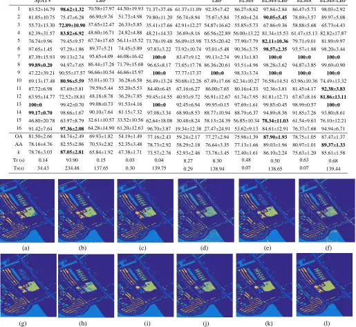
Fig. 6. Results for the Indian Pines dataset (~1% training), and the OAs are (a) LORSAL-SpATV (81.50±2.66); (b) MASR (84.74±2.49); (c) LORSAL-LBP (69.93±1.82); (d) ELM (54.19±1.49); (e) ELM-LBP (77.16±2.43); (f) MSELM (59.24±2.17); (g) MSELM-LBP (77.27±2.94); (h) LBMSELM4 (75.98±1.39); (i) LBMSELM4-LBP (87.90±1.93); (j) LBMSELM8 (78.75±1.05) (k) LBMSELM8-LBP (87.47±1.37); and (l) ground truth.
[image:9.612.54.554.461.677.2]SpATV LBP LBP ELM4 ELM4-LBP ELM8 ELM8-LBP
1 83.52±16.79 98.62±1.32 70.58±17.97 44.50±19.93 71.37±37.46 61.37±11.09 92.35±7.42 86.27±8.62 97.84±2.84 86.47±5.73 98.03±2.92
2 81.85±10.75 75.47±6.28 66.90±9.76 51.73±4.98 79.80±11.20 56.74±8.94 75.67±5.84 75.60±4.24 90.05±5.45 78.69±3.57 89.97±5.08
3 55.73±13.30 72.89±10.90 37.65±12.47 26.33±5.85 35.41±17.66 42.91±12.27 54.87±16.62 55.85±5.73 67.86±9.36 58.88±5.68 65.73±4.43
4 62.39±31.57 83.82±6.92 48.60±16.71 24.82±4.88 48.21±14.33 36.69±8.16 66.56±22.89 56.00±13.22 81.34±15.53 61.47±15.13 82.82±17.87
5 76.74±9.96 79.45±9.57 67.74±17.65 56.11±15.52 73.78±19.48 56.09±15.98 73.55±20.42 77.90±7.79 82.11±10.36 79.71±9.01 81.89±9.97
6 97.65±1.45 97.29±1.86 89.37±5.21 74.45±5.89 97.83±3.22 73.92±10.74 93.01±5.48 90.36±3.75 98.57±2.35 93.57±1.88 98.20±3.44
7 87.39±15.93 99.13±2.74 95.65±4.09 46.08±16.42 100±0 83.47±9.12 99.13±2.74 99.13±1.83 100±0 100±0 100±0
8 99.89±0.20 94.97±7.65 86.44±17.26 71.79±15.68 96.63±8.17 73.65±17.78 86.36±20.61 93.51±4.96 98.28±3.62 94.87±3.85 99.69±0.90
9 47.22±39.21 90.55±17.57 96.66±10.54 46.66±15.97 100±0 77.77±17.37 100±0 98.33±3.74 100±0 100±0 100±0
10 69.13±17.48 80.96±5.59 55.01±10.73 36.28±6.58 56.49±13.24 50.68±12.26 67.49±17.66 62.34±10.27 76.58±14.51 63.96±10.36 74.49±13.32
11 87.72±6.98 87.69±5.81 79.59±5.44 55.20±5.53 84.40±6.45 67.16±6.27 86.00±7.65 80.16±4.33 92.36±3.81 81.45±4.17 92.38±3.83
12 63.95±14.77 72.52±18.81 48.18±8.78 36.29±7.85 59.45±14.55 40.93±9.72 56.91±12.67 61.74±7.95 81.81±12.71 67.67±8.16 81.86±13.11
13 100±0 99.42±0.70 99.08±0.73 91.53±4.16 100±0 92.45±6.94 99.95±0.15 97.69±1.61 99.85±0.45 98.99±0.57 100±0
14 99.17±0.70 98.66±1.67 90.10±7.64 81.15±7.32 97.08±3.34 68.90±8.53 88.77±10.94 88.79±6.37 94.89±8.36 91.85±7.26 93.80±8.61
15 46.80±20.78 63.97±8.79 32.61±10.57 33.52±10.56 62.64±18.08 30.48±8.24 58.13±24.39 56.85±10.34 78.34±11.03 61.54±9.63 76.10±12.21
16 91.42±7.64 97.36±2.08 64.28±14.90 61.20±12.63 96.70±3.87 19.34±12.38 27.47±24.91 53.62±9.13 84.61±12.91 76.37±7.68 94.94±6.71
OA 81.50±2.66 84.74±2.49 69.93±1.82 54.19±1.49 77.16±2.43 59.24±2.17 77.27±2.94 75.98±1.39 87.90±1.93 78.75±1.05 87.47±1.37
AA 78.16±4.76 82.55±2.86 70.53±2.82 52.35±3.48 78.73±2.92 58.29±2.18 76.64±3.35 77.13±1.66 89.03±1.96 80.97±1.01 89.37±1.33
k 78.76±3.03 87.05±2.81 65.84±1.92 47.38±1.71 73.57±2.76 52.93±2.46 73.78±3.45 72.40±1.61 86.10±2.24 75.63±1.20 85.61±1.58
Tr (s) 0.14 93.90 0.15 0.03 0.04 8.27 8.30 0.48 0.50 0.63 0.68
Ts(s) 34.43 234.48 137.65 0.30 139.75 0.29 138.94 0.07 138.65 0.07 139.44
(a) (b) (c) (d) (e) (f)
[image:10.612.48.563.55.528.2](g) (h) (i) (j) (k) (l)
Fig. 7. Results for the Pavia University dataset (~1% training), and the OAs are (a) LORSAL-SpATV (93.19±1.58); (b) MASR (90.29±0.67); (c) LORSAL-LBP (93.02±0.60); (d) ELM (67.97±2.81); (e) ELM-LBP (89.71±1.81); (f) MSELM (70.16±2.54); (g) MSELM-LBP (89.74±1.62); (h) LBMSELM4 (89.68±0.46); (i) LBMSELM4-LBP (93.85±1.04); (j) LBMSELM8 (89.63±0.30) (k) LBMSELM8-LBP (93.60±0.89); and (l) ground truth.
TABLE 7. CLASSIFICATION ACCURACY (%) AND STANDARD DEVIATION WITH 1% TRAINING SAMPLES FOR PAVIA UNIVERSITY DATASET (BEST RESULTS IN BOLD). No. LORSAL-
SpATV MASR
LORSAL-
LBP ELM ELM-LBP MSELM
MSELM- LBP
LBMS- ELM4
LBMSELM4-LBP
LBMS ELM8
[image:10.612.60.562.570.737.2]Tr (s) 0.37 472.70 0.56 0.16 0.16 9.30 9.30 0.85 0.85 1.25 1.25
[image:11.612.341.537.176.315.2]Ts (s) 198.55 860.87 3748.4 1.02 3747.3 1.02 3759.2 0.25 3749.4 0.26 3749.9
TABLE 8. THE EFFECT OF THE SIZES OF THE NEIGHBORHOOD USED IN LBMSELM FOR THE INDIAN PINES DATASET
TABLE 9. THE EFFECT OF THE SIZES OF THE NEIGHBORHOOD USED IN LBMSELM FOR THE PAVIA UNIVERSITY DATASET
G. Comparing with Other Spatial Features and Deep Learning
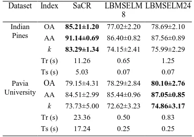
In Table 10, we compare the proposed LBMSELM (LBMSELM8 and LBMSELM 24) with the well-known spatial-aware collaborative representation (SaCR) approach [52] with 10 training samples per class, where the default parameters are adopted. For the Indian Pines dataset, SaCR has outperformed LBMSELM8 and LBMSELM24 in terms of classification accuracy. For the Pavia University dataset, SaCR has higher classification accuracy than LBMSELM8 yet lower than LBMSELM24. In both datasets, SaCR consumes much higher computational time that the proposed LBMSELM8 and LBMSELM24 approaches.
In addition, other spatial features including local binary pattern (LBPn) [28] and attribute profile (AP) [11] are compared with the proposed LBMSELM, where the default settings of parameters are used for these two approaches. With 1% labeled samples for training and the remaining for testing, the experimental results are reported in Tables 11 and 12 for comparison. When applying the AP to the proposed MSELM, the number of hidden neurons L is set to 1000 and 250 for the Indian Pines and Pavia University datasets, respectively. As seen from Tables 11 and 12, applying LBPn and AP to the proposed MSELM can further improve the classification accuracy. However, both LBPn-MSELM and AP-MSELM are still inferior than the proposed LBMSELM8, which indicates the efficacy of the spatial features extracted from LBMSELM8 than that of LBPn and AP.
In Table 13, we further compare the proposed MSLEM and LBMSELM8 with deep-learning based methods, including the convolutional neural networks (CNN) [53], CNN-pixel-pair features (CNN-PPF) [54] and Contextual Deep CNN (CD-CNN) [55]. Following the settings in [56], we set the training samples to 50 per class in both Indian Pines and Pavia University datasets and the remaining for testing. For consistency, only the 8 largest classes in Indian Pines dataset are used [55], corresponding to the 2nd, 3rd, 5th, 8th, 10th 11th, 12th and 14th classes as shown in Table 5. The classification results of CNN, CNN-PPF and CD-CNN are directly taken from [56]. We set the numbers of hidden neurons L to 100 and 900 for MSELM and LBMSELM8, respectively. For the Indian Pines dataset, LBMSELM8 outperforms all three deep-learning based approaches, although they have better results than the
proposed MSELM approach. For the Pavia University Dataset, CD-CNN produces the best result, yet our proposed LBMSELM8 outperforms two other deep-learning based approaches, i.e. CNN and CNN-PPF. This has again validated the good performance of the proposed LBMSELM8 method.
TABLE 10. CLASSIFICATION ACCURACY (%) AND STANDARD DEVIATION FOR INDIAN PINES AND PAVIA UNIVERSITY DATASETS (10 TRAINING SAMPLES PER
CLASS, BEST RESULTS IN BOLD).
Dataset Index SaCR LBMSELM 8
LBMSELM24
Indian Pines
OA 85.21±1.20 77.02±2.20 78.69±2.10
AA 91.14±0.69 86.40±0.82 87.56±0.89
k 83.29±1.34 74.15±2.41 75.99±2.29
Tr (s) 11.26 0.65 1.25
Ts (s) 5.03 0.07 0.07
Pavia University
OA 79.15±4.31 78.29±2.84 80.10±2.76
AA 84.51±2.99 85.44±0.96 87.05±0.85
k 73.73±5.00 72.62±3.23 74.86±3.17
Tr (s) 23.36 0.50 0.83
Ts (s) 17.24 0.25 0.25
H. Extended Experiments on the Salinas Dataset and Full Scene Classification Maps for the Three Datasets
In this subsection, we conduct more experiments to show the good performance of the proposed MSELM and LBMSELM on the Salinas dataset. Besides, we show the full scene classification maps for the three HSIs datasets used in our experiments. Salinas was also recorded by the AVIRIS sensor over the area surrounding the Salinas Valley, California. The spatial dimension of this dataset is 512×217 with 204 bands after removing 20 water absorption spectral bands [9]. Seventeen reference classes for 54129 labelled samples are available for classification in this dataset.
For the Salinas dataset, we select 10 samples per class for training and the remaining for testing, and the experimental results are compared in Table 14. The numbers of the hidden neurons L are set to 1000 for ELM and MSELM, and 250 for LBMSELM4 and LBMSELM8. Also, the parameter 𝐶 in Eq. (11) is set to 1000 for MSLEM, LBMSELM4 and LBMSELM8 As seen from Table 14, MSELM has better classification accuracy than ELM, whilst LBMSELM4 and LBMSELM8 have even better results than MSELM.
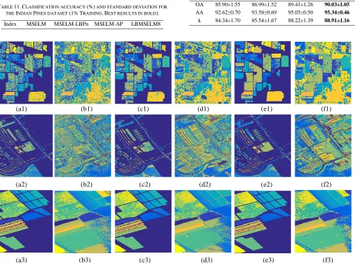
In Fig. 8, we show the full scene classification maps of ELM, MSELM and LBMSELM8 with 10 training samples per class for the three datasets, i.e. Indian Pines, Pavia University and Salinas. As seen from Fig. 8, the proposed MSELM and LBMSELM8 have much better classification results than ELM. Hence, the proposed methods have good performance.
V. CONCLUSION
In this paper, a novel framework based on multilayer optimization for ELM, MSELM, has been proposed to extract effective features and classify HSIs. By constructing the multilayer sparse ELM which extracts the effective feature and solves the ill-posed problem of ELM, the proposed MSELM
Index 4 8 24 48 80
OA 75.48±2.75 77.33± 2.34 78.90±2.18 78.75±1.81 78.18±1.77
Tr (s) 0.56 0.76 1.34 2.40 3.64
Ts (s) 0.07 0.08 0.07 0.08 0.07
Index 4 8 24 48 80
OA 72.58±2.09 78.08±3.10 80.02± 2.70 79.63±2.60 79.08±2.54
Tr (s) 0.41 0.52 0.83 1.43 2.08
[image:11.612.45.284.193.245.2]can greatly improve the classification results of ELM. Furthermore, a local block method that can reveal the neighboring information has been proposed to further improve the classification results of the MSELM. Finally, we apply the LBP to the proposed MSELM and LBMSELM, which can utilize the rich spectral and spatial information of HSIs. Compared with other state-of-the-art methods, the proposed methods obtain the good performances.
[image:12.612.320.559.51.86.2]In addition, the proposed methods can also be extended to many other HSIs applications such as target detection and anomaly detection. This is because these two applications can both be easily converted to a classification problem, where the proposed feature extraction and classification scheme can be applied. For the future work, we will resort to some mathematical methods, such as inverse free [57] to improve the computational efficiency of the proposed MSELM, LBMSELM method and LBP. Besides, we will also further improve the classification accuracy by using gravitational search [58] and saliency detection [59] approaches.
TABLE 11. CLASSIFICATION ACCURACY (%) AND STANDARD DEVIATION FOR THE INDIAN PINES DATASET (1% TRAINING, BEST RESULTS IN BOLD).
Index MSELM MSELM-LBPn MSELM-AP LBMSELM8
OA 58.87±3.24 69.34±3.38 69.90±5.12 78.71±1.10
AA 57.51±3.41 72.07±2.67 69.38±5.60 80.88±0.97
[image:12.612.321.556.121.169.2]k 52.52±3.65 65.04±3.78 65.33±6.01 75.58±1.24
TABLE 12. CLASSIFICATION ACCURACY (%) AND STANDARD DEVIATION FOR THE PAVIA UNIVERSITY DATASET (1% TRAINING, BEST RESULTS IN BOLD).
Index MSELM LBPa-MSELM AP-MSELM LBMSELM8
OA 70.26±2.70 75.83±2.26 83.51±0.97 89.69±0.32
AA 52.67±2.59 61.90±3.92 68.03±1.49 81.74±0.64
k 60.27±3.52 67.72±2.96 77.87±1.29 86.07±0.44
TABLE 13. CLASSIFICATION ACCURACY (%) AND STANDARD DEVIATION FOR INDIAN PINES AND PAVIA UNIVERSITY DATASETS (50 TRAINING SAMPLES,
BEST RESULTS IN BOLD).
Dataset Index CNN CNN-PPF CD-CNN MSELM LBMSELM8 Indian Pines OA 80.43 88.34 84.43 79.18 ±0.62 89.31 ±0.51 Pavia University OA 86.39 88.14 92.19 81.69±1.70 89.47±0.80
TABLE 14. CLASSIFICATION ACCURACY (%) AND STANDARD DEVIATION FOR THE SALINAS DATASET (10 TRAINING SAMPLES, BEST RESULTS IN BOLD).
(a1) (b1) (c1) (d1) (e1) (f1)
(a2) (b2) (c2) (d2) (e2) (f2)
(a3) (b3) (c3) (d3) (e3) (f3) Fig. 8. Results for the three datasets of Indian Pines (up), Pavia University (middle) and Salinas (bottom) with 10 training samples per class. In each row, a-b are for results from ELM, c-d are from MSELM, and e-f are from LBMSELM8. In addition, a, c and e are classification maps and b, d and f are full scene classification maps.
REFERENCES
[1] Y. Zhou, J. Peng, C.L.P. Chen, “Dimension reduction using spatial and spectral regularized local discriminant embedding for hyperspectral image
classification,” IEEE Trans. Geosci. Remote Sens. vol. 53, no. 2, pp. 1082-1095, 2015.
[2] L. Fang, S. Li, X. Kang, et al, “Spectral–spatial classification of hyperspectral images with a superpixel-based discriminative sparse Index ELM MSELM LBMSELM4 LBMSELM8
[image:12.612.54.565.287.665.2]model,” IEEE Trans. Geosci. Remote Sens. vol. 53, no. 8, pp. 4186-4201, 2015.
[3] X. Kang, P. Duan, S. Li, and J. A. Benediktsson, “Decolorization-based hyperspectral image visualization,” IEEE Trans. Geosci. Remote Sens., 2018.
[4] X. Kang, P. Duan, X. Xiang, S. Li, and J. A. Benediktsson, “Detection and correction of mislabeled training samples for hyperspectral image classification,” IEEE Trans. Geosci. Remote Sens., 2018.
[5] A. Plaza, J.A. Benediktsson, J.W. Boardman, et al., “Recent advances in techniques for hyperspectral image processing,” Remote Sens. Environ. vol. 113, no. 1, pp. S110-S122, 2009.
[6] Hughes, G, “On the mean accuracy of statistical pattern recognizers,” IEEE Trans. Inf. Theory. vol. 14, pp. 55-63, 1968.
[7] T. Qiao, Z. Yang, J. Ren, et al, “Joint bilateral filtering and spectral similarity-based sparse representation: A generic framework for effective feature extraction and data classification in hyperspectral imaging,” Pattern Recognit. vol. 77, pp. 316-328, 2018.
[8] H. Yu, L. Gao, J. Li, et al, “Spectral-spatial hyperspectral image classification using subspace-based support vector machines and adaptive Markov random fields,” Remote Sens. vol. 8, no. 4, pp. 355, 2016. [9] L. Fang, S. Li, W. Duan, J. Ren, J. A. Benediktsson, “Classification of
hyperspectral images by exploiting spectral-spatial information of superpixel via multiple kernels,” IEEE Trans. Geosci. Remote Sens. vol. 53, pp. 6663-6674, 2015.
[10] J. Li, J. M. Bioucas-Dias, A. Plaza, “Spectral–spatial hyperspectral image segmentation using subspace multinomial logistic regression and Markov random fields,” IEEE Trans. Geosci. Remote Sens. vol. 50, pp. 809-823, 2012.
[11] F. Cao, Z. Yang, J. Ren, W. K. Ling, H. Zhao, S. Marshall, “Extreme Sparse Multinomial Logistic Regression: A Fast and Robust Framework for Hyperspectral Image Classification,” Remote Sens. vo. 9, no. 12, pp.1255, 2017.
[12] F. Cao, Z. Yang, J. Ren, W.K. Ling, H. Zhao, M. Sun, J. A. Benediktsson, “Sparse Representation-Based Augmented Multinomial Logistic Extreme Learning Machine with Weighted Composite Features for Spectral-Spatial Classification of Hyperspectral Images,” IEEE Trans. Geosci. Remote Sens. vol. 56, no.11, pp. 6263- 6279, 2018.
[13] F. Cao, Z. Yang, J. Ren, M. Jiang, W. K. Ling, “Linear vs Nonlinear Extreme Learning Machine for Spectral-Spatial Classification of Hyperspectral Image,” Sensors. vol. 17, pp. 2603, 2017.
[14] J. Zabalza, J. Ren, Z. Liu, S. Marshall, “Structured covaciance principle component analysis for real-time onsite feature extraction and dimensionality reduction in hyperspectral imaging,” Appl. Opt. vol. 53, pp. 4440-4449, 2014.
[15] J. Zabalza, J. Ren, M. Yang, Y. Zhang, J. Wang, S. Marshall, J. Han, “Novel Folded-PCA for Improved Feature Extraction and Data Reduction with Hyperspectral Imaging and SAR in Remote Sensing,” ISPRS J. Photogramm. Remote Sens. vol. 93, pp. 112-12, 2014.
[16] X. Kang, X. Xiang, S. Li, and J. A. Benediktsson, “PCA-based edge-preserving features for hyperspectral image classification,” IEEE Trans. Geosci. Remote Sens., vol. 55, no. 12, pp. 7140–7151, 2017. [17] J. Zabalza, J. Ren, J. Zheng, H. Zhao, C. Qing, Z. Yang, P. Du, S. Marshall,
“Novel segmented stacked autoencoder for effective dimensionality reduction and feature extraction in hyperspectral imaging,”
Neurocomputing. vol. 185, pp. 1-10, 2016.
[18] T. Qiao, J. Ren, et al, “Effective denoising and classification of hyperspectral images using curvelet transform and singular spectrum analysis,” IEEE Trans. Geosci. Remote Sens. vol. 55, pp. 119-133, 2017. [19] J. Zabalza, J. Ren, J. Zheng, J. Han, H. Zhao, S. Li, S. Marshall, “Novel
two dimensional singular spectrum analysis for effective feature extraction and data classification in hyperspectral imaging,” IEEE Trans. Geosci. Remote Sens. vol. 53, pp. 4418-4433, 2015.
[20] T. Qiao, J. Ren, C. Craigie, J. Zabalza, C. Maltin, S. Marshall, “Singular spectrum analysis for improving hyperspectral imaging based beef eating quality evaluation,” Comput Electron Agric. vol. 115, pp. 21-25,2015. [21] G. B. Huang, Q. Y. Zhu, C. K. Siew, “Extreme learning machine: a new
learning scheme of feedforward neural networks,” Neural Networks, Proceedings. 2004 IEEE International Joint Conference on. IEEE, pp. 2: 985-990, 2004.
[22] Z. Bai, G. B. Huang, D. Wang, et al, “Sparse extreme learning machine for classification,” IEEE Trans. Cybern, vol. 44, no. 10, pp. 1858-1870, 2014.
[23] G. B. Huang, H. Zhou, X. Ding , et al, “Extreme learning machine for regression and multiclass classification,” IEEE Trans. Syst., Man, Cybern., Syst, vol. 42, no. 2, pp. 513-529, 2012.
[24] X. Liu, S. Lin, J. Fang, et al. “Is extreme learning machine feasible? A theoretical assessment (Part I),” IEEE Trans. Neural Netw. Learn. Syst, vol. 26, no. 1, pp. 7-20, 2015.
[25] S. Lin, X. Liu, J. Fang, et al, “Is extreme learning machine feasible? A theoretical assessment (Part II),” IEEE Trans. Neural Netw. Learn. Syst, vol. 26, no. 1, pp. 21-34, 2015.
[26] Q. Yu, Y. Miche, E. Eirola, et al, “Regularized extreme learning machine for regression with missing data,” Neurocomputing, vol. 102, pp. 45-51, 2013.
[27] L. L. C. Kasun, Y. Yang, G. B. Huang, et al, “Dimension reduction with extreme learning machine,” IEEE Trans. Image Process, vol. 25, no. 8, pp. 3906-3918, 2016.
[28] W. Li, C. Chen, H. Su, Q. Du, “Local binary patterns and extreme learning machine for hyperspectral imagery classification,” IEEE Trans. Geosci. Remote Sens, vol. 53, no. 7, pp. 3681-3693, 2015.
[29]C. Chen, W. Li, H. Su, et al, “Spectral-spatial classification of hyperspectral image based on kernel extreme learning machine,” Remote Sens., vol. 6, no. 6, pp. 5795-5814, 2014.
[30] F. Arguello, D.B. Heras, “ELM-based spectral–spatial classification of hyperspectral images using extended morphological profiles and composite feature mappings,” Int. J. Remote Sens., vol. 36, no. 2, pp. 645-664, 2015. [31]Y. Shen, J. Xu, H. Li, et al, “ELM-based spectral-spatial classification of
hyperspectral images using bilateral filtering information on spectral band-subsets,” in Proc. 2016 IEEE Int. Remote Sens. Symp. (IGARSS), Beijing, China, pp. 497-500, 2016.
[32] H. Su, S. Tian, Y. Cai, et al, “Optimized extreme learning machine for urban land cover classification using hyperspectral imagery,” Front. Earth Sci. vol. 11, no. 4, pp.765-773, 2017.
[33] B. Stephen, et al, "Distributed optimization and statistical learning via the alternating direction method of multipliers," Foundations and Trends in Machine learning, vol. 3, no. 1, pp. 1-122, 2011.
[34] Y. Chen, N. M. Nasrabadi, T. D. Tran, “Hyperspectral image classification using dictionary-based sparse representation,” IEEE Trans. Geosci. Remote Sens. vol. 49, no. 10, pp. 3973-3985, 2011.
[35] G. B. Huang, Q. Y. Zhu, C. K. Siew, “Extreme learning machine: theory and applications,” Neurocomputing, vol. 70, no. 1, pp. 489-501, 2006. [36] K.S. Banerjee, Generalized inverse of matrices and its applications, Wiley.
1971.
[37] C. Chen, “A rapid supervised learning neural network for function interpolation and approximation,” IEEE Trans. Neural Netw., vol. 7, no. 5, pp. 1220-1230, 1996.
[38] M. Afonso, J. Bioucas-Dias, M. Figueiredo, “Fast image recovery using variable splitting and constrained optimization,” IEEE Trans. Image Process., vol. 19, no. 9, pp. 2345-2356, 2010.
[39]J. Bioucas-Dias, M. Figueiredo, “Multiplicative noise removal using variable splitting and constrained optimization,” IEEE Trans. Image Process., vol. 19, no. 7, pp. 1720-1730, 2010.
[40] P. L. Bartlett, “The sample complexity of pattern classification with neural networks: the size of the weights is more important than the size of the network,” IEEE Trans. Inf. Theory, vol. 44, no. 2, pp. 525-536,1998. [41] J. Li, J. M. Bioucas-Dias, A. Plaza A, “Spectral–spatial classification of
hyperspectral data using loopy belief propagation and active learning,”
IEEE Trans. Geosci. Remote Sens.vol. 51, no. 2, pp. 844-856, 2013. [42] M. Fauvel, Y. Tarabalka, J. A. Benediktsson, et al, “Advances in
spectral-spatial classification of hyperspectral images. Proc. IEEE. vol. 101, pp. 652-675, 2013.
[43] Y. Tarabalka, M. Fauvel, J. Chanussot, et al, “SVM-and MRF-based method for accurate classification of hyperspectral images,” IEEE Geosci. Remote Sens. Lett. vol. 7, pp. 736-740, 2010.
[44] P. Ghamisi, J. A. Benediktsson, M. O. Ulfarsson, “Spectral-spatial classification of hyperspectral images based on hidden Markov random fields,” IEEE Trans. Geosci. Remote Sens., vol. 52, pp. 2565-2574, 2014. [45]F. Cao, Z. Yang, J. Ren, et al, “Convolutional neural network extreme
learning machine (CNN-ELM) for effective classification of hyperspectral images,” Journal of Applied Remote Sens., 12(3) 035003 2018.
millennium: Morgan Kaufmann Publishers Inc. San Francisco, CA, USA, pp. 236-239, 1-55860-811-7, 2003.
[47] J. S. Yedidia, W. T. Freeman, Y. Weiss, “Constructing free-energy approximations and generalized belief propagation algorithms,” IEEE Trans. Inf. Theory. vol. 51, pp. 2282-2312, 2005.
[48 J. Eckstein, D. P. Bertsekas, “On the Douglas—Rachford splitting method and the proximal point algorithm for maximal monotone operators,” Math. Program., vol. 55, no. 1, pp. 293-318, 1992,
[49] J. Li, X. Huang, P. Gamba, et al, “Multiple feature learning for hyperspectral image classification,” IEEE Trans. Geosci. Remote Sens, vol. 53, no. 3, pp. 1592-1606, 2015.
[50] L. Sun, Z. Wu, J. Liu, et al, “Supervised spectral–spatial hyperspectral image classification with weighted Markov random fields,” IEEE Trans. Geosci. Remote Sens., vol. 53, no. 3, pp. 1490-1503, 2015.
[51] L. Fang, S. Li, X. Kang, et al, “Spectral–spatial hyperspectral image classification via multiscale adaptive sparse representation,” IEEE Trans. Geosci. Remote Sens. vol. 52, no. 12, pp. 7738-7749, 2014.
[52] J. Jiang, C. Chen, Y. Yu, et al, “Spatial-aware collaborative representation for hyperspectral remote sensing image classification,” IEEE Geosci. Remote Sens. Lett, vol. 14, no.3, pp. 404-408, 2017.
[53] W. Hu, Y. Huang, L. Wei, et al, “Deep convolutional neural networks for hyperspectral image classification,” J. Sen, 2015, 2015.
[54] W. Li, G. Wu, F. Zhang, et al, “Hyperspectral image classification using deep pixel-pair features,” IEEE Trans. Geosci. Remote Sens, vol. 55, no. 2, pp. 844-853, 2017.
[55] H. Lee, H. Kwon, “Going deeper with contextual CNN for hyperspectral image classification,” IEEE Trans. Image Process, vol. 26, no. 10, pp. 4843-4855, 2017.
[56] M. Zhang, W. Li, Q. Du, “Diverse Region-Based CNN for Hyperspectral Image Classification,” IEEE Trans. Image Process, vol. 27, no. 6, pp. 2623-2634, 2018.
[57] S. Li, Z. H. You, H. Guo, et al, “Inverse-free extreme learning machine with optimal information updating,” IEEE Trans. Cybern. vol. 46, pp. 1229-1241, 2016.
[58] G. Sun, P. Ma P, J. Ren, et al, “A stability constrained adaptive alpha for gravitational search algorithm,” Knowl-Based. Syst., 2018, 139: 200-213 [59] Y. Yan, J. Ren, G. Sun, et al, “Unsupervised image saliency detection with
gestalt-laws guided optimization and visual attention based refinement,”