Lasing behavior of an active NIM-PIM DC with different coupling coefficients

(1)

Rochester Institute of Technology

RIT Scholar Works

Theses Thesis/Dissertation Collections

8-15-2012

Lasing behavior of an active NIM-PIM DC with

different coupling coefficients

Abdulaziz Atwiri

Follow this and additional works at:http://scholarworks.rit.edu/theses

This Thesis is brought to you for free and open access by the Thesis/Dissertation Collections at RIT Scholar Works. It has been accepted for inclusion in Theses by an authorized administrator of RIT Scholar Works. For more information, please contactritscholarworks@rit.edu.

Recommended Citation

(2)

Rochester Institute of Technology (RIT)

College of Applied Sciences and Technology (CAST)

Department of Electrical, Computer, and Telecommunication Engineering Technology (ECTET)

Lasing Behavior of an Active NIM-PIM DC

with Dierent Coupling Coecients

Abdulaziz S. A. Atwiri

August 15th 2012

Rochester, NY, USA

A Research Thesis are Submitted to Complete the Requirements

of the degree

(3)

Thesis Supervisor Professor

Dr.Drew N. Maywar

Department of Telecommunications Engineering Technology

College of Applied Sciences and Technology

Rochester Institute of Technology

Rochester, New York

Approved by:

...

Dr. Drew N. Maywar, Thesis Advisor

Department of Electrical and Telecommunications Engineering Technology.

...

Professor Michael Eastman, Department Chair

Department of Electrical and Telecommunications Engineering Technology.

...

Professor Mark J. Indelicato, Committee Member

(4)

Abstract

Metamaterials is a class of materials that do not exist naturally. This kind of material has interesting properties that dier from subclass to another and are researched for its numerous potential usages. One of these subclasses is negative index materials (NIMs). This subclass has special properties that make its refractive index negative. Trying to take advantage of this property in photonic structures has led to many new and interesting photonic structures that can be used in industry. One application that makes use of NIMs properties is the NIM-PIM DC. NIM-PIM DC, which is a photonic structure that is made of two parallel waveguides where one of them is made of PIM materials while the other one is made of NIM materials with a coupling region between them, can provide some new features to photonic circuits, and one of these features is optical feedback. So, it can be used in a photonic devices and components that need a feedback.

This thesis studies for the rst time the ability to manage and control the las-ing behavior of an active NIM-PIM DC by changlas-ing the coupllas-ing between the two waveguides. starting from coupled-mode equations considering the structure's limi-tations and conditions, the lasing governing equations have been derived, analyzed, and tested using mathematical forms and MATLAB plots. The governing equations that are studied here are eigen-value, transmittivity, and reectivity equations of a NIM-PIM DC structure.

(5)

Acknowledgment

All praise and thanks to God who creates me, makes me able to accomplish all my life's projects, and puts helpful people along my way to help me. Also, I would like to express my thanks to people who helped me through my academic life.

With sincere and no limitations, I would like to thank my thesis supervisor, Professor Drew N. Maywar. His patience, encouragement, help, and support have overcome diculties and made me able to complete my dierent thesis tasks.

(6)

CHAPTER 1 1 Introduction

1.1 Metamaterials

Metamaterials is a term used to refer to the materials that are articially engineered and containing nanostructures which give these structures specic and remarkable properties [1]. The term Meta itself has been given several meanings, and some of these meanings are altered changed and higher beyond. According to the above denitions of the prex Meta, people have several denitions that describe these structures, and when they are used together, give the reader a good imagine about it. Some of these denitions include:

• Any material that can have their electromagnetic properties altered to

some-thing beyond what can be found in nature.

• Any material composed of periodic macroscopic structures to achieve a desired

(9)

Structures that have metamaterials properties are usually made from two or more dierent materials and they are made to be periodic with a period being small com-paring to the wavelength of light that passes the structure. In physics, metamaterials

are the materials with negative or zero refractive index nr . This negative refractive

index can be achieved when both permittivity r and permeability µr are negative.

This combination of negative r and negative µr cannot be found naturally in any

material.

The rst metamaterial was used in the microwave spectrum, and the rst form of it relied on a combination of split-ring resonators (SRRs) and conducting wires.

SRRs were used to generate the desired µr and the conducting wires used to

gener-ate the desiredr . These days, metamaterials have become almost the hottest eld

of research in many scientic disciplinarians such as physics, optics, and photon-ics engineering. Their applications have shown success in dierent types of optical and microwave devices such as modulators, band-pass lters, lenses, couplers, split-ters, and antenna systems. Furthermore, the lower density and small size of these structures have promised to introduce lighter and smaller devices and systems while advancing and enhancing the overall performance.

(10)

arise from the properties of the materials itself. In particular, there are no perfect conductors for frequencies of hundreds of terahertz. Therefore, particularly devices for the highest frequencies exhibit relatively high optical losses.

Metamaterials are classied into six categories as follows:

• Negative index materials.

• Single negative metamaterials.

• Electromagnetic band-gap metamaterials.

• Double positive media.

• Bi-isotropic and bi-anisotropic metamaterials.

• Chiral metamaterials.

In this thesis, negative index metamaterials have been investigated and studied in some specic photonic structures.

1.2 Negative index materials (NIMs)

The NIM idea was rst introduced by a Russian physicist V. Veselago in 1967. The main key of this kind of material was how to get a special material with negative

refractive index nr [20]. To obtain such a material, you need it to have a negative

permittivityr and negative permeability µr at the same time. To have such r and

µr , you have to consider many characters that r and µr depend on, and some of

(11)

• Operating frequency.

• Propagation direction.

• Polarization state.

If both r and µr are negative (some people like to name it double-negative

meta-material), the refraction phenomenon at the interface between the vacuum and the material is dierent. The refracted beam is not in the usual side as the positive-index materials, the negative refractive index changes the sign of the angle in Snell's law. Fig. (1.1) shows the dierence between the positive-index and the negative-index materials in terms of refraction phenomenon.

Figure 1.1: Reection of light: positive-index and negative-index materials.

When a beam coming from vacuum hits a negative-index material (right side), the refracted beam inside the medium is on the same side of the surface normal as the in-cident beam. This is totally in contrast to the situation for ordinary positive-index materials (left side). The normal can be dened as an imaginary line perpendicular to the interface.

(12)

have placed it on the top of many research elds. Many applications that make use of NIMs has reported, and many others are under study and investigation, and some of these applications are:

• super-lens, reported by J. Pendry in 2000 [21].

• invisibility cloaks.

• optical nanolithography antennas with advanced properties of reception and

range.

1.3 NIM-PIM Directional Couplers

NIM-PIM DC is a photonic structure that consists of two parallel waveguides with a coupling region. It looks like an ordinary PIM-PIM DC with only one dierence in their structures. While the PIM-PIM DC consists of two identical positive-index wave guides, the NIM-PIM DC consists of a positive-index waveguide placed in parallel with a negative-index waveguide. This special structure changes the way that light usually acts in PIM-PIM DC. While the PIM-PIM DC introduces two forward output signals, the NIM-PIM DC introduces one forward and one backward output signal [11]. This property makes the NIM-PIM DC acts somehow like a regular DFB resonator. This property makes it usable as a feedback device or optical enhancement machine in some optical applications.

(13)

• Alu and Engheta reported (2005): Governing equations of a linear NIM-PIM

directional coupler.

• Litchinitser , Gabitov, and Maimistov reported (2007): Governing equations

of a nonlinear NIM-PIM directional coupler. Optical bistability.

• Ara and Maywar reported (2011): Lasing behavior of a NIM-PIM directional

coupler with optical gain introduced. Considered symmetric coupling strength between waveguides.

The present research is focused on how can this structure be used in some applications like optical memory, optical switching, optical routing, optical lters, and all optical digital signal processing.

1.4 Overview of Thesis

(14)

The other three chapters have been designed to discuss the following main topics respectively:

• Investigating, discussing, and understanding the main equations and behavior

of passive structures.

• Investigating, discussing, and understanding the main equations and behavior

of active structures.

• Investigating, discussing, and understanding the lasing behavior of active

struc-tures.

(15)

.

Chapter 2 2 Passive NIM-PIM DC with Dierent Coupling

2.1 Optical Waveguides and Coupled-Mode Theory

A specic structure that lies at the heart of the integrated photonic industry is called an optical waveguide. An optical waveguide is a spatially dierentiated structure that guides light in a way the manufacturer needs. This special guidance of light restricts propagation in specic directions within the boundaries of the structure [22]. This precious operation (the light guidance) is usually achieved by making a structure with a lower refractive index material usually called the cladding surrounding a higher refractive index material usually called the core, which means the designer make use of total internal refection.

(16)

classied as gradient and step-index waveguides. And based on their geometry, they can be classied as planar and channel waveguides. The planar and channel waveguides are shown in Fig. 2.1.

Figure 2.1: Types of waveguides based on their geometry.

There are many applications of optical waveguides, and some of these applications are:

• Optical ber used for communications.

• Photonic integrated circuits to guide light between dierent components.

• Digital processor chips in computer industries for future generation of super

fast computing.

• Frequency doublers, lasers, and optical ampliers.

• Splitter and/or combiner of light beams. [22]

(17)

Coupled-mode theory gives fairly accurate results, and it is extremely simpler than the old methods which concern applying Maxwell's equations with the boundary conditions. This thesis will investigate a system of channel waveguides of which their nal transmittivity and reectivity forms are derived from the coupled-mode theory.

The phenomena of perturbed elds, exchanging power, and their solution with coupled-mode theory have introduced the waveguide structure benets and have led to the innovation of many optical devices that are used nowadays and will be used in the future.

2.2 Passive PIM-PIM Directional Coupler

2.2.1 Directional Coupler

A directional coupler (DC) is a device that combines and/or separates light. A directional coupler is a four-port device that is made to have specic light intensity in specic ports. For example, a 3-dB directional coupler divides the input light equally to its two output ports. A directional coupler is usually made of two waveguides that are shaped and placed in a specic way to get specic results.

(18)

• Waveguide core diameter in the coupling region.

• The distance between the waveguide cores.

• The length of the coupling region.

• The pass-through light's wavelength.

Fig. 2.2 shows a 3-dB PIM-PIM DC which is widely used in ber-optic system components, and we will discover its main equations and solutions for its power exchange, its transmittivity, and its reectivity in the following section.

Figure 2.2: A 3dB PIM-PIM DC.

2.2.2 Coupled-Mode Equations and General Solution

There are two dierent sets of the coupled-mode equations1 _{for a passive PIM-PIM}

DC. The rst set assumes that we are using e−iωt _{for the time-dependent phasor,}

and this set can be written as [18]:

1_{More information about the coupled-mode equations, their conventions, basics, considerations,}

(19)

dEa(z)

dz =ikbae

−i4βz

Eb(z) (2.1)

dEb(z)

dz =ikabe

i4βz_E

a(z). (2.2)

The second set assumes that we are usinge+iωt for the time-dependent phasor, and

this set can be written as:

dEa(z)

dz =−ikbae

i4βz_E

b(z) (2.3)

dEb(z)

dz =−ikabe

−i4βz_E

a(z), (2.4)

where Ea and Eb represent the electrical eld of forward traveling modes in the A

and B waveguides, respectively, kab and kba represent the coupling coecient of the

waveguide A into the waveguide B and the coupling coecient of the waveguide B into the waveguide A, respectively.

4β =βa−βb, represents the detuning between the waveguides, whereβa

repre-sents the propagation number of waveguide A,βb represents the propagation number

of waveguide B, and the mathematical form of the propagation number β in

gen-eral is β = 2_λπ

on . n represents the modal refractive index, and λo represents the

wavelength in vacuum.

For our future work, we will stick to the rst set of the coupled-mode equations, and we will explain the dierences that may be found by using the second set in the appendix. For the rst set, the electrical eld for waveguide A and B is dened as:

(20)

EB(z) = Eb(z)ei(βbz−ωt).

First, we normalize the rst set by introducing the waveguide length l as the

follow-ing:

ldEa(z)

dz =ikbale

−i4βl_lz_E

b(z) (2.5)

ldEb(z)

dz =ikable

i4βl_lz_E

a(z). (2.6)

Now, let ζ = z_l, so equations (2.5) and (2.6) can be rewritten as:

dEa(ζ)

dζ =ikbale

−i4βlζ_E b(ζ)

dEb(ζ)

dζ =ikable

i4βlζ_E a(ζ).

Now, we introduce kab,kba, and4β as normalized forms ofkab, kba, and4β

respec-tively (where x=xl), the above two equations become:

dEa(ζ)

dζ =ikbae

−i4βζ_E

b(ζ) (2.7)

dEb(ζ)

dζ =ikabe

i4βζ_E

a(ζ). (2.8)

The two electromagnetic elds Ea(z) and Eb(z) can be dened as follows.

(21)

EA(z) = Ea(z)eiβaze−iωt. (2.9)

From our initial denition EA(z) in terms of β is:

EA(z) = Aeiβze−iωt, (2.10)

whereA is the eld amplitude in waveguide A, and β = βa+βb

2 .

Now, the left hand side of equations (2.9) and (2.10) are equal to each other which means that the right hand sides are equal to each other too. applying that yields:

Ea(z)eiβaz =Aeiβz.

Solving it for Ea(z) yields:

Ea(z) =Aei(β−βa)z. (2.11)

Now, from our previous denition,4β =βa−βb, and βb = 2β−βa, substituting the

value of βb into 4β equation yields:

4β =βa−2β+βa

β−βa=− 4β

2 .

Substituting the above equation into equation (2.11) yields:

Ea(z) =Ae−i

4β

(22)

For waveguide B, and from our initial denition EB(z)in terms of βb is:

EB(z) =Eb(z)eiβbze−iωt. (2.13)

From our initial denition EB(z)in terms of β is:

EB(z) =Beiβze−iωt, (2.14)

whereB is eld amplitute in waveguide B, and β = βa+βb

2 .

Now, the left hand side of equations (2.13) and (2.14) are equal to each other which means that the right hand sides are equal to each other too. applying that yields:

Eb(z)eiβbz =Beiβz.

Solving it for Ea(z) yields:

Eb(z) =Bei(β−βa)z. (2.15)

Now, from our previous denition,4β =βa−βb, and βa= 2β−βb, substituting the

value of βa into 4β equation yields:

4β = 2β−βb−βb

β−βb = 4β

2 .

Substituting the above equation into equation (2.15) yields:

Eb(z) = Bei

4β

(23)

Normalizing both equations (2.12) and (2.16) using the same l and ζ yields:

Ea(z) =Ae−i

4β

2 z

l l

Ea(ζ) = Ae−i

4β

2 lζ

Ea(ζ) = Ae−i

4β

2 ζ (2.17)

Eb(z) = Bei

4β

2 z

l l

Eb(ζ) =Bei

4β

2 lζ

Eb(ζ) =Bei

4β

2 ζ. (2.18)

Substituting equations (2.17) and (2.18) into equation (2.7), and solving the new equation yields:

dAe−i4₂βζ

dζ =ikbae

−i4βζ_Bei4₂βζ

dA dζ

e−i42βζ

+A

−i4β

2

e−i42βζ =ik_baBe−i

4β

2 ζ

dA dζ +A

−i4β

2

(24)

dA dζ =i

4β

2 A+ikbaB. (2.19)

dBei4₂βζ

dζ =ikabe

i4βζ_Ae−i4₂βζ

dB dζ

ei42βζ

+B

i4β

2

ei42βζ =ik_abAei

4β

2 ζ

dB dζ +B

i4β

2

=ikabA

dB dζ =−i

4β

2 B+ikabA. (2.20)

The two dierential equations (2.19) and (2.20) are the main equations that describe the behavior of PIM-PIM DC, and their general solutions can be dened as:

A(z) = A1eiqz +A2e−iqz

B(z) = B1eiqz +B2e−iqz,

where q represents the unknown eigen-value, and normalizing the above two

equa-tions by introducing the waveguide length l yields:

(25)

B(ζ) =B1eiqζ+B2e−iqζ (2.22)

where q=qlis the normalized eigen-value, and A1, A2, B1,and B2 are constants.

2.2.3 Dispersion Relation and Eigenvalue

Substituting both equations (2.21) and (2.22) into equation (2.19) yields:

d dζ A1e

iqζ₊_A 2e−iqζ

=i4β

2 A1e

iqζ₊_A 2e−iqζ

+ikba B1eiqζ +B2e−iqζ

A1(iq)eiqζ +A2(−iq)e−iqζ =i 4β

2 A1e

iqζ ₊_A 2e−iqζ

.

Equating the terms that haveeiqζ yields:

A1(iq)eiqζ =i 4β

2 A1e iqζ

+ikba B1eiqζ

q−4β 2

A1 =kbaB1. (2.23)

Equating the terms that havee−iqζ yields:

A2(−iq)e−iqζ =i 4β

2 A2e

−iqζ

+ikba B2e−iqζ

q+4β 2

A2 =−kbaB2. (2.24)

(26)

d dζ B1e

iqζ₊_B 2e−iqζ

=−i4β

2 B1e

iqζ ₊_B 2e−iqζ

+ikab A1eiqζ+A2e−iqζ

B1(iq)eiqζ +B2(−iq)e−iqζ =−i 4β

2 B1e

+ikab A1eiqζ+A2e−iqζ

.

B1(iq)eiqζ =−i 4β

2 B1e iqζ

+ikab A1eiqζ

q+4β 2

B1 =kabA1. (2.25)

B2(−iq)e−iqζ =−i 4β

2 B2e

−iqζ

+ikab A2e−iqζ

q−4β 2

B2 =−kabA2. (2.26)

Either way, substituting equation (2.25) into equation (2.23) or substituting equation

(2.26) into equation (2.24) gives us the value of the eigen-value q.

From equation (2.25), B1 can be written as:

B1 =

kab

q+4₂β

(27)

q− 4β 2

A1 =kba

kab

q+4₂β

A1

q2 =

4β

2

+kabkba

q =±

s

₄

β

2

+kabkba. (2.27)

2.2.4 Boundary Conditions and Specic solution

We assume that the light pulse is launched only in waveguide A, which means that

no light energy or any kind of light pulses enter waveguide B at ζ = 0. Thus

B(ζ = 0) = 0. Using this value in equation (2.22) yields:

B(ζ) =B1eiqζ+B2e−iqζ

0 = B1+B2

B2 =−B1. (2.28)

Substituting equation (2.28) into equation (2.22) yields:

(28)

Using Euler's formulasin(x) = eix−₂e_i−ix yields:

B(ζ) = i2B1sin(qζ). (2.29)

dB dζ =−i

4β

2 B+ikabA

d

dζ(i2B1sin(qζ)) = −i

4β

2 (i2B1sin(qζ)) +ikabA

2B1

d

dζ(sin(qζ)) = −i

4β

2 (2B1sin(qζ)) +kabA

2B1qcos(qζ) =−i 4β

2 (2B1sin(qζ)) +kabA

kabA= 2B1qcos(qζ) +i 4β

2 (2B1sin(qζ)).

Solving the above equation for A yields:

A(ζ) = 2B1

kab

qcos(qζ) +i4β

2 sin(qζ)

. (2.30)

2.2.5 Power Exchange - Output Ports

Using equation (2.30) and our assumption that the launched power only exists in

(29)

A(ζ) = 2B1

kab

qcos(qζ) +i4β

2 sin(qζ)

A(ζ = 0) = 2B1

kab

q (2.31)

Pi =|A(ζ = 0)|2 =

2B1

kab

2

|q|2.

Now, let us say that PA is the power in waveguide A, that yields:

PA=|A(ζ)| 2

PA=Pi

cos(qζ) +i4β

2q sin(qζ)

2

.

Using equation (2.29), the eld in waveguide B can be written as follows:

B(ζ) =i2B1sin(qζ)

atζ = 0

B(0) =i2B1sin(0) = 0

atζ = 1

B(ζ = 1) =i2B1sin(q).

(30)

PB =|B(ζ)|2 =Pikab 2

isin(qζ)

q

2

.

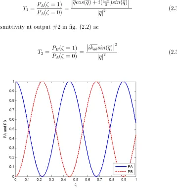
From above discussion, we can write the transmittivity at two output ports of two

waveguides as follows: T1 the transmittivity at output #1 in g. (2.2) is:

T1 =

PA(ζ = 1)

PA(ζ = 0) =

qcos(q) +i(

4β

2 )sin(q)

2

|q|2 (2.32)

T2 the transmittivity at output #2 in g. (2.2) is:

T2 =

PB(ζ = 1)

PA(ζ = 0) =

ikabsin(q)

2

[image:30.612.156.514.204.586.2]

|q|2 (2.33)

Figure 2.3: The power exchange between the two waveguides of a PIM-PIM DC

As clearly shown in g. (2.3), at ζ = 0, PA represents the total input power and

PB = 0 . Also, atζ = 1, The place where the PIM-PIM DC structure has its output

(31)

of a 3-dB structure]. Changing4β allows us to change the output powers in a way that we can set any ratio of the input power to any output port of the device. I

mean the ability to get from 0% to 100% of the output power in any output port

you need.

2.3 Passive NIM-PIM Directional Coupler

2.3.1 Directional Coupler

In this whole section, we will rediscuss what we have discussed in section (2.2), and we will seek the same things like eigen-value, the power in two waveguides, transmit-tivity, and reectivity of the system. The only dierence and the big dierence here is the second waveguide in our directional coupler. While in section (2.2) we employ a directional coupler with two positive index materials waveguides, in this section, we will employ a directional coupler with two dierent waveguides. One of them is made of a positive index material, whereas the second one is made of a negative index material which called Metamaterial.

The following subsection investigates in detail the coupled-mode equations and their solutions for this case. But to have this system in a glance, it looks like g. (2.4).

(32)

Following the same strategy that we dened in section (2.2.2), we will nd two dierent sets of the coupled-mode equation for a passive NIM-PIM DC. Sticking with the same path we already chose, our denition for the electromagnetic eld

using e−iωt for the time-dependent phasor will stay the same. This denition yields

the following set of coupled-mode equations for NIM-PIM DC [11]:

dEa(z)

dz =ikbae

−i4βz_E

b(z) (2.34)

dEb(z)

dz =−ikabe

i4βz_E

a(z), (2.35)

where Ea and Eb represent the electrical eld of forward and backward traveling

modes, respectively, kab and kba represent the coupling coecient of the waveguide

A into the waveguide B and the coupling coecient of the waveguide B into the

waveguide A, respectively, 4β represents the detuning between the waveguides.

4β = βa−βb, where βa represents the propagation number of the waveguide

A,βb represents the propagation number of the waveguide B, and the mathematical

form of the propagation number β in general is β = 2_λπ

on , where n represents the

modal refractive index, and λo represents the wavelength in the air.

Following the same strategy to normalize the rst set of coupled-mode equations yields:

dEa(ζ)

dζ =ikbae

−i4βζ

Eb(ζ) (2.36)

dEb(ζ)

dζ =−ikabe

i4βζ_E

(33)

whereζ = z_l, and kab,kba, and 4β are normalized forms ofkab, kba, and 4β

respec-tively, wherex=xl.

The two electromagnetic elds Ea(z) and Eb(z) can be dened as follows:

Ea(z) = Ae−i

4β

2 z (2.38)

Eb(z) = Bei

4β

2 z. (2.39)

Normalizing both elds using the samel and ζ yields:

Ea(ζ) = Ae−i

4β

2 ζ (2.40)

Eb(ζ) =Bei

4β

2 ζ. (2.41)

dAe−i4₂βζ

dζ =ikbae

−i4βζ_Bei4₂βζ

dA dζ

e−i42βζ

+A

−i4β

2

e−i42βζ =ik_baBe−i

4β

2 ζ

dA dζ +A

−i4β

2

=ikbaB

dA dζ =i

4β

(34)

dBei4₂βζ

dζ =−ikabe

i4βζ_Ae−i4₂βζ

dB dζ

ei42βζ

+B

i4β

2

ei42βζ =−ik_abAei

4β

2 ζ

dB dζ +B

i4β

2

=−ikabA

dB dζ =−i

4β

2 B −ikabA

−dB

dζ =i

4β

2 B+ikabA. (2.43)

The two dierential equations (2.36) and (2.37) are the main equations that describe the behavior of NIM-PIM DC, and their general solutions can be dened as:

A(z) = A1eiqz +A2e−iqz

B(z) = B1eiqz +B2e−iqz,

where q represents the unknown eigen-value, and normalizing the above two

equa-tions by introducing the waveguide length l yields:

(35)

B(ζ) = B1eiqζ +B2e−iqζ, (2.45)

where q=ql, and it represents the normalized eigen-value

d dζ A1e

iqζ₊_A 2e−iqζ

=i4β

2 A1e

iqζ₊_A 2e−iqζ

A1(iq)eiqζ +A2(−iq)e−iqζ =i 4β

2 A1e

.

A1(iq)eiqζ =i 4β

2 A1e iqζ

+ikba B1eiqζ

q−4β 2

A1 =kbaB1. (2.46)

A2(−iq)e−iqζ =i 4β

2 A2e

−iqζ

+ikba B2e−iqζ

q+4β 2

A2 =−kbaB2. (2.47)

(36)

d dζ B1e

iqζ₊_B 2e−iqζ

=−i4β

2 B1e

iqζ₊_B 2e−iqζ

−ikab A1eiqζ+A2e−iqζ

B1(iq)eiqζ+B2(−iq)e−iqζ =−i 4β

2 B1e

iqζ₊_B 2e−iqζ

−ikab A1eiqζ+A2e−iqζ

.

B1(iq)eiqζ =−i 4β

2 B1e iqζ

−ikab A1eiqζ

q+4β 2

B1 =−kabA1. (2.48)

B2(−iq)e−iqζ =−i 4β

2 B2e

−iqζ

−ikab A2e−iqζ

q−4β 2

B2 =kabA2. (2.49)

(2.43) into equation (2.41) gives us the value of the normalized eigen-value q .

q−4β 2

A1 =kbaB1.

(37)

B1 =

−kab

q+4₂β

A1

q−4β 2

A1 =kba





−kab

q+ 4₂β

A1





q2 =

₄

β

2

−kabkba

q =±

s

₄

β

2

−kabkba. (2.50)

Comparing the value in case of PIM-PIM DC (equation (2.27)) with the eigen-value in case of NIM-PIM DC (equation (2.50)), the following can be concluded:

• q in PIM-PIM DC is always real valued.

• q in NIM-PIM DC can be one of the following values:

1. Real when kba∗kab <(4₂β)2.

2. 0 when kba∗kab = (4₂β)2.

3. Imaginary when kba∗kab > (

4β 2 )

2

Real values provide sinusoidal power variation, whereas imaginary values provide exponential power variation.

2.3.4 Boundary Conditions and Specic Solution

We assume that the light pulse is launched only in waveguide A, which means that

(38)

specic condition B(ζ = 1) = 0. Using this value in equation (2.39) yields:

0 =B1eiq+B2e−iq

B2 =−B1ei2q. (2.51)

B(ζ) =B1eiqζ− B1ei2q

e−iqζ

B(ζ) = B1

e−iq e

(iqζ−iq)₋

e(i2q−iqζ−iq)

B(ζ) = B₁0 ei(qζ−q)−e−i(qζ−q),

where B₁0 = B1 e−iq.

Using hyperbolic function formula sinh(x) = ex−₂e−x yields:

B(ζ) = 2B₁0sinh{i(qζ−q)}. (2.52)

(39)

−dB

dζ =i

4β

2 B+ikabA

− d

dζ(2B

0

1sinh{i(qζ−q)}) = i 4β

2 (2B

0

1sinh{i(qζ−q)}) +ikabA

−2B₁0 d

dζ(sinh{i(qζ−q)}) = i

4β

2 (2B

0

−2B₁0(iq)cosh{i(qζ−q)}=i4β

2 (2B

0

−2B₁0(q)cosh{i(qζ−q)}= 4β 2 (2B

0

1sinh{i(qζ−q)}) +kabA

kabA=−2B10(q)cosh{i(qζ −q)} − 4β

2 (2B

0

1sinh{i(qζ−q)})

kabA=−2B10[(q)cosh{i(qζ−q)}+ 4β

2 (sinh{i(qζ −q)})]

A(ζ) = −2B

0

1

kab

qcosh{i(qζ−q)}+ 4β

2 sinh{i(qζ−q)}

. (2.53)

2.3.5 Transmittivity and Reectivity

Now, using the well known relationship between the power P and the amplitude A,

which isP =|A|2, we can easily nd the power in each waveguide and calculate the

(40)

PA=|A(ζ)|2 =

−2B₁0 kab

[qcosh{i(qζ−q)}+ 4β

2 sinh{i(qζ−q)}]

2

PB =|B(ζ)| 2

=|2B₁0sinh{i(qζ−q)}|2,

where PA and PB are the power in waveguides A and B respectively.

The transmitivity T of the system shown in g. (2.5) is:

T = PA(ζ = 1)

PA(ζ = 0)

= |q| 2

qcosh(−iq) +

4β

2 sinh(−iq)

2. (2.54)

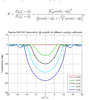
The reectivityR of the system shown in g. (2.6) is:

R = PB(ζ = 0)

PA(ζ = 0) =

kabsinh(−iq)

2

qcosh(−iq) + (

4β

2 )sinh(−iq)

[image:40.612.159.454.330.662.2]

2. (2.55)

(41)

[image:41.612.162.436.75.305.2]

Figure 2.6: Passive NIM-PIM DC reectivity at k =0, 2, 3, 4, & 5.

The above two gures, g. (2.5) and g. (2.6) show the three dierent regions that

have dierent values ofq , and how that aects the transmittivityT and reectivity

R of the structure. As long as

4β 2

>k, q becomes real, and the power exchange

takes the sinusoidal behavior. Once

4β 2

=k , q becomes 0, and neither output#1

nor output#2 has any power (i.e)T =R= 0. When

4β 2

<k q becomes imaginary,

and the power exchange takes the exponential behavior. The last case causes the re-ection of entire power back toward output#2. The colored codes above in g. (2.5)

and g. (2.6) show that clearly the transmittivity drops in the regions where

4β 2

(42)

2.4 Passive DFB Resonator

2.4.1 DFB Resonator

A distributed-feedback resonator consists of a periodic structure. Typically, the periodic structure is known as diraction grating. The structure is shown in g. (2.7). The exchange of power between the two output ports and the resulting power in output#1 and output#2 depend on some factors and one of them is the diraction grating.

Figure 2.7: DFB resonator

The coupled-mode equations for a passive DFB resonator can be written as [23]:

dA dζ =i

4β

2 A+ikbfB (2.56)

dB dζ =−i

4β

2 B−ikf bA, (2.57)

where A and B represent the forward and backward electromagnetic modes

(43)

backward wave and the coupling coecient of the backward wave into the forward

wave respectively, 4β represents the detuning between the waveguides.

4β =β1−β2, where β1 represents the propagation number of the light wave in

the waveguide, and β2 represents the propagation number of the grating structure,

and the mathematical form of the propagation number β2 in general is β2 = _Λπ ,

where Λ is the grating period.

The general solution can be written as:

A(ζ) = A1eiqζ +A2e−iqζ (2.58)

where q=ql, and it represents the normalized eigen-value

A quick look at equations (2.56), (2.57), (2.58), and (2.59) and comparing them respectively with equations (2.42), (2.43), (2.44), and (2.45), clearly shows that the passive NIM-PIM DC and the passive DFB resonator are governed by the same set

of coupled-mode equation and general solution. This means that all q , T , and R

will be the same which means that a passive NIM-PIM DC behaves like a passive DFB resonator

q=±

s

4β

2

−kf bkbf. (2.60)

T = PA(ζ = 1)

PA(ζ = 0)

= |q| 2

qcosh(−iq) +

4β

2 sinh(−iq)

(44)

R = PB(ζ = 0)

PA(ζ = 0) =

kabsinh(−iq)

2

qcosh(−iq) + (

4β

2 )sinh(−iq)

(45)

.

Chapter 3 3 Active NIM-PIM Directional Coupler

This chapter discusses the active structures like an active DFB resonator, and an active NIM-PIM DC. This discussion includes deriving and analyzing the structure's governing equations and their solutions. The equations are solved for the case of dierent coupling coecients for the rst time. The nal form of eigen-value, trans-mittivity, and reectivity for such structures were derived and analyzed. Also, the eect of coupling coecients for dierent scenarios were investigated and nal results were reported.

3.1 Active DFB Resonator

(46)

in chapter #2 where the time dependent phasor is e−iωt, normalize the equation

with the structure length l as ζ = z_l, and introduce a gain g in the structure. The

normalized coupled-mode equations of the DFB resonator can be written as follows [23]:

dA dζ =i(

4β

2 −i

g

2)A+ikbfB (3.1)

−dB

dζ =i(

4β

2 −i

g

2)B+ikf bA, (3.2)

where A(ζ) and B(ζ) represent the amplitude of electrical eld that travels

for-ward and backfor-ward respectively, kf b and kbf are the normalized forms of kf b and

kbf respectively, and kf b and kbf represent the coupling coecient of the

forward-propagation wave into the backward-forward-propagation wave and the coupling coecient of the backward-propagation wave into the forward-propagation wave in the DFB structure, respectively.

4β is the normalized form of 4β, and 4β = βa−βb represents the detuning

between the wavenumbers., where βb is the Bragg number, and it can be expressed

mathematically as β = _Λπ, where Λ represents the grating period. g =gl where g is

the normalized gain in the system.

The general solution of an active DFB resonator can be written as follows:

(47)

A1, A2, B1, and B2 are constant coecients.

d dζ A1e

=i(4β 2 −i

g

2) A1e

+ikbf B1eiqζ+B2e−iqζ

A1(iq)eiqζ+A2(−iq)e−iqζ =i( 4β

2 −i

g

2) A1e

+ikf b B1eiqζ +B2e−iqζ

.

A1(iq)eiqζ =i( 4β

2 −i

g

2) A1e iqζ

+ikbf B1eiqζ

(iq)A1 =i( 4β

2 −i

g

2)A1+ikbfB1

[q−(4β 2 −i

g

2)]A1 =kbfB1. (3.5)

Equating the terms that havee−iqζ _yields:

A2(−iq)e−iqζ =i( 4β

2 −i

g

2) A2e

−iqζ

+ikbf B2e−iqζ

(−iq)A2 =i( 4β

2 −i

g

(48)

[q+ (4β 2 −i

g

2)]A2 =−kbfB2. (3.6)

− d

dζ B1e

=i(4β 2 −i

g

2) B1e

iqζ₊_B 2e−iqζ

+ikf b A1eiqζ +A2e−iqζ

−B1(iq)eiqζ−B2(−iq)e−iqζ =i( 4β

2 −i

g

2) B1e iqζ

+B2e−iqζ

+ikf b A1eiqζ +A2e−iqζ

.

−B1(iq)eiqζ =i( 4β

2 −i

g

2) B1e iqζ

+ikf b A1eiqζ

−(iq)B1 =i( 4β

2 −i

g

2)B1+ikf bA1

[q+ (4β 2 −i

g

2)]B1 =−kf bA1. (3.7)

−B2(−iq)e−iqζ =i( 4β

2 −i

g

2) B2e

−iqζ

+ikf b A2e−iqζ

(iq)B2 =i( 4β

2 −i

g

(49)

[q−(4β 2 −i

g

2)]B2 =kbfA2. (3.8)

(3.8) into equation (3.6) gives us the value of the normalized eigen-valueq.

From equation (3.7), B1can be written as follows:

B1 =−

kf b

[q+ (4₂β −ig₂)]

A1.

SubstitutingB1value into equation (3.5) yields:

[q−(4β 2 −i

g

2)]A1 =kbf[−

kf b

{q+ (4₂β −ig₂)}]A1

[q−(4β 2 −i

g

2)][q+ ( 4β

2 −i

g

2)] =−kf bkbf

(q)2 = (4β 2 −i

g

2) 2₋_k

f bkbf

q=±

s

(4β 2 −i

g

2) 2₋_k

f bkbf. (3.9)

Equation (3.9) denes the normalized eigen-value q in terms of the normalized

wavenumber detuning 4β , the normalized gain g , and the normalized coupling

coecients kf b and kbf .

3.1.3 Amplier Boundary Conditions and Specic Solution

When the DFB resonator is used as a resonant type of amplier, no backward

(50)

equation (3.4) yields:

B(1) =B1eiq+B2e−iq

0 =B1eiq+B2e−iq

B2 =−B1ei2q. (3.10)

B(ζ) =B1eiqζ + (−B1ei2q)e−iqζ

B(ζ) = B1eiqζ −B1e(i2q−iqζ)

B(ζ) = B1(

e−iq

e−iq)(e

iqζ₋_e(i2q−iqζ)₎

B(ζ) = ( B1

e−iq)(e

i(qζ−q)₋

e−i(qζ−q)).

(51)

B(ζ) = 2B₁0sinh{i(qζ−q)}, (3.11)

where B₁0 = B1 e−iq

Substituting equation (3.11) into equation (3.2) gives us an expression for A(ζ)

as follows:

−dB

dζ =i(

4β

2 −i

g

2)B +ikf bA

− d

dζ[2B

0

1sinh{i(qζ −q)}] =i( 4β

2 −i

g

2)[2B

0

1sinh{i(qζ−q)}] +ikf bA

−2B₁0 d

dζ[sinh{i(qζ −q)}] =i(

4β

2 −i

g

2)[2B

0

−2B₁0(iq)cosh{i(qζ−q)}=i(4β 2 −i

g

2)[2B

0

−2B₁0(q)cosh{i(qζ−q)}= (4β 2 −i

g

2)[2B

0

1sinh{i(qζ−q)}] +kf bA

kf bA=−2B10(q)cosh{i(qζ −q)} −( 4β

2 −i

g

2)[2B

0

1sinh{i(qζ −q)}]

kf bA=−2B10[(q)cosh{i(qζ −q)}+ ( 4β

2 −i

g

2)(sinh{i(qζ−q)})]

A(ζ) = −2B

0

1

kf b

qcosh{i(qζ −q)}+ (4β 2 −i

g

2)sinh{i(qζ−q)}

(52)

Now, using the well known relationship between the power P and the amplitude

A, P = |A|2, we can easily nd the power in each light direction and calculate the

transmittivity and reectivity of the system as follows:

PA=|A(ζ)| 2 =

−2B₁0 kf b

[qcosh{i(qζ−q)}+ (4β 2 −i

g

2)sinh{i(qζ −q)}]

2

PB =|B(ζ)|2 =|2B10sinh{i(qζ−q)}| 2

,

where PA and PB are the power in forward and backward directions respectively.

The transmitivity T of the system (output #1, Fig. (3.1 )is:

T = PA(ζ = 1)

PA(ζ = 0)

= |q| 2

qcosh(−iq) + (

4β 2 −i

g

2)sinh(−iq)

2. (3.13)

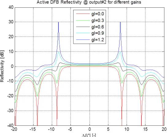
The reectivityR of the system (output #2, Fig. (3.2 )is:

R = PB(ζ = 0)

PA(ζ = 0) =

k_{f b}sinh(−iq)

2

qcosh(−iq) + (

4β 2 −i

g

2)sinh(−iq)

(53)

[image:53.612.163.434.75.303.2]

Figure 3.1: Active DFB resonator transmittivity at k = 3.

Figure 3.2: Active DFB resonator reectivity at k = 3.

The above two gures, g. (3.1) and g. (3.2) depict the behavior of transmittivity and reectivity of an active DFB resonator respectively. Clearly seen is that at

[image:53.612.163.437.364.587.2]

(54)

the two structure's outputs (output #1and output #2) can emit power that reaches innity and introduces lasing behavior.

3.2 Active NIM-PIM DC

We stick with the same convention of electromagnetic eld denition that we used in

chapter #2 where the time dependent phasor is e−iωt , normalize the equation with

the structure lengthl asζ = z_l,and introduce gains gp and gn in the PIM waveguide

and NIM waveguide respectively. The normalized coupled mode equations of an active NIM-PIM-DC can be written as follows [11]:

dA dζ =i(

4β

2 −i

gp

2)A+ikbaB (3.15)

−dB

dζ =i(

4β

2 −i

gn

2)B+ikabA, (3.16)

whereA(ζ) and B(ζ) represent the amplitude of electrical eld that travels forward

and backward respectively, kab and kba are normalized form of coupling coecients

kab and kba, respectively, and kab and kba represent the coupling coecient of the

waveguide A into the waveguide B and the coupling coecient of the waveguide B into the waveguide A, respectively

4β is the normalized form of 4β, and 4β = βa−βb represents the detuning

between the wavenumbers, where βa and βb represent the wavenumber in PIM and

NIM waveguides respectively. β = 2_λπ

on, where n represents the modal refractive

index, and λo represents the wavelength in the air. gp and gn are normalized form

(55)

PIM waveguide and in NIM waveguide, respectively.

The general solution of an active NIM-PIM DC can be written as follows:

B(ζ) = B1eiq

0_ζ

+B2e−iq

0_ζ

, (3.18)

whereqandq0 are the normalized form of_qand_q0_{, respectively, and}_q_and_q0 _represent

the eigen-value of the PIM and NIM waveguides, respectively. The mathematical form that relates the two eigen-value can be written as follows:

q0 ₌_q₊_x, (3.19)

where x is the value that will be derived in this chapter and will give us the nal

solution for the transmittivity T and the reectivity R for this kind of structures

and A1, A2, B1, and B2 are constant coecients.

3.2.2 Dispersion Relation and Eignvalue

d dζ A1e

iqζ₊_A 2e−iqζ

=i(4β 2 −i

gp 2) A1e

iqζ₊_A 2e−iqζ

+ikba

B1eiq

0_ζ

+B2e−iq

0_ζ

A1(iq)eiqζ+A2(−iq)e−iqζ =i( 4β

2 −i

gp 2) A1e

iqζ

+A2e−iqζ

+ikba

B1eiq

0_ζ

+B2e−iq

0_ζ

(56)

A1(iq)eiqζ =i( 4β

2 −i

gp 2) A1e

iqζ

(iq)A1 =i( 4β

2 −i

gp

2)A1. (3.20)

A2(−iq)e−iqζ =i( 4β

2 −i

gp 2) A2e

−iqζ

(−iq)A2 =i( 4β

2 −i

gp

2)A2. (3.21)

Equating the terms that haveeiq0ζ yields:

0 = ikba(B1eiq

0_ζ

)

0 =ikbaB1. (3.22)

Equating the terms that havee−iq0ζ yields:

0 =ikba(B2e−iq

0_ζ

)

0 =ikbaB2. (3.23)

(57)

− d

dζ

B1eiq

0_ζ

+B2e−iq

0_ζ

=i(4β 2 −i

gn 2 )

B1eiq

0_ζ

+B2e−iq

0_ζ

+ikab A1eiqζ +A2e−iqζ

−B1(iq0)eiq

0_ζ

−B2(−iq0)e−iq

0_ζ

=i(4β 2 −i

gn 2 )

B1eiq

0_ζ

+B2e−iq

0_ζ

+ikab A1eiqζ +A2e−iqζ

.

Equating the terms that haveeiqζ _yields:

0 =ikab(A1eiqζ)

0 =ikabA1. (3.24)

Equating the terms that haveeiqζ _yields:

0 =ikab(A2e−iqζ)

0 =ikabA2. (3.25)

Equating the terms that haveeiq0ζ yields:

−B1(iq0)eiq

0_ζ

=i(4β 2 −i

gn 2)

B1eiq

0_ζ

(−iq0₎_B

1 =i( 4β

2 −i

gn

2 )B1. (3.26)

Equating the terms that havee−iq0_ζ

(58)

−B2(−iq0)e−iq

0_ζ

=i(4β 2 −i

gn 2 )

B2e−iq

0_ζ

(iq0₎_B

2 =i( 4β

2 −i

gn

2 )B2. (3.27)

Now, combining both equations (3.20) and (3.22) yields:

(iq)A1 =i( 4β

2 −i

gp

2)A1+ikbaB1

qA1 = ( 4β

2 −i

gp

2)A1+kbaB1

(q−4β 2 +i

gp

2)A1 =kbaB1. (3.28)

Combining both equations (3.21) and (3.23) yields:

(−iq)A2 =i( 4β

2 −i

gp

2)A2+ikbaB2

−qA2 = ( 4β

2 −i

gp

2)A2+kbaB2

(q+4β 2 −i

gp

2)A2 =−kbaB2. (3.29)

(−iq0₎_B

1 =i( 4β

2 −i

gn

(59)

−q0_B

1 = ( 4β

2 −i

gn

2)B1+kabA1

(q0₊ 4β

2 −i

gn

2 )B1 =−kabA1. (3.30)

(iq0₎_B

2 =i( 4β

2 −i

gn

2 )B2+ikabA2

q0_B

2 = ( 4β

2 −i

gn

2)B2+kabA2

(q0₋ 4β

2 +i

gn

2 )B2 =kabA2. (3.31)

Now, we left o with four equations (3.28), (3.29), (3.30), and (3.31) with four constants A1,B1, A2,and B2.

Now, substituting equation (3.30) into equation (3.28) yields the following:

From equation (3.30) we have:

(q0 ₊4β

2 −i

gn

2 )B1 =−kabA1

B1 =−

kab

(q0 ₊4β 2 −i

gn

2 )

A1.

Applying this value ofB1into equation (3.28) yields:

(q− 4β 2 +i

gp

2)A1 =kba −

kab

(q0 ₊4β 2 −i

gn

2 )

!

(60)

(q−4β 2 +i

gp 2)(q

0₊4β

2 −i

gn

2) = −kabkba.

Taking the product of the left hand side yields:

qq0₊_q₍4β

2 )−iq(

gn 2 )−q

0₍4β

2 )−( 4β

2 )

2₊_i₍4β 2 )(

gn 2)+iq

0₍gp

2)+i( 4β 2 )( gp 2)+( gp 2)( gn

2) = −kabkba

qq0₊_q₍4β

2 −i

gn 2 )−q

0₍4β

2 −i

gp 2) + (

4β

2 )(i

gp 2 +i

gn 2)−(

4β2

4 ) + (

gpgn

4 ) =−kabkba.

(3.32)

Now, substituting equation (3.31) into equation (3.29) yields the following:

From equation (3.31) we have:

(q0 ₋4β

2 +i

gn

2 )B2 =kabA2

B2 =

kab

(q0 ₋4β 2 +i

gn

2 )

A2.

Applying this value ofB2into equation (3.29) yields:

(q+ 4β 2 −i

gp

2)A2 =−kba

kab

(q0 ₋4β 2 +i

gn

2 )

!

A2

(q+4β 2 −i

gp 2)(q

0₋ 4β

2 +i

gn

2) = −kabkba.

(61)

qq0₋_q₍4β

2 )+iq(

gn 2 )+q

0₍4β

2 )−( 4β

2 )

2₊_i₍4β 2 )(

gn 2 )−iq

0₍gp

2)+i( 4β 2 )( gp 2)+( gp 2)( gn

2) = −kabkba

qq0₋_q₍4β

2 −i

gn 2 ) +q

0₍4β

2 −i

gp 2) + (

4β

2 )(i

gp 2 +i

gn 2)−(

4β2

4 ) + (

gpgn

4 ) =−kabkba.

(3.33)

Adding both equations (2.32) and (2.33) yields:

2(qq0_{) + 2(}4β

2 )(i

gp 2 +i

gn 2 )−2(

4β

2 )

2_{+ 2(}gpgn

4 ) + 2(kabkba) = 0.

Dividing the above equation by 2 yields:

(qq0_{) + (}4β

2 )(i

gp 2 +i

gn 2 )−(

4β

2 )

2_{+ (}gpgn

4 ) + (kabkba) = 0.

Rearranging the above equation yields:

qq0₋_[(4β

2 ) 2₋

(kabkba)−( 4β

2 )(i

gp 2 +i

gn 2 )−(

gpgn

4 )] = 0. (3.34)

Subtracting equations (2.33) from equation (2.32) yields:

2q(4β 2 −i

gn 2 )−2q

0₍4β

2 −i

gp 2) = 0.

Dividing the above equation by 2 yields:

q(4β 2 −i

gn 2)−q

0₍4β

2 −i

(62)

q(4β 2 −i

gn 2 ) = q

0₍4β

2 −i

gp 2).

Substituting equation (3.19) in the above equation yields:

(q0₋_x₎₍4β

2 −i

gn 2) = q

0₍4β

2 −i

gp 2)

q0₍4β

2 )−q

0₍_ign

2)−x( 4β

2 ) +x(i

gn 2 ) = q

0₍4β

2 )−q

0₍_igp

2).

Rearranging the above equation yields:

−q0₍_ign

2 ) +q

0₍_igp

2) =x( 4β

2 )−x(i

gn 2)

q0₍_igp

2 −i

gn 2 ) =x(

4β

2 −i

gn 2 )

x=q0(i

gp

2 −i gn

2 ) (4₂β −ign

2 )

. (3.35)

Let us introduce another quantity calledH, and let it has the following relationship

with x:

H = x

q0 (3.36)

H = (i gp

2 −i gn

2 ) (4₂β −ign

2 )

. (3.37)

Now, the relationship between both normalized eign-values q and q0 using the new

(63)

q =q0₋_x

q=q0₋_q0_H

q=q0₍₁₋_H₎_. (3.38)

qq0₋_[(4β

2 ) 2₋

(kabkba)−( 4β

2 )(i

gp 2 +i

gn 2)−(

gpgn 4 )] = 0

[q0₍₁₋_H_)]_q0 ₋_[(4β

2 ) 2 ₋₍_k

abkba)−( 4β

2 )(i

gp 2 +i

gn 2)−(

gpgn 4 )] = 0

(q0₎2₍₁₋_H₎₋_[(4β 2 )

2₋₍_k

abkba)−( 4β

2 )(i

gp 2 +i

gn 2 )−(

gpgn

4 )] = 0.

Using the quadratic formulax= −b±

√ (b2₋₄_ac₎

2a yields:

q0 ₌_±

s

(4(1−H)[(

4β

2 )2−(kabkba)−(

4β 2 )(i

gp

2 +i gn

2 )−( gpgn

4 )] 4(1−H)2 )

q0 ₌_±

s

((

4β 2 )

2₋₍_k

abkba)−(4₂β)(ig₂p +ig₂n)−(gp₄gn)

(1−H) ). (3.39)

3.2.3 Amplier Boundary Conditions and Specic Solution

When the NIM-PIM DC is used as a type of amplier, no backward propagating

(64)

(3.18) yields:

B(ζ) =B1eiq

0_ζ

+B2e−iq

0_ζ

B(1) =B1eiq

0

+B2e−iq

0

0 =B1eiq

0

+B2e−iq

0

B2 =−B1ei2q

0

. (3.40)

B(ζ) =B1eiq

0_ζ

+B2e−iq

0_ζ

B(ζ) =B1eiq

0_ζ

+ (−B1ei2q

0

)e−iq0ζ

B(ζ) =B1eiq

0_ζ

−B1e(i2q

0₋_iq0_ζ₎

B(ζ) = B1(

e−iq0

e−iq0)(e

iq0_ζ

−e(i2q0−iq0ζ))

B(ζ) = ( B1

e−iq0)(e

i(q0_ζ₋_q0₎

−e−i(q0ζ−q0)).

(65)

B(ζ) = 2B₁0sinh{i(q0_ζ₋_q0_)}_, (3.41)

where B₁0 = B1

e−iq0

Substituting equation (3.41) into equation (3.16) gives us an expression forA(ζ)

as follows:

−dB

dζ =i(

4β

2 −i

gn

2 )B+ikabA

− d

dζ[2B

0

1sinh{i(q0ζ−q0)}] =i( 4β

2 −i

gn 2)[2B

0

1sinh{i(q0ζ−q0)}] +ikabA

−2B₁0 d

dζ[sinh{i(q

0_ζ₋_q0_{)}] =}_i₍4β

2 −i

gn 2)[2B

0

−2B₁0(iq0₎_cosh_{_i₍_q0_ζ₋_q0_)}₌_i₍4β

2 −i

gn 2)[2B

0

−2B₁0(q0₎_cosh_{_i₍_q0_ζ₋_q0_)}_{= (}4β

2 −i

gn 2)[2B

0

1sinh{i(q0ζ−q0)}] +kabA

kabA=−2B10(q0)cosh{i(q0ζ−q0)} −( 4β

2 −i

gn 2)[2B

0

1sinh{i(q0ζ−q0)}]

kabA =−2B10[(q0)cosh{i(q0ζ−q0)}+ ( 4β

2 −i

gn

2 )(sinh{i(q

0_ζ₋_q0_)})]

A(ζ) = −2B

0

1

kab

q0_cosh_{_i₍_q0_ζ₋_q0_)}_{+ (}4β

2 −i

gn

2)sinh{i(q

0_ζ₋_q0_)}

(66)

Using the well known relationship between the power P and the amplitude A,

P = |A|2, we can easily nd the power in each light direction and calculate the

transmittivity and reectivity of the system as follows:

PA=|A(ζ)|2 =

−2B₁0 kab

[q0_cosh_{_i₍_q0_ζ₋_q0_)}_{+ (}4β

2 −i

gn

2 )sinh{i(q

0_ζ₋_q0_)}]

2

PB =|B(ζ)|2 =

2B

0

1sinh{i(q0ζ−q0)}

2

,

where PA and PB are the power in forward and backward directions respectively.

The transmitivity T of the system (output #1, Fig. (2.4 )is:

T = PA(ζ = 1)

PA(ζ = 0) = q0 2 q

0_cosh₍₋_iq0_{) + (}4β 2 −i

gn

2 )sinh(−iq

0₎

2. (3.43)

The reectivityR of the system (output #2, Fig. (2.4 )is:

R = PB(ζ = 0)

PA(ζ = 0) =

k_absinh(−iq0) 2 q

0_cosh₍₋_iq0_{) + (}4β 2 −i

gn

2 )sinh(−iq

0₎

2. (3.44)

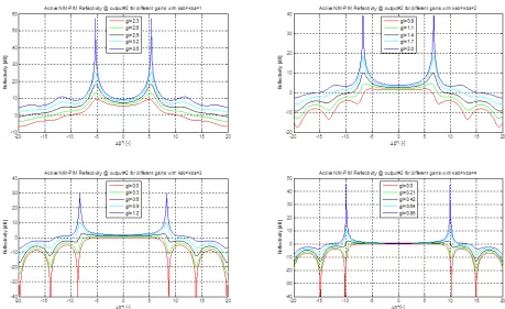
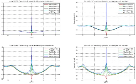
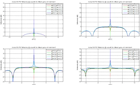
The above two expressions for transmittivityT and reectivityRare general enough

to consider any value of gp, gn, kab, kba, ∆β, and q0. Some specic scenarios2 are

discussed here, and they are divided to lasing and non-lasing scenarios. Some lasing scenarios are:

2_{The eigen-value} _q0 _{, transmittivity}_T _{, and reectivity} _R _{for each scenario are derived in the}

(67)

[image:67.612.109.567.101.391.2]

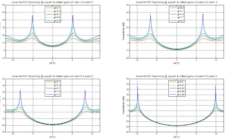
Scenario #1: gp =gn=g and 4k= 0.

(68)

[image:68.612.101.560.73.354.2]

(69)

[image:69.612.107.566.104.389.2]

Scenario #2: gp =gn=g and 4k6= 0.

(70)

[image:70.612.101.557.73.354.2]

(71)

(72)

(73)

Scenario #3: gp =g, gn = 0, and 4k = 0.

Figure 3.9: Scenario #3 transmittivity.

(74)

Scenario #4: gp =g, gn = 0, and 4k 6= 0.

(75)

(76)

[image:76.612.109.572.105.392.2]

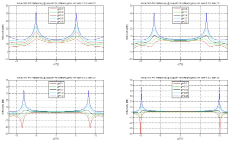
Scenario #5: gp =g, gn =−g, and4k = 0.

(77)

[image:77.612.103.569.73.356.2]

(78)

[image:78.612.107.567.99.392.2]

Scenario #6: gp =g, gn =−g, and4k 6= 0.

(79)

[image:79.612.107.568.72.359.2]

(80)

(81)

Figure 3.18: Scenario #6 reectivity contineous.

• Some non-lasing scenarios are:

Scenario #1: gp =any, gn =any, and (kab and/orkba) = 0.

(82)

3.2.5 Lasing and non-Lasing Combinations

From the previous dierent scenarios of an active NIM-PIM DC, the following table of multimode and single mode lasing and non-lasing combinations can be concluded:

Table (3.1) Active NIM-PIM DC Lasing Combinations

Conguration Parameters Lasing Behavior

gp gn 4k =kab−kba # Lasing Modes Lasing Threshold

any any kab and/orkba= 0 No lasing

> 0 gp = 0 Multi-mode Lowergthwith biggerk

> 0 gp 6= 0 Multi-mode Higher gthwith bigger 4k

> 0 0 = 0 Multi-mode Lowergthwith biggerk

> 0 0 6= 0 Multi-mode Higher gthwith bigger 4k

> 0 0 kab and/or kba ≤2.5 No lasing

> 0 < 0 = 0 Single-mode Higher gthwith bigger k

(83)

.

Chapter 4 4 Lasing Behavior

4.1 Lasing Action

The laser (Light Amplication by Stimulated Emission of Radiation) happens when spontaneous emission occurs inside a gain medium and conned by mirrors. Once these spontaneous photons go back and forth through this gain medium, an other emission happens. The later emission called stimulated emission; This emission and the movement of the new generated photons inside the gain medium will amplify the light by increasing the number of light photons.

(84)

the gain pass the loss is called threshold condition; the conditions that are needed to produce a laser are called lasing conditions [22]. These conditions include gain, wavenumber detuning, coupling coecients, and several others, and they change from one medium to another.

Laser Modes can be single-mode or multi-mode. Also, the traveling wave in a medium like our case above consists of longitudinal and transverse modes. All these denition are well known and repeatedly discussed everywhere, so I am just mentioned them without details. One thing important I have to mention here is the term of single-mode operation. In chapter 3 of this thesis we reported a single mode lasing using an active NIM-PIM DC with dierent coupling coecients. The single mode lasing can be divided into two main categories which are:

• single-transverse mode.

• single-longitudinal mode.

Our single-mode lasers have a single transverse and longitudinal mode.