City, University of London Institutional Repository
Citation
:
Kharchenko, V. S., Odarushchenko, O., Odarushchenko, V. and Popov, P. T. (2013). Selecting Mathematical Software for Dependability Assessment of Computer Systems Described by Stiff Markov Chains. Paper presented at the 9th International Conference on ICT in Education, Research and Industrial Applications: Integration, Harmonization and Knowledge Transfer, 19-06-2013 - 22-06-2013, Kherson, Ukraine.This is the accepted version of the paper.
This version of the publication may differ from the final published
version.
Permanent repository link: http://openaccess.city.ac.uk/4362/
Link to published version
:
Copyright and reuse:
City Research Online aims to make research
outputs of City, University of London available to a wider audience.
Copyright and Moral Rights remain with the author(s) and/or copyright
holders. URLs from City Research Online may be freely distributed and
linked to.
City Research Online: http://openaccess.city.ac.uk/ [email protected]
Selecting mathematical software for dependability
assessment of computer systems described by stiff
Markov chains
Vyacheslav Kharchenko1,2,*, Oleg Odarushchenko2, Valentina Odarushchenko1,
and Peter Popov3
1 National Aerospace University “KhAI”, Kharkov, Ukraine {v.kharchenko, v.odarushchenko}@khai.edu
2 RPC “Radiy”, Kirovograd, Ukraine
3 Centre for Software Reliability, City University London, United Kingdom
Abstract. Markov and semi-Markov models are widely used in dependability assessment of complex computer-based systems. Model stiffness poses a serious problem both in terms of computational difficulties and in terms of accuracy of the assessment. Selecting an appropriate method and software package for solving stiff Markov models proved to be a non-trivial task.
In this paper we provide an empirical comparison of two approaches to dealing with stiffness – stiffness avoidance and stiffness-tolerance. The study includes several well known techniques and software tools used for solving Kolmogorov’s differential equations derived from complex stiff Markov models.
In the comparison we used realistic cases studies developed by others in the past: i) a computer system with hardware redundancy and diverse software, and ii) a queuing system with a server break-down and repair. The results indicate that the accuracy of the known methods is significantly affected by the stiffness of the Markov models, which led us to developing a procedure (an algorithm) for selecting the optimal method and tool for solving a given stiff Markov model. The algorithm is, also included in the paper.
Keywords. Markov chins, stiffness, stiffness-avoidance, stiffness-tolerance, computer based systems, availability, multi-fragmentation.
Key Terms. Markov chains, stiffness, availability, multi-fragmentation
1
Introduction
handle well complex situations such as failure/repair dependencies and shared repair resources [3].
Dependability assessment of complex computer systems is an essential part of the development process as it either allows for demonstrating that relevant regulations have been met (e.g. as in safety critical applications) and/or for making informed decisions about the risks due to automation (e.g. in applications when poor dependability may lead to huge financial losses). Achieving these goals, however, requires accurate assessment. Assessment errors may lead to wrong or suboptimal decisions.
System modellers are often interested in transient measures, which provide more
useful information than steady-state measures. The main computational difficulty when MC are used is the size of the models (i.e. their largeness), which is known to affect the accuracy of the transient numerical analysis.
It is not unusual for modern complex systems to have a very large state space: often it may consist of tens of thousands of states. Additional difficulty in solving such
models is the model stiffness [5], which is the focus of this paper. In practice stiffness
in models of computer systems is caused by: i) in case of repairable systems the rates of failure and repair differ by several orders of magnitude [4]; ii) fault-tolerant computer systems (CS) use redundancy. The rates of simultaneous failure of redundant components are typically significantly lower than the rates of the individual components [4]; iii) in models of reliability of modular software the modules’ failure rates are significantly lower than the rates of passing the control from a module to a module [4].
In practice it is useful to detect the model stiffness as early as possible. If the model is stiff, using a small integration step is usually a necessary step for obtaining an accurate solution. On the other hand, models with moderate stiffness may allow for obtaining accurate solutions without using a small integration step, thus saving computational resources. With some numerical methods decreasing the step of integration mat be even counterproductive as it may simply not improve the solution accuracy.
The assessment methods and tools must provide high confidence in the assessment results. In many cases various regulation bodies would require the tools used in the development to be certified to meet stringent quality requirements. The stiffness of an MC can make it difficult to meet this requirement. Careful selection of the method and tools used to solve accurately and efficiently stiff MCs is needed.
In the last 30 years, many approaches have been developed to deal efficiently with the MC stiffness [4, 5, 6, 7]. They can be split into two groups - “stiffness-tolerance” (STA) and “stiffness-avoidance” approaches (SAA) [5]. The main feature of STA is
solving a stiff MC using special numerical methods that can provide highly accurate
results. The limitations of STA are: i) STA cannot deal effectively with large models, and ii) computational efficiency is difficult to achieve when highly accurate solutions
are sought. The SAA solution, on the other hand, is based on an approximation
algorithm which converts a stiff MC to a non-stiff chain first, which typically has a significantly smaller state space [4]. An advantage of this approach is that it can deal effectively with large stiff MCs. Achieving high accuracy with SAA, however, may be problematic.
is the utility developed by some of the authors of this paper (ODU) developed more than 15 years ago which is based on EXPMETH [21] and has been validated extensively
on a range of models [18 - 20]. The utility uses the algorithm of modified exponential
method. In addition, a number of off-the-shelf mathematical software packages exist which can be used for solving Markov models, e.g. Maple (Maplesoft), Mathematica (Wolfram Research) and MATLAB (Mathworks) which use standard methods for solving differential equations. These math packages enjoy high reputation among the respective customers earned over several decades by providing a wide range of solutions and good support with regular updates.
In this paper we present an empirical study using two systems: i) a computer system with hardware redundancy and diverse software under the assumptions that the rate of failure of software may vary over time, and ii) a queuing system with a server break-down and repair [4]. The solution of the first system is based on the principle of multi-fragmentation [9], one of the efficient methods of solving an MC in case the model parameters change over time. The main idea of this principle is that the MC is
represented as a set of fragments with identical structure, but which differ in the values
of one or more parameters. Each of the systems included in the study is described by a stiff MC. The main difference between the two systems is that the ratio between the
stiffness indices (to be defined below) of the first and the second system is 103. In other
words we chose them to be quite different in terms of their stiffness index so that we could study if the stiffness index impacts the accuracy of the different methods for solving the respective models. Both systems were solved using STA. The second system was also solved using SAA. Thus we could compare the accuracy of STA and SAA when applied to solving the same (the second) system and how these compare with the exact solution, which for the second system is available in [10], [11].
We report that indeed the stiffness index impacts significantly the accuracy of the solution methods. We also offer a selection procedure which allows one to choose (among the many available for solving stiff MCs) the solution method that provides the best accuracy given the value of the stiffness index of the MC to be solved. We provide also a justification for our recommendations based on the comparison of the different methods when applied to the chosen two systems described by stiff MCs.
The numerical transient analysis of MCs is faced with two computational difficulties – the model stiffness and largeness, which can affect the accuracy of the solutions obtained. Several numerical methods are widely used that address these difficulties, among them the Rosenbrock method [13], [14], the TR-BDF2 [5], [7], [14], the Jensen’s method (uniformization) [5], the implicit Runge-Kutta method [5], [6], [12], and the modified Gir method [6].
The Rosenbrock method is the one-step numerical method that has the advantage of being relatively simple to understand and implement. For moderate accuracy (tolerances of order 10-4 – 10-5) and systems of moderate-size (N ≲ 10) the method
allows for obtaining solutions which in terms of achieved accuracy are comparable with the more complex algorithms. If a low accuracy is acceptable, then this method is attractive. When larger systems are solved the Rosenbrock method becomes less accurate and reliable [13].
increased stiffness and only requires little extra computations as the parameter values or the mission time are increased. TR-BDF2 is also recommended for use if low accuracy is acceptable [5].
The Jensen method (also known as uniformization or randomization) [15] involves
the computation of Poisson probabilities. It was extensively modified [5], [14], [16] to deal with the stiffness problem. It achieves greater accuracy than TR-BDF2 but still deals poorly with stiffness in extreme cases. [14] recommends that the Jensen method be used only in cases of moderately stiff models.
The implicit Runge-Kutta method is a single step numerical method that deals with the problem of stiffness and is one of the most computationally efficient methods for achieving high accuracy [6].
Also an aggregation/disaggregation technique for transient solution of stiff MCs was developed by K. S. Trivedi and A. Bobbio [4]. The technique can be applied to any
MC, for which the transition rates can be grouped into two separated sets of values: one
of the sets would include the “slow” states and the second set would include the “fast” states [4]. After aggregating the fast transition rates the MC is reduced to a smaller non stiff MC, which can be solved efficiently using a standard numerical technique [4].
In the rest of the paper the method by Trivedi and Bobbio [4] is referred to as an SAA while the other methods surveyed above are referred to as an STA.
The focus of this study is a comparison of the accuracy of the solution obtained with different methods when applied to the same system. Of particular interest is how the solutions are affected by the stiffness of the system under study.
The rest of the paper is organized as follow: in the section 2 we describe formally the stiffness problem and the stiffness index introducing informally the idea of how stiffness index may impact the accuracy of the numerical methods used in solving the systems. In section 3 we present the comparison results. In section 4 we present a procedure for selecting the optimal solution method and tool based on the stiffness index of an MC. In section 5 we present the conclusions and the problems left for future research.
2
Comparative Analysis of Evaluation Techniques
2.1 The Stiffness Problem
Stiffness is an undesirable property of many practical MCs that pose difficulties in finding transient solutions. There is no commonly adopted definition of “stiffness” but a few of the most widely used ones are summarized below.
a) The Cauchy problem 𝑑𝑢𝑑𝑥= 𝐹(𝑥, 𝑢) is said to be stiff on the interval [x0,X] if for
x from this interval the following condition is fulfilled:
1 | ) Re( | min
| ) Re( | max ) (
, 1 ,
1
i n i
i n i
x s
, (1)
where the s(x) – denotes the index of stiffness (stiffness index) and λi – are the
Also the index of stiffness of an MC was defined in [5], [14] as the product of the largest total exit rate from a state and the length of solution interval(=λit), where λi are
the eigenvalues of the Jacobian matrix.
b) A system of differential equations (DE) is said to be stiff on the interval [0,t) if
there exists a solution component of the system that has variation on that interval that
is large compared to 1/t. Thus, the length of the solution interval also becomes a
measure of stiffness [14], [17].
We use the index of stiffness in the empirical evaluations that follow as a measure of discrimination between the MCs with different indices of stiffness: high-stiffness (s(x) ≥103), moderate-stiffness (102< s(x) <103) and low-stiffness (s(x) ≤ 102).
Here we provide an illustration of how the index of stiffness can affect the accuracy achievable by numerical methods of solving a system of the DEs, which describes a stiff MC.
The most common type of a stiff linear system of DEs is the system in which the eigenvalues can be divided into two groups, based on the difference in their modulus values. The eigenvalues of the first group with large modulus values determine the solution behaviour in the boundary layer. Their corresponding components are rapidly decreasing. The eigenvalues of the second group with small modulus values determine the solution behaviour out of the boundary layer. The index of stiffness (1) is the ratio between the maximum value from the first group and the minimum value from the second one.
To describe in detail the influence of this separation on the stability of the numerical methods let us consider a DE matrix with constant coefficients,
M
j
i
a
A
Ay
y
,
(
ij),
,
1
,...,
(2)
M
i
y
y
y
y
(
0
)
0,
i
(
0i),
1
,...,
(3)
Matrix A is a simple-structured matrix, which means that it has M linearly
independent eigenvectors and 𝜆𝑖, 𝑒𝑖 – are the eigenvalues and the corresponding
eigenvectors of matrix A, respectively. The solution of the Cauchy problem (2) with initial conditions (3) is presented in (4):
Mi
i x i
e
e
C
x
y
i1
)
(
(4)
Each component 𝐶𝑖𝑒𝜆𝑖𝑥𝑒𝑖 present in the solution (4) is proportional to one of the
eigenvectors and is integrated independently of the other components.
If matrix А has large absolute negative eigenvalues a very small step h would be required on the whole integration interval. With a large integration interval this limitation would cause an increase of the local round-off errors, which would become a serious problem if high overall accuracy is sought.
As an example let’s consider a system of two differential equations. Without loss of generality let us assume that |𝜆1| ≫ |𝜆2|.
The exact solution (4) will take the following form:
y
(
x
)
C
1e
1xe
1
C
2e
2xe
2The first component of of the solution will decrease rapidly on the interval∽ 𝜏 =
1/|𝜆1|, and after that will become extremely small. In this interval this component
influences the solution y(x). The second component changes on the interval 𝜏 ∽ 1/|𝜆2|.
The second interval is much wider than the first one. In this interval the second
component influences the solution y(x). In the first interval the rate of solution change
is high and it is dominated by the change of the first component. In the second interval, the rate of change is small and is dominated by the change of the second component. As we can see the values of the given coefficients affect the behaviour of the transient solution. On the first interval, the so called boundary layer, in order to achieve an accurate solution in the presence of rapid changes, the step-size must satisfy the
condition ℎ ≪ 1/|𝜆1|. In the second interval the same condition on the step is required,
because the corresponding component of the DE must decrease.
[image:7.595.132.465.380.505.2]The example despite its simplicity provides a clear illustration of how different eigenvalues may lead to the need for changing the step-size in different integration intervals so that accurate results may be obtained. The value of the stiffness index (1) clearly affects the accuracy achievable with a given solution method. The higher the stiffness index the stricter the requirements imposed on the stability of the chosen numerical method.
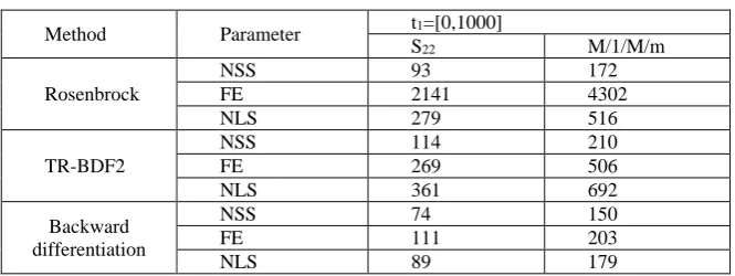
Table 1. Experiment results
Method Parameter t1=[0,1000]
S22 M/1/M/m
Rosenbrock
NSS 93 172
FE 2141 4302
NLS 279 516
TR-BDF2
NSS 114 210
FE 269 506
NLS 361 692
Backward differentiation
NSS 74 150
FE 111 203
NLS 89 179
We study in detail the impact of the stiffness index on the achievable accuracy with different numerical methods using two stiff MCs with substantially different stiffness indices, s(x). The first stiff MC is a model of a computer system with hardware
redundancy and diverse software (S22) [21]. The second system is a queuing system
with server break-down and repair (M/M/1/k) [5]. The first system is of
moderate-stiffness, with s(x)=4*102(1), where max |Re(λ
i)| = 0.2 and min|Re(λi)| = 0.0005. The
MC of the second system is of high-stiffness, with s(x) = 3.0001*104, where max
|Re(λi)|= 3.0001 and min|Re(λi)|=0.0001. Both MCs are of equal size – 20 states. The
study was conducted using the functions for solving stiff DEs implemented in the
mathematical package MATLAB – ode23s, ode23tb, ode15s, whichimplement the
Rosenbrock method, the TR-BDF2 and the method of backward differentiation, respectively.
Table 1 summarizes the parameters obtained with the different methods for solving stiff DE: the number of successful steps (NSS), the function evaluations (FE) and the
Table shows that even when the model largeness is the same the solution for a system of high-stiffness, M/1/M/m, requires nearly twice as many steps, function evaluations and linear system solutions.
2.2 Stiffness-tolerance and Stiffness-avoidance Approaches
Stiffness-tolerance approach. The main idea of this approach is using methods that are stable for solving stiff models. These can be split into two broadly classes: “classical” numerical methods for solution of stiff DEs and “modified” numerical methods used for finding a solution in special cases.
a) The classical (non-modified) numerical methods for solving stiff DEs use special
single-step and multi-step integration methods. Examples of such methods are the implicit Runge-Kutta, the TR-BDF2, the Rosenbrock method, the exponential method, the implicit Gir method described in [5], [6], [7], [13], respectively. The implicit Runge-Kutta, TR-BDF2 and Rosenbrock method are implemented by several mathematical off-the-shelf software packages and are usually considered the most accurate methods for solving stiff ODEs.
b) An example of the modified numerical methods is the exponential modified
method. The original algorithm was presented in [6] and is based on the evaluation of the matrix exponent. In [6] this method is recommended as one of the most effective algorithms for solving the class of ODE systems with a high value of the Lipchitz constant, and as a special part of a stiff ODE. As a modification part, an automated adaptive step of integration can be implemented [6]. As the method has a multi-step algorithm the given modification can increase the accuracy of the solution. The amount of computations and the machine time needed for the solution of stiff DEs can be reduced, too, [6].
The solution provided by using any numerical method is expected to be accurate. However, typically the result obtained with numerical method include errors coming
from different sources, such as: problem statement error - an inherent error, due to
various simplifications introduced in order to make the problem (analytically) tractable; truncation error -the error related to truncating the infinite series after a finite number
of terms are computed; round-off error - the type of error that arises in every arithmetic
operation carried out on a computer; initial error - the error related to the presence of
approximate parameters in the mathematical formulae. Ideally we would like to control each of these components of the computational error.
Stiffness-avoidance approach. The basic idea of this approach is a model transformation by identifying and eliminating the stiffness from the model, which would bring two benefits: i) a reduction of the largeness of the initial MC, and ii) efficiency in solving a non-stiff model using standard numerical methods. The approach was named an aggregation/disaggregation technique for transient solution of stiff MCs. The technique, developed by K. S. Trivedi, A. Bobbio and A. Reibmann [4], [11], can be applied to any MC with transition rates that can be grouped into two
separate sets of values – the set of slow and the set of fast states [4].
solution. In addition, since the method is not supported by standard off-the-shelf tools, the scope for human error in applying it is non-negligible.
3
Examples and Results
3.1 Example Systems used in the studies
In this subsection we provide a brief description of the systems that were solved using STA and SAA. The first system was solved using both approaches, while the second one – using only the SAA. The solution of the second system using STA was presented in [11, 12].
System 1: A Fault-Tolerant Computer System. The first system, Fig. 1, used in the study is a fault-tolerant computer system with two hardware channels, on which diverse control software is run.
) 1 ( ) 1
(
,
pp
PC 1: SW Server 1:) 1 ( ) 1
(
,
dd
[image:9.595.134.463.330.370.2]
p(PC 2:2),
p(2) SW Server 2:
d(2),
d(2)Fig. 1. Reliability block diagram of the chosen fault-tolerant system
In this case increasing system reliability is achieved via redundant hardware-software components with identical hardware structure that supports “hot backup” [21]. We assume that software run of the hardware channels is diverse [18], i.e. non-identical but functionally equivalent software copies are deployed on the hardware channels. The architecture thus offers protection against software design faults. Two channel configurations are very widely used in many safety-critical application, e.g. in instrumentation of nuclear plants, for instance Quad 3000 SIS critical control and safety application. Also similar architectures are used in many business-critical applications, such as the fault-tolerant servers (Blade Server NS50000c, IBM z10, Sun SPARC Enterprise M9000 [21]).
Informally, the operation of the system is as follows. Initially the system is working correctly – both hardware and software channels deliver the service as expected. If during operation one of the hardware channels has failed, the system operation will be failed over to the second channel until the first channel is “repaired”. Similarly, a software component may fail, in which case a failover will take place to the other channel, etc. In addition, we assume that the rates of failure and repair of software will vary over time, e.g. as a result of executing the software in partitions as discussed in [19]. We implement this assumption based on the research work [21]. This assumption captures a plausible phenomenon – variation of software failure rates - which is well accepted in practice: various software ‘aging effects’ are indeed modelled by an increased rate of software failure.
Model parameters. The model parameters are as follows: i)p(1), p(1) and p(2), p(2)
– hardware failure and repair rates of the first and second hardware channels, respectively; ii)d(1), d(2) – the initial software failure rate of the 1st and 2nd software
failure; iv)d(1) and d(2) – the initial software repair rate of the 1st and the 2nd software
versions; v)d – the step of software repair rate decrease after the software recovers
from a failure. We also assume that the values of system failure and repair rates of both
the hardware components and of the software versions are equal: p(1) = p(2), p(1) =
p(2), d(1) = d(2), d(1) = d(2) [21].
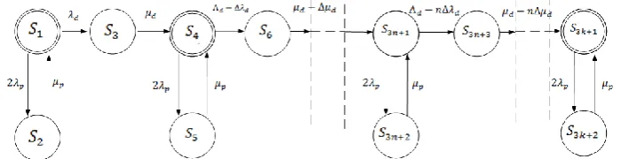
The Markov transition graph for the system presented in Fig. 1 is shown in Fig. 2. The model is built using the principle of multi-fragmentation [9]. Using this principle
the model can be divided into N fragments that are with the same structure but may
differ in one or more parameter values [21]. The number of fragments N in the MC
depends on the number of expected undetected software faults Nd, the value of which
can be estimated using probabilistic prediction models (6) [21]:
N=Nd+1 (6)
The sum of the failure rates of both software versions is defined as (7): Λd= λd (1) + λd(2) (7)
This MC of System 1 consists of the following states: SF1={S1, S4, …, Sn+1} – the
set of states when both the hardware and software on both channels are working correctly, SF2={S2, S5, …, S3n+2} – the set of states in which one of the hardware channel
has failed, SF3={S3, S6, …, S3n+3} – the set of states in which one of the software versions
has failed.
The system’s operation is described next. At time t0 the system operates correctly
in S1. At random moment, tn, a hardware or a software component failure occurs. In
case of a hardware failure the system moves to state S2. The rate of this transition is 2λp
and recovers from this state back to S1 with rate μp. In case of software failure the
system moves to state S3 and recovers from this failure by moving to state S4 with rate
μd. The states S1, S2 and S3 form the first fragment of the model, S4, S5 and S6 – form
fragment 2, etc. We assume that the internal fragments rates μd and Λd decrease by Δμd
and Δλd, respectively, as the system moves between fragments from left to right.
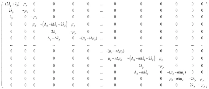
From the (Fig. 2) we derive the matrix of the system transition rates, where i=(1,..,n)
[image:10.595.122.472.511.601.2]is the number of system fragments:
(2 ) 0 0 0 0 ... 0 0 0 0 0 0 2 0 0 0 0 ... 0 0 0 0 0 0 0 0 0 0 ... 0 0 0 0 0 0 0 0 2 0 ... 0 0 0 0 0 0 0 0 0 2 0 ... 0 0 0 0 0 0 0 0 0 0 ( ) ... 0 0 0 0 0 0 ... ... ... ... ... ... ... ... ... ... ... ... ... 0 0 0 0 0 0 ... ( ) 0 0 0 0 0
p d p
p p
d d
d d d p p
p p
d d d d
d d i i n
0 0 0 0 0 0 ... 2 0 0 0 0 0 0 0 0 0 ... 0 2 0 0 0 0 0 0 0 0 0 ... 0 0 ( ) 0 0 0 0 0 0 0 0 ... 0 0 0 2 0 0 0 0 0 0 ... 0 0 0 0 2
d d d d p p
p p
d d d d
d d p p
p p n n n n n
System 2: A Queuing System with Server Breakdown and Repair. The second system was described in details by K.S. Trivedi and A. Bobbio in [4, 10]. The authors consider an M/M/1/k queuing system where m is the system capacity. The first “M” denotes a Poisson arrival process, the second “M” – denoted an exponentially distributed service times. The system has 1 server and k buffers to hold customers waiting for a service. The resulting model operates in 22 states [11]. Fig. 3 shows the Markov transition graph for the system.
0,0 2,0 m,0
1,1
0,1
1,0
[image:11.595.126.470.146.292.2]2,1 m,1
Fig. 3. The state diagram of the M/M/1/m queuing system with a server breakdown and repair Model parameters. The λ and μ are the arrival and the service rates, respectively, while γ and τ denote the server failure and failure repair rates. The main assumption is that the rates λ and μ are fast while γ and τ are slow [4]. Using the parameters presented in
[11] we computed the index of stiffness for this system to be s(x) =3·104. Under the
terms of this paper this system as classified as a high-stiffness system. The system was
solved on the same interval [0, 1000) [11].
3.2 Experimental Results
In this Subsection we present the results obtained using the approaches described in Section 2. The solutions for the MC of high-stiffness (the queuing system) is referred
to as Experiment 1. The solution for the MC of moderate-stiffness (the fault-tolerant
computer system) with changing parameters, would be referred to as Experiment 2.
so that the stiffness index has become low (s(x)=50). This solution will be referred to as Experiment 3.
Experiment 1. A solution of the queuing system with sever breakdown and repair using SAA was presented in [4], [11]. In [4] as a measure of interest the authors used the expected number of customers in the queue, E[N]. In [11], in addition, the approximate
result (calculated using SAA) and the exact values of P22(t) - the probability of having
all buffers full and the server down – were plotted together.
Now we turn our attention to solve the MC of high-stiff using the STA to solve this model. We used two methods that fall into the STA category:
- Using the EXPMETH utility
- Using the functions for solving stiff DEs implemented in the mathematical
package Mathematica.
We used EXPMETH with initial data as follows: the matrix of coefficients was set as defined in [11]; the mission time was set to t=1000; the accuracy of the solution
sought was set to 10-6; the number of steps was set to n=20. As Table 2 illustrates we
[image:12.595.125.473.367.469.2]obtained a negative result, where the probabilities were calculated for every 50 hours of the mission time, S={S1,S2,S3,…,S20}.
Table 2. Results obtained for Experiment 1 with ODU (EXPMETH)
Sn
t S1 … S20
50
1.76231646111739250e+0100-4.15365304345735515e+0100
1.06048815978458797e+0095-3.22465594380700072e+0094 …
1000
1.88981041657022775e+2054-4.45414711917994213e+2054
1.13720867698699733e+2049-3.45794216161554014e+2048
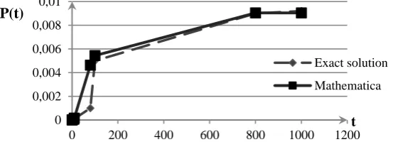
The results from using the functions for solving stiff DEs implemented in Mathematica
are summarised in Fig. 4 in which the exact solution for P22(t) for 𝜆1=1.0, given in [11],
is compared with the results obtained with Mathematica.
Based on the empirical evidence with the STA methods applied to Experiment 1 we
[image:12.595.147.424.546.646.2]conclude that STA cannot provide highly accurate solution for MCs of high-stiffness.
Fig. 4. Results of solving Experiment 1 model using Mathematica 0
0,002 0,004 0,006 0,008 0,01
0 200 400 600 800 1000 1200
P(t)
t
Exact solution
Experiment 2. To solve a moderately-stiff MC (Experiment 2) using SAA we used the algorithm described in [4] and the uniformization method. STA solutions are also obtained using EXPMETH and the mathematical package Mathematica, respectively.
The mission time was set again to t=1000, s(x)=4*102 (1), where max |Re(λ
i)|= 0.2
is the value of d, the software repair rate in the initial model fragment and
min|Re(λi)|=0.0005 is the value of d for the software repair rate in the final model
fragment.
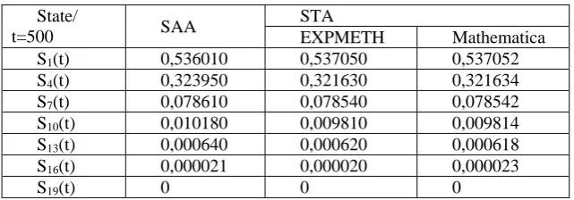
A comparison between the solutions is shown in Table 3 for values of the probabilities that the system is working in each of the states: {S1, S4, S7, S10, S13, S16,
S19} at t=500. This set represents the states without failure (operational states, i.e. both
[image:13.595.138.459.302.414.2]channels work correctly without hardware or software failure).
Table 3. Results comparison. System 1 State/
t=500 SAA
STA
EXPMETH Mathematica
S1(t) 0,536010 0,537050 0,537052
S4(t) 0,323950 0,321630 0,321634
S7(t) 0,078610 0,078540 0,078542
S10(t) 0,010180 0,009810 0,009814
S13(t) 0,000640 0,000620 0,000618
S16(t) 0,000021 0,000020 0,000023
S19(t) 0 0 0
Fig. 5 shows the results for system availability obtained with EXPMETH and Mathematica. For this system (Experiment 2) we used the result obtained with
EXPMETH as an exact solution [18]. A discussion of the discrepancies between the
solutions obtained with various packages is available in [18].
Based on this experiment we can conclude that for MCs of moderate - stiffness both the SAA and STA can be used. We note that the STA methods would produce an accurate solution faster than SAA when applied to small to moderate systems.
We also note that the particular mathematical package, Mathematica, detects automatically the stiffness of the DE’s using a built in “StiffnessTest”. In addition the user of this package can use ”StiffnessSwitching”, the basic idea as the name suggests being that the package will switch automatically between stiff and non-stiff solvers depending on the outcome of the stiffness test. The non-stiff solver uses the “ExplicitModifiedMidpoint” base method, while the stiff solver uses the “LinearyImplicitEuler” base method [22]. Such special methods can be useful in case of solving an MC of small to moderate size. Finally, we note that the mathematical package offers convenience, but at same time significant effort is required to construct the necessary functions in case of large models, which introduces scope for human errors, e.g. while entering the initial data.
EXPMETH can be more effective in terms of usability. With Experiment 2
Mathematica required a function with 7 arguments, while EXPMETH only required 4 arguments and a matrix of coefficients of the DEs.
Fig. 5. Comparison of STA methods applied to Experiment 2
Experiment 3. We solved the model of a system with low-stiffness (Experiment 3) using the STA only. Based on the justification in Subsection 2.1 we concluded that SAA are the best for solving MCs of high-stiffness and large MCs of moderately-stiffness. In case of MCs of low-stiffness the use of STA can take less time and still provides an accurate solution. As in the previous experiment we consider a mission
time t=1000, the s(x)=50 (1), where max |Re(λi)|= 0.2 – the value of d software repair
rate in the initial model fragment and min|Re(λi)|=0.004 – the value of d software
repair rate in the final model fragment. Fig. 6 shows the results of the comparison of
system availability, Pa(t), obtained with EXPMETH and Mathematica. The results are
practically indistinguishable. Based on this experiment we can conclude that for MCs of low-stiffness the STA can provide an accurate result.
Fig. 6. Comparison of results with STA methods applied to Experiment 3
4
Selection of a Solution method and of a Software Tool
Based on the results presented in the previous Subsection we propose the following selection procedure (Fig. 7), which takes into account the index of stiffness of the MC
under consideration. The first layer of the algorithm takes the index of stiffness, s(x)
given by (1), as an initial separator. The system in question is assigned to one of the three classes: high-stiffness, moderate-stiffness or low-stiffness.
An MC of high-stiffness.If the value of s(x) is greater or equal than 103 the system
model is defined as an MC of high-stiffness. We move to the left branch of the algorithm. If in the system under consideration the parameters change over time, we propose that the principle of multi-fragmentation (MFM) be used. Otherwise this step is skipped.
0,92 0,94 0,96 0,98 1
0 2000 4000 6000 8000
EXPMETH
Mathematica
0,94 0,96 0,98 1
0 200 400 600 800 1000
P(t)
t
EXPMETH Mathematica P(t)
[image:14.595.146.429.416.513.2]parameters
variation parameters variation
parameters variation
Build the MFM
Build the MFM
Build the MFM
Yes Yes Yes
Use the IMC
Use the IMC
Use the IMC
No No No
Use of SAA
Special tools use
Moderate value 102< s(x) <103
s(x) ≥103
High value Low value
s(x) ≤ 102
Large MC Yes
No
Use of STA
Use ODU or
special tools Special tools use
Yes No
Use of STA
Use of
math-tools
Use ODU, special tools or math-tools Begining
Solved stiff IMC
End
Large MC
Use of STA Use of
[image:15.595.126.470.136.567.2]SAA Initial stiff MC
Fig. 7. An algorithm of selecting an optimal method for solving MCs based on the stiffness index and the size (largeness) of an MC
Based on the results from Experiment 1, we propose that SAA be used. In this case
using specialized software will provide the most accurate solution. The use of STA in this case can produce a solution of low accuracy, which may be unacceptable.
An MC of moderate-stiffness. If the index of stiffness is in the interval [102, 103] we
As a theoretical separator the number of system states n=1000 can be used. If the
number of model states is greater than n – the model is considered large, otherwise the
model is not large. To provide effective results in case of a moderately-stiff large MC we propose the use of SAA and specialized tools. Indeed, one of the main features of SAA is the reduction of the system state space. For moderately-stiff MCs which are not
large, based on the results of Experiment 2, we propose that STA be used with either
EXPMETH or other specialized tools.
An MC of low-stiffness.If the index of stiffness is low, s(x) ≤ 102, we move to the
right branch of the algorithm. On the second layer we use the same separator as in previous cases. If the system under consideration includes parameter changes then MFM is needed, otherwise it is not needed and the initial MC can be used. In the third layer the system largeness is used as a separator. In case of a large MC of low-stiffness we propose that STA be used; as a tool we would recommend either EXPMETH or another specialized tool. These specialized tools were developed for special problems solution so they can provide more convenient data representation and satisfy the requirements of high accuracy. In the case of an MC of low-stiffness which is “not large” we propose the use of STA and EXPMETH or mathematical packages.
5
Conclusion
As a result of empirical studies we noticed that the value of stiffness index and the size of the MCs can affect the accuracy of the solutions achievable using different methods. One of the interesting results is that we can effectively use the SAA to solve a large moderately-stiff MC when the parameters vary, which was the focus in previous research work [18]. In our future work we intend to extend the algorithm presented in the paper and take into account the most effective approach that can deal with large MCs: largeness-tolerant and largeness-avoidance approaches. As a result we are hoping to define the best combination of “largeness-stiffness” approaches that can be applied effectively to systems with variable parameters.
6
References:
1. Volkov, L.: Managing the operation of the aircraft systems: Tutorial. Vyshaya
Shkola, Moscow (1981). “(In Russian)”
2. Ventsel', E., Ovcharov, L.: Probability theory and its applications in engineering.
Nauka, Moscow (2000). “(In Russian)”
3. Archana, S., Srinivasan, R., Trivedi, K.S.: Availability Models in Practice.
Proceedings of Int. Workshop on Fault-Tolerant Control and Computing (FTCC-1), May 22-23, Seoul, Korea (2000).
4. Bobbio, A., Trivedi, K.S.: A aggregation technique for transient analysis of stiff
Markov chains. In: Computers, IEEE Transactions, vol. C-35, pp. 803-814 (1986)
5. Malhotra, M., Muppala, J.K., Trivedi, K.S.: Stiffness-tolerant methods for
6. Arushanyan, O., Zaletkin, S.: Numerical solution of ordinary differential equations using FORTRAN. Moscow State University, Moscow (1990). “(In Russian)”
7. Bank, R.E. et al.: Transient simulation of silicon devices and circuits. In: IEEE
Transactions on Electron Devices, 32(10):1992-2007, (1985)
8. Geist, R., Trivedi, K.S.: Reliability estimation of fault-tolerant systems: tools and
techniques. In: Computer. Vol. 23, pp. 52-61, (1990)
9. Kharchenko, V., Timonkin, G., Sychev, V.: Fundamentals of design and
constructions the automated control systems for aircraft technical state control. Study guide. KVKIU, Kharkov (1992). “(In Russian)”
10. Nicola, V.F.: Markovian models of transactional system supported by check
pointing and recovery strategies, part 1: A model with state-dependent parameters. In: Eindhoven Univ. Technol., Eindhoven, The Netherlands, EUT Rep. 82-E-128, (1982)
11. Reibman A., Trivedi K. S., Kumar S., Ciardo G.: Analysis of stiff Markov chains.
In: ORSA Journal on Computing, vol. 1, No.2, pp. 126-133, (1989)
12. Hayrer, E., Vanner, G.: Solution of ordinary differential equations. Stiff and
differential-algebraic problems. Mir, Moscow (1999). “(In Russian)”
13. Press, W.H, Teukolsky S.A., Vetterling W.T., Flannery B.P.: Numerical recipes.
The art of scientific computing, 3rd edition. Cambridge university press. p. 1262,
(2007)
14. Reibman, A., Trivedi, K.S.: Numerical Transient Analysis of Markov models. In:
Comput. Opns. Res., vol. 15, No. 1, pp. 19-36. (1988)
15. Jensen A.: Markoff chains as an aid in the study of Markoff processes. In: Skand.
Aktuarietidskrift, vol. 36, pp. 87-91, (1953)
16. Fox, B.L., Glynn, P.W.: Computing Poisson probabilities. In: Commun, ACM
31(4), pp. 440-445, (1985)
17. Miranker, L.: Numerical Methods for stiff equations and Singular Perturbation
Problems. In: D. Reidel, p. 218, Dordrecht, Holland (1981)
18. Kharchenko, V., Popov, P., Odarushchenko, O., Zhadan, V.: Empirical evaluation
of accuracy of mathematical software used for availability assessment of fault-tolerant computer systems. RT&A #03(26). vol. 7. pp. 85- 97 (2012)
19. Littlewood, B., Popov, P., Strigini, L.: Modelling software design diversity - a
review. In: ACM Computing Surveys. vol. 33, No1. pp. 177 - 208., (2001)
20. Popov, P., Manno, G.: The Effect of Correlated Failure Rates on Reliability of
Continuous Time 1-Out-of-2 Software. In: Computer Safety, Reliability, and Security (SAFECOMP 2011). Naples, Italy: Springer. (2011)
21. Kharchenko, V., Odarushchenko, O., Ponochovny, Y., Zhivilo, S., Odarushchenko,
E., Kharibin, O., Odarushchenko, V. High availability systems and technologies. Lectures. Kharchenko, V. (ed.). In: National aerospace university “KhAI”, p. 249 (2012)
22. Wolfram Mathematica 9 Documentation Center,