Adjustment of wind farm power output through flexible turbine operation using wind farm control

DOI: 10.1002/we

RESEARCH ARTICLE

Adjustment of wind farm power output through flexible

turbine operation using wind farm control

Sung-ho Hur1_{and William E. Leithead}1

1_{Department of Electronic and Electrical Engineering, University of Strathclyde, Glasgow G1 1XW, UK}

ABSTRACT

When the installed capacity of wind power becomes high, the power generated by wind farms can no longer simply be that dictated by the wind speed. With sufficiently high penetration, it will be necessary for wind farms to provide assistance with

supply-demand matching. The work presented here introduces a wind farm controller that regulates the power generated

by the wind farm to match the grid requirements by causing the power generated by each turbine to be adjusted. Further benefits include fast response to reach the wind farm power demanded, flexibility, little fluctuation in the wind farm power

output and provision of synthetic inertia. Copyright c2014 John Wiley & Sons, Ltd.

KEYWORDS

wind farm power control; wind turbine control; flexible turbine operation.

Correspondence

S. Hur, Department of Electronic and Electrical Engineering, University of Strathclyde, Glasgow G1 1XW, UK. E-mail:

hur.s.h@ieee.org

Contract/grant sponsor

Supergen Wind Energy Technologies Consortium/Engineering and Physical Sciences Research Council

Contract/grant number EP/H018662/1

Received . . .

1. INTRODUCTION

The 2013 statistic publication [1] by the European Wind Energy Association (EWEA) reports that there are 117.3 GW of installed wind energy capacity in the European Union (EU). With high penetration of wind power, the power generated by

wind farms can no longer simply be that dictated by the wind speed. The operation of somewind turbinesis already being curtailed [2,3]. It will be necessary forwind farmsto provide services to the grid including spinning reserve, frequency

support and assistance with supply-demand matching. In these circumstances, to regulate the power generated by the wind

farm to match the grid requirements, a wind farm controller, causing the power generated by each turbine to be adjusted, is required. A detailed survey on the recent development of wind farm control can be found in [4]. It is stated in the paper

Network Wind Farm Controller (NWFC)

Turbine Wind Farm Controller (TWFC)

Wind Farm

...

N : number of turbines : flags

: wind farm status : additional (+/- ve) power : unadjusted power : adjusted power (by PAC) Network Inputs

: :

Wind farm status

+ _

.

Figure 1.The structure of the wind farm controller.

the wind turbines. A flexible, hierarchic, decentralised and scalable approach to wind farm control that is pertinent to both

the categories is introduced here. It is capable of providing fast and accurate control of the power generated by the wind farm in the below and above rated wind speed without compromising the turbines’ own full envelope controllers through

enclosing them in an additional feedback.

The structure of the wind farm controller is shown in Figure1. It has two elements, the Network Wind Farm Controller (NWFC) and the Turbine Wind Farm Controller (TWFC). The NWFC acts on information regarding the state of the power

network to determine the required power output from the wind farm and so the adjustment (∆P) relative toPm, the wind speed dictated output that would arise with no adjustment. The TWFC acts on information regarding the state of the wind

farm and the turbines therein to allocate adjustments to each turbine,∆Pi(fori= 1, . . . , N, whereNis the number of turbines in the farm) relative to the wind speed dictated output of turbinei.

Each wind turbine in the farm has its own full operational envelope controller [7] that ensures the wind turbine follows its required operating strategy and remains in a safe operating condition through regulating rotor speed, torque and some

loads. Since the wind farm controller requires each turbine to adjust its power output on request, the full envelope controller is modified by addition of a Power Adjusting Controller (PAC) [8]. The summary of the PAC is included in AppendixAof

this paper. As described in the appendix, the PAC causes the turbine to adjust its generated power by a demanded amount

relative to that dictated by the wind speed. As the PAC is essentially a feed-forward controller, jacketing the full envelope controller, it does not compromise the operation of the full envelope controller. Hence, redesigning or retuning of the

existing full envelope controller is not necessary. Furthermore, the PAC is sufficiently fast acting to provide the turbine with a synthetic inertia response [9,10], but that usage of the PAC is not discussed in this paper.

To prevent the introduction of feedback loops between the wind farm controller and the individual turbines as depicted in Figure1, the only communication regarding the state of each turbine to the wind farm controller is through “flags”,

fi(fori= 1, . . . , N). Furthermore, since the wind farm consists of a large number of turbines, the wind farm controller feedback acting on the total power output from the farm only introduces very weak feedback on each turbine. That is, as

the number of turbines that share the adjustments to the wind farm power output increases, the feedback effect decreases,

causing the wind farm controller to act independently from the controllers of the wind turbines.

The purpose of this paper is to investigate the design and performance of the wind farm controller in Figure1with

50 60 70 80 90 100 110 120 130 140 0

0.5 1 1.5 2 2.5 3 3.5 4 4.5

5x 10 4

Generator speed (rad/s)

Generator Torque (Nm)

mode 2

mode 1

mode 3 mode 4

red

amber

green

Figure 2.Design operating curve and operating regions (i.e. red, amber and green zones) defined by the thresholds over the full envelope operation on the torque/speed plane.

by applying the wind farm controller to a wind farm model. The wind farm is modelled using both Matlab/SIMULINKR

and DNV GL Bladed (BLADED). The turbines are the Supergen (Sustainable Power Generation and Supply) Wind 5

MW exemplar wind turbine. The performance of the wind farm controller is analysed in more detail (e.g. in the frequency domain) in Section4, and conclusions are drawn in Section5.

2. WIND FARM CONTROL STRATEGY

The wind farm controller requires that each variable-speed pitch-regulated wind turbine be equipped with an existing full

envelope controller and PAC. The full envelope controller causes the turbine to track its design operating curve as depicted on the torque/speed plane in Figure2; that is, a constant generator speed (i.e. 70 rad/s) is maintained in the lowest wind

speeds (mode 1); the Cpmaxcurve is tracked to maximise the aerodynamic efficiency in intermediate wind speeds (mode

2); another constant generator speed (i.e. 120 rad/s) is maintained in higher wind speeds (mode 3); and in above rated wind speed, the rated power of 5 MW is maintained by active pitching (mode 4) [11,12].

The PAC provides fully flexible operation adjusting the power output from each turbine, more specifically, reducing the power for an unlimited time or increasing the power for a limited time if required, without altering the dynamics of the full

envelope controller. However, if an increase or decrease in the power output is sustained, the turbine operating state could move away from the design operating curve.

The wind farm controller regulates the wind farm power output ensuring, at the same time, that each turbine (with the full envelope controller and PAC) operates within the safe operating region defined by the thresholds in Figure2; that is,

each turbine is prevented from going into unacceptable area, i.e. red zone as depicted in the figure, by the use of thresholds.

In below rated wind speed, the turbines operating inside the inner thresholds, i.e. the green zone, could be allocated greater adjustments in power than the turbines operating outside the inner thresholds but inside the outer thresholds, i.e. the amber

In mathematical terms, these thresholds are determined on the generator torque (Te)/generator speed (ωg) plane [13] for

convenience as

yT =Te−kTω2g (1)

wherekTis a constant, unique for each threshold. For instance, with reference to the outer threshold (between the amber

zone and the red zone) above the design strategy curve,yTbecoming positive indicates that the threshold has been crossed and the turbine is operating in the red zone, and vice versa. Hysteresis loops are incorporated into the thresholds to avoid

chattering. Each hysteresis loop is asymmetric around the threshold, i.e. the distance from the threshold to the lower hysteresis limit is103_{(when switching from the red to amber zone) while the distance from the threshold to the upper}

hysteresis limit is 5 times larger (when switching from the amber to red zone) because it moves more rapidly from the amber to red zone than from the red to amber zone.

Based on these thresholds, flags are returned as 0, 1 orfm. For the case investigated, settingfmto 3 is suitable in modes

2, 3 and 4. In mode 1, the PAC is not activated. If a turbine is operating within the green zone (Figure2), a flag offm would be returned. If a turbine is operating within the amber zone, a flag of 1 would be returned. Finally, if a turbine is

operating within the red zone, a flag of 0 would be returned.∆Piwith a flag of 0 would be zero, and∆Piwith a flag of 3 would be 3 times larger than∆Piwith a flag of 1.

The generation of the flags should be performed within the PAC rather than outside the PAC. Therefore, the PAC has been modified from the version reported in [8], and it now includes the flag generation feature as discussed in this section.

The summary of the PAC included in AppendixAof this paper is up to date. Note that newer versions of the PAC should always include this feature. Other than this modification, the wind farm controller does not make any changes to the PAC;

that is, the rest of the wind farm controller is developed outside the PAC.

The wind farm status could be determined by a number of factors including the health, age and location of the turbines.

For instance, reduction in generated power may be made to only half the wind turbines in the farm, those on the up-wind

side of the farm. The wind farm status,fˆi(fori= 0,1, . . . , NT) is also returned as 0, 1 orfm. In turn,fˆiandfiare compared and the minimum is exploited in equation (4). However, it is assumed that every turbine has the same status in

this paper; that is,fˆi=fm(for alliand wherefm= 3for the case studied here).

The NWFC calculates∆P(in Figure1) using the following proportional-integral (PI) controller:

∆P(t) =kp(Pd(t)−P(t)) +ki

Z

(Pd(t)−P(t))dt (2)

subject to the actuator constraints, whereP(t)andPd(t)denote adjusted power and demanded power, respectively, and

kpandkiare the tuning parameters. The structure of the PI controller with anti-windup is depicted in Figure3. In order to

prevent integral windup,∆Pis limited to be less than 40 % of the rated power. Note that the PAC should not be utilised to curtail the power output by more than 30 % in real life [8].kain the figure is the tuning parameter for the anti-windup

loop.

Consequently, unadjusted power, Pm (the wind speed dictated wind farm power output that would arise with no

adjustment) would be

Pm=P−∆P (3)

The TWFC distributes∆Pto each turbine as∆Pibased on flags,fi(status of each turbine) andfˆi(wind farm status as depicted in Figure1) as follows

∆Pi=

∆Pmin(fi,fˆi)

PN_T

j=1min(fj,fˆj)

PI P_d- P

+ _{_}

k_a

P

_ +

Figure 3.PI controller with anti-windup.

fori= 1, . . . , N. The implication is that

NT

X

i=1

∆Pi= ∆P (5)

whereNTdenotes the number of turbines in the wind farm. Equation (5) ensures that the power output from the wind farm tracks the demanded power even when the flags, hence∆Pi, are being adjusted.

The allocation and reallocation of the power adjustment should take place in a smooth manner, which avoids the introduction of large transients, discontinuities and steps in the wind farm power output. It is achieved by filteringfi

(fori= 0,1, . . . , NT) to ensure that the smoothing occurs only when crossing thresholds; that is, filteringfiis equivalent to filtering∆Pionly when crossing thresholds. A low pass filter, with time constant of 3 s, is exploited although the time constant could be larger in real life.

The full envelope controller ensures that the switching between the various modes (Figure 2) also takes place in a

smooth manner.

3. SIMULATION RESULTS

Matlab/SIMULINKR

and BLADED models of the Supergen 5 MW exemplar turbine, whose rated wind speed is

approximately 11.5 m/s, are utilised. The Matlab/SIMULINKR

model includes modules of aerodynamics, blades

dynamics, rotor dynamics, actuator dynamics, drive-train, tower dynamics, generator, etc. and is reported alongside the full envelope controller in [7,14] – each turbine model includes the full details reported therein, rather than being simplified.

The parameters of the Supergen 5 MW exemplar turbine are used. The BLADED model provides greater details for the structural loads, while the Matlab/SIMULINKR

model enables many turbines to be included in a wind farm model. The

wind farm model thus consists of 9 Matlab/SIMULINKR

models and 1 BLADED model. The two software packages are connected using StrathControl Gateway, a commercial software package that fully integrates the simulation. Due to the

high computational demand, it is assumed that the wind farm contains only 10 turbines.

In this paper, as previously mentioned, it is assumed that every turbine has the same status except that they operate in

different wind speeds. The different wind speeds cause the turbines to operate on different parts of the design operating

curve (Figure2).

A number of simulations have been conducted to demonstrate how the wind farm control strategy performs, and three

always negative in just below rated wind speed that requires the full envelope controllers to switch between modes 2 and

3.

3.1. Wind Speed Model

The wind stochastically varies with time and continuously interacts with the rotor [15]. The effective wind speed is wind speed averaged over the rotor area such that the power spectrum of aerodynamic torque remains unchanged. In this paper,

it is derived by filtering the point wind speed [16] through the filter introduced in [15]. The point wind speeds that take account of the correlation of the cluster layout and the wake effects are obtained from Bladed, thereby ensuring that the

wind speeds are appropriately correlated. The effective wind speeds are required as inputs for the Matlab/SIMULINKR

models. Bladed models include comprehensive models of complex wind fields to excite the turbine model, and the effective

wind speed model is thus not required. By employing Bladed’s built-in option, it is ensured that the wind speed that excites

the turbine model is correlated with the effective wind speeds experienced by the Matlab/SIMULINKR

models.

10 turbines are assumed to be aligned normally to the wind direction and evenly spaced 1 km apart, and the Bladed

model represents the 5thturbine in the cluster. In Figure4, the correlated effective wind speeds at a mean wind speed of 8 m/s incorporated into the 9 Matlab/SIMULINKR

models (the Bladed model representing the 5thturbine) are depicted.

Similar results can be expected at different mean wind speeds. Turbulence intensity of 10% is employed throughout this paper.

100 150 200 250 300 350 400 450 6

6.5 7 7.5 8 8.5 9 9.5 10

time (s)

Wind speed (m/s)

1 2 3 4 6 7 8 9 10

Figure 4.Wind speeds for turbines 1, 2, 3, 4, 6, 7, 8, 9, 10 at a mean wind speed of 8 m/s.

3.2. Simulation 1

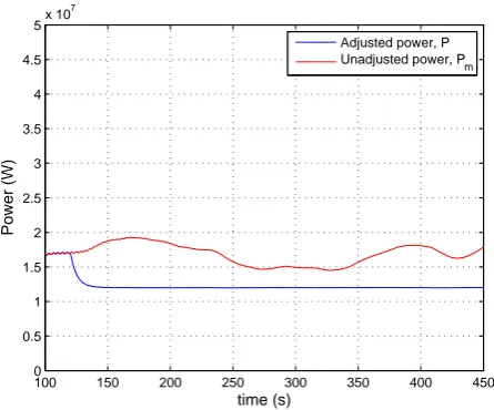
In Simulation 1, the wind farm is required to produce a constant power of 12 MW at a mean wind speed of 8 m/s. Adjusted

power in blue is depicted against unadjusted power in red in Figure5. The PAC is switched on at 120 s past the transient response, and∆P always remains negative.

Since it is the wind farm power output that is regulated, the individual power outputs from each turbine are still changing and being adjusted as depicted in Figure6. The turbines experiencing lower wind speeds, for much of the time, generate

less than 1.2 MW (demanded power output divided by the number of turbines,N), whilst those experiencing higher wind

speeds, for much of the time, generate more than 1.2 MW. In total, a constant wind farm power output of 12 MW is produced as depicted in blue in Figure5.

100 150 200 250 300 350 400 450 0

0.5 1 1.5 2 2.5 3 3.5 4 4.5

5x 10 7

time (s)

Power (W)

Adjusted power, P Unadjusted power, P_m

Figure 5.Simulation 1: adjusted vs unadjusted power.

100 150 200 250 300 350 400 450 0

1 2 3 4 5 6x 10

6

time (s)

Power (W)

P

1 P2 P3 P4 P5

100 150 200 250 300 350 400 450 0

1 2 3 4 5 6x 10

6

time (s)

Power (W)

P

6 P7 P8 P9 P10

Figure 6.Simulation 1: power outputs from each turbine.

100 150 200 250 300 350 400 450 0

1 2 3 4 5 6x 10

6

time (s)

Power (W)

P

1 P2 P3 P4 P5

100 150 200 250 300 350 400 450 0

1 2 3 4 5 6x 10

6

time (s)

Power (W)

P

6 P7 P8 P9 P10

Figure 7.Individual curtailment: curtailed power outputs from each turbine.

100 150 200 250 300 350 400 450 0.5

1 1.5

2x 10 7

time (s)

Power (W)

adjusted power by individual curtailment, P ind adjusted power by wind farm controller, P

Figure 8.Adjusted power by individual curtailment vs adjusted power by the wind farm control strategy.

50 60 70 80 90 100 110 120 130 140 0

0.5 1 1.5 2 2.5 3 3.5 4 4.5

5x 10 4

Generator speed (rad/s)

Generator Torque (Nm)

0.5 0.6 0.7 0.8 0.9 1 1.1 1.2 1.3 1.4 0

0.5 1 1.5 2 2.5 3 3.5 4 4.5

5x 10 6

Rotor speed (rad/s)

Aerodynamic torque (Nm)

Figure 9.Simulation 1: behaviour of each turbine on the torque/speed planes.

output from the wind farm would, for much of the time, be less than 12 MW as depicted in blue against the adjusted power by the wind farm controller in red.

The performance of each turbine can be observed from Figure9, which depictsTf (left sub-figure) andTe(right

sub-figure) on the torque/speed planes from 100 to 450 s. The results demonstrate that the turbines operate within the green zone, allowing for the hysteresis loop. In more detail, when a turbine switches from the green zone to the amber zone, the

turbine is allocated smaller adjustment in power, as the flag changes from 3 to 1, thereby causing the turbine to either slow down in moving towards the red zone or to return to the green zone. In this example, the turbines return to the green zone,

and the red zone is never reached.

Despite all the allocation and reallocation of∆P to each turbine as illustrated in Figures6and9, a constant power of 12 MW is still maintained with little fluctuation as depicted in Figure5.

3.3. Simulation 2

In Simulation 2, the wind farm is required to produce a constant power of 17 MW at a mean wind speed of 8 m/s. Adjusted power in blue is depicted against unadjusted power in red in Figure10. The PAC is switched on at 120 s past the transient

100 150 200 250 300 350 400 450 0 0.5 1 1.5 2 2.5 3 3.5 4 4.5

5x 10 7

time (s)

Power (W)

Adjusted power, P Unadjusted power, P_m

Figure 10.Simulation 2 when equations (4) and (5) are exploited; adjusted vs unadjusted power.

50 60 70 80 90 100 110 120 130 140 0 0.5 1 1.5 2 2.5 3 3.5 4 4.5

5x 10

4

Generator speed (rad/s)

Generator Torque (Nm)

0.5 0.6 0.7 0.8 0.9 1 1.1 1.2 1.3 0 0.5 1 1.5 2 2.5 3 3.5 4 4.5

5x 10

6

Rotor speed (rad/s)

Aerodynamic torque (Nm)

Figure 11.Simulation 2 when equations (4) and (5) are exploited; behaviour of each turbine on the torque/speed planes.

60 65 70 75 80 85 90 95 100 1 1.2 1.4 1.6 1.8 2 2.2 2.4 2.6 2.8

3x 10 4

Generator speed (rad/s)

Generator Torque (Nm)

60 65 70 75 80 85 90 95 100 1 1.2 1.4 1.6 1.8 2 2.2 2.4 2.6 2.8

3x 10 4

Generator speed (rad/s)

Generator Torque (Nm)

Figure 12.Left: zoomed version of Figure11(left) (before modification); right: zoomed version of Figure13(left) (after modification).

PAC rejects the request and places the turbine in the recovery mode setting the recovery flag to inform the wind farm

controller [8]. Consequently, equation (5) can only be satisfied for a limited period of time when producing an additional power output.

50 60 70 80 90 100 110 120 130 140 0

0.5 1 1.5 2 2.5 3 3.5 4 4.5

5x 10 4

Generator speed (rad/s)

Generator Torque (Nm)

0.5 0.6 0.7 0.8 0.9 1 1.1 1.2 1.3 1.4 0

0.5 1 1.5 2 2.5 3 3.5 4 4.5

5x 10 6

Rotor speed (rad/s)

Aerodynamic torque (Nm)

Figure 13.Behaviour of each turbine on the torque/speed planes.

100 150 200 250 300 350 400 450 0

0.5 1 1.5 2 2.5 3 3.5 4 4.5

5x 10 7

time (s)

Power (W)

Adjusted power, P Unadjusted power, P

m

Figure 14.Simulation 2: adjusted vs unadjusted power after the modification.

The performance of each turbine can be observed from Figure11, which depictsTf (left sub-figure) andTe (right sub-figure) on the torque/speed planes from 100 to 450 s. When turbine 1, for instance, enters the red zone,∆P1would

become zero to bring turbine 1 back to the green zone via the amber zone, and it would be in the recovery process [9]. Equation (4) causes∆Piof the remaining turbines to increase in order to compensate for turbine 1, i.e. trying to satisfy equation (5). As mentioned previously, the turbine operating state becomes much more sensitive when∆P is positive, and as a result, the remaining turbines would speed up moving towards the red zone (due to the increase in∆Pi). This process would repeat until every turbine cascades towards the red zone as depicted in Figure11. A zoomed version of the

left sub-figure of Figure11is depicted in Figure12(left sub-figure).

As every turbine is now going through the recovery process at the same time, a large dip inP is produced as depicted

producing an additional power output. Equation (2) is replaced with

∆P(t) =kp(Q(t)Pd(t)−P(t)) +ki

Z

(Q(t)Pd(t)−P(t))dt (6)

where

Q(t) =

PNT

j=1fi(t)

NTfm(t)

(7)

With this modification, if every turbine is operating within the green zone,Q(t)would be 1. If only one turbine enters the red zone (causing the turbine’s flag to be 0), while the remaining turbines are still operating within the green zone (each of the remaining turbines having a flag of 3),Qwould become(30−3)/30, reducing∆P by1/10in effect. This causes

P(t)to track the modified power demand,Q(t)Pd(t), instead ofPd(t). Equation (5) now becomes

NT

X

i=1

∆Pi=Q∆P (8)

only if∆Pis positive.

As a result of the modifications, when one turbine enters the amber zone in the same example, the remaining turbines do not attempt to compensate as depicted in Figure13(i.e.∆Piof the remaining turbines would not increase), no longer causing each turbine to cascade towards the red zone in succession. A zoomed version of the left sub-figure of Figure13

is depicted in Figure12(right sub-figure) in comparison to the result from the same example before the modification is

made (left sub-figure). The right sub-figure demonstrates that no turbine enters the red zone, and each turbine returns to

the green zone as soon as it enters the amber zone. Consequently, the time response is also improved as depicted in Figure

14, i.e., the large dip shown in Figure10is no longer present.

When∆P is negative such as in Sections3.2and3.4, the turbine operating state is not as sensitive to the change in

∆Pi. Moreover, negative∆Pdoes not necessitate any recovery process [8] afterwards, and therefore, equation (4) can be safely exploited, hence satisfying equation (5).

3.4. Simulation 3

In Simulation 3, the wind farm is required to produce a constant power of 25 MW at a mean wind speed of 10 m/s. At

this mean wind speed, the controller causes the turbines to switch between the Cpmaxtracking (mode 2) and the constant speed (mode 3) operations. Adjusted power in blue is depicted against unadjusted power in red in Figure15. The PAC is

switched on at 120 s past the transient response. The performance of each turbine can be observed from Figures16and17, which respectively depictTfandTeon the torque/speed planes.

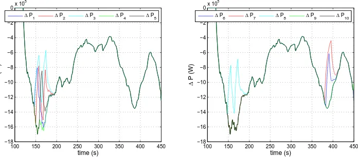
The left sub-figure of Figure16demonstrates the operation of each turbine from 100 to 450 s, and the right sub-figure (zoomed) the operation of turbines 1, 2, 6 and 7 only from 350 to 400 s. To analyse the simulation results in more detail,

attention is drawn to Turbines 1, 2, 6 and 7 in the right sub-figure. Turbines 1 and 2 operate in mode 3 while Turbines 6 and 7 operate in mode 2 just before 400 s. The figure depicts that Turbines 1 and 2 operate within the green zone while

Turbines 6 and 7 enter the amber zone. Consequently, Turbines 6 and 7 should be reallocated a reduced power adjustment

in comparison to Turbines 1 and 2. Figure18(just before 400 s) confirms that the reallocation takes place as expected at the switching region. As a result, turbines 6 and 7 re-enter the green zone as depicted in the figure.

100 150 200 250 300 350 400 450 0

0.5 1 1.5 2 2.5 3 3.5 4 4.5

5x 10 7

time (s)

Power (W)

Adjusted power, P Unadjusted power, P_m

Figure 15.Simulation 3: adjusted vs unadjusted power.

50 60 70 80 90 100 110 120 130 140 0

0.5 1 1.5 2 2.5 3 3.5 4 4.5

5x 10

4

Generator speed (rad/s)

Generator Torque (Nm)

100 105 110 115 120 125 1

1.5 2 2.5 3 3.5

x 104

Generator speed (rad/s)

Generator Torque (Nm)

P 1 P

2 P

6 P

7

Figure 16.Simulation 3: behaviour of each turbine on the (generator) torque/speed plane; left sub-figure: turbines 1 to 10 from 100 to 450 s; right sub-figure: turbines 1, 2, 3 and 4 only from 350 to 400 s for the same example (zoomed).

4. PERFORMANCE ASSESSMENT

The performance assessment of the wind farm controller is carried out in more detail here by exploiting the results from

simulation 3 in Section3.4. In Section4.1, mathematical proof and frequency analysis are presented to show that the

operation of the wind farm controller and that of the individual turbines’ full envelope controllers are independent. In Section4.2, how increase in the number of turbines in the wind farm affects the difference between the wind farm power

output and the power demand, which causes fluctuations, is examined. The speed of the wind farm controller is discussed in Section4.3, and the effect of the communication delay that exists between the TWFC and the wind farm, as depicted in

0.5 0.6 0.7 0.8 0.9 1 1.1 1.2 1.3 1.4 0

0.5 1 1.5 2 2.5 3 3.5 4 4.5

5x 10

6 T_f vs Ω

Rotor speed (rad/s)

Aerodynamic torque (Nm)

Figure 17.Simulation 3: behaviour of each turbine on the (hub) torque/speed plane.

100 150 200 250 300 350 400 450 −18

−16 −14 −12 −10 −8 −6 −4 −2

0x 10

5

time (s)

∆

P (W)

∆ P₁ ∆ P₂ ∆ P₃ ∆ P₄ ∆ P₅

100 150 200 250 300 350 400 450 −18

−16 −14 −12 −10 −8 −6 −4 −2

0x 10

5

time (s)

∆

P (W)

∆ P₆ ∆ P₇ ∆ P₈ ∆ P₉ ∆ P₁₀

Figure 18.Simulation 3: adjustment in power; left sub-figure: turbines 1 to 5; right sub-figure: turbines 6 to 10.

4.1. Decoupling of the wind farm controller from the wind turbines controllers

It is important to ensure that the wind farm controller does not create a significant feedback effect on the individual wind

turbine controllers. If a significant feedback effect is present, the effectiveness of the full envelope controllers could be

impaired. It would then require retuning of the wind turbine controllers, rendering the wind farm controller less practical. It is shown in this sub-section that the feedback does not affect the operations of the individual wind turbine controllers.

The decoupling of the wind farm controller from the wind turbine controllers could be confirmed mathematically as follows. The full envelope controller of turbine 1, for instance, is designed to produce power output,P1, to match the

demanded power,P˜1such that

P1= ˜P1 (9)

That is to say the equation is satisfied when the full envelope controller acts independently from the wind farm controller.

However, with the introduction of the wind farm controller, a feedback effect is also introduced, modifying the equation as

10−1 100 101 102 106

108 1010 1012 1014 1016

Frequency (rad/s)

PSD (Nm)

2/(rad/s)

Wind Farm Control 1 Turbine with feedback loop 1 Turbine with no feedback loop

Figure 19.Simulation 3: spectrum of fore-aft (My) tower bending moment (black) in comparison to the situations with (red) and without (blue) a feedback effect.

10−1 100 101 102 104

106 108 1010 1012 1014

Frequency (rad/s)

PSD (Nm)

2/(rad/s)

Wind Farm Control 1 Turbine with feedback loop 1 Turbine with no feedback loop

Figure 20.Simulation 3: spectrum of fore-aft (My) blade bending moment (black) in comparison to the situations with (red) and without (blue) a feedback effect.

assuming that∆Pfrom the NWFC is evenly allocated to each turbine,∆P1in equation (10) is replaced with∆P/N.

It is clear that if the wind farm controller acts on 1 turbine only, equation (9) is no longer satisfied, and the wind farm controller is not decoupled from the wind turbine controller. However, for a large number of turbines in the wind farm,

∆P/Nbecomes negligible and equation (9) is satisfied, i.e. the wind farm controller is decoupled from the wind turbine controller. Thus, the wind farm controller does not alter the effectiveness of the full envelope controllers for a wind farm

with a large number of turbines. Hence, the wind farm controller would be suitable for wind farms with a large number of turbines.

As previously mentioned, the decoupling of the wind farm controller from the wind turbine controller is further

enhanced as the only communication regarding the state of each turbine to the wind farm controller is through “flags”,

10−1 100 101 102 105

1010 1015

Frequency (rad/s)

PSD (Nm)

2/(rad/s)

Wind Farm Control 1 Turbine with feedback loop 1 Turbine with no feedback loop

Figure 21.Simulation 3: spectrum of side-side (Mx) blade bending moment (black) in comparison to the situations with (red) and without (blue) a feedback effect.

It is much more convenient to confirm that the decoupling is indeed present in the frequency domain than in the

time domain. In the time domain, the amplitude of any signal is dominated by the low frequency components making it problematic to discern any difference in behaviour at higher frequencies, where modifications to the full envelope controller

behaviour would be evident. Hence the difference that would arise as a result is shown much more clearly in the frequency domain than in the time domain. Moreover, a significantly larger set of data would be required in the time domain than in

the frequency domain.

For Simulation 3, the power spectra of fore-aft TBM, fore-aft BBM and side-to-side BBM are depicted in Figures19,

20and21, respectively. The spectra for the situations with (red) and without (blue) a feedback effect are also depicted for comparison purposes. To simulate the situation with a feedback effect, the wind farm controller is applied to a single

turbine model, and to simulate the situation without a feedback effect, a constant∆Pis applied with no feedback loop. The results demonstrate that the power spectra for the situation with the wind farm controller (applied to the 10 turbine

wind farm) and the power spectra for the situation with no feedback loop are analogous. It is, therefore, evident that

the wind farm produces a constant power of 25 MW at a mean wind speed of 10 m/s, avoiding creating any significant feedback effect even for a wind farm with only 10 turbines. It implies that the actions of the wind farm controller and the

wind turbine controllers are essentially independent. Almost identical results have been obtained for Simulations 1 and 2.

4.2. Increase in the number of turbines in the wind farm

Due to turbulence, the steady state power output adjusted by the wind farm controller would always fluctuate. Fluctuations,

Vr(t), due to the difference betweenP(t)andPd(t)(in %) is defined as

Vr(t) = 100

P(t)−Pd(t)

Pd(t)

(11)

whereP(t)andPd(t)denote adjusted power and demanded power, respectively.

Vr(t)for the 10 turbine wind farm is depicted againstVr(t)for a 5 turbine wind farm in Figure22; 5 turbine wind farm is only exploited to provide a comparison, and its demanded power output is reduced by half. The comparison demonstrates

100 150 200 250 300 350 400 450 −10

−8 −6 −4 −2 0 2 4 6 8 10

time (s) Vr

(%)

10 turbines 5 turbines

Figure 22.Fluctuations for 5 and 10 turbine wind farms for communication delay of 0.

10−1 100 101 102 10−6

10−5 10−4 10−3 10−2 10−1 100 101 102

Frequency (rad/s)

PSD (Nm)

2/(rad/s)

10 turbines 5 turbines

Figure 23.Spectra of fluctuations for 5 and 10 turbine wind farms for communication delay of 0.

10 turbine wind farm, while both the spectra exhibit similar characteristics. Hence, it could be inferred thatVr(t)would be almost negligible for a wind farm with many tens of turbines.

4.3. Speed of the wind farm controller

Power adjustment by the wind farm controller is caused by adjustments in generator torque and pitch angle. Figure24

illustrates that the adjustment in pitch angle takes place more slowly than the adjustment in torque (see [8]). Subsequently,

the wind farm controller filters the resulting power adjustment through a low pass filter for smooth transitions. Figure

25 demonstrates that the speed of the wind farm controller could be adjusted by altering the time constant. Although time constant of 3 s has been used throughout the paper for smooth transitions, it could be increased or decreased when

100 150 200 250 300 350 400 450 −16000

−14000 −12000 −10000 −8000 −6000 −4000 −2000 0

time (s)

Adjustment in torque (Nm)

100 150 200 250 300 350 400 450 0

0.02 0.04 0.06 0.08 0.1 0.12 0.14

time (s)

Adjustment in pitch angle (rad)

Figure 24.Adjustments in torque (left) and pitch (right).

100 150 200 250 300 350 400 450 0

0.5 1 1.5 2 2.5 3 3.5 4 4.5

5x 10 7

time (s)

Power (W)

time constant = 5 time constant = 1

Figure 25.Power adjustment at different speeds.

4.4. Communication Delay

The communication delay between the TWFC and the wind farm has been assumed to be zero throughout the paper. However, this may not always be feasible in real life. The impact of different communication delays, i.e. 0 s, 4 s (2 s each

way), 8 s (4 s each way) and 12 s (6 s each way), on the wind farm power output is depicted in Figure26.Vr(t)is still within 10 % for the largest communication delay of 12 s. It would be even smaller for a wind farm with a larger number

of turbines as depicted earlier in Figure22and eventually be negligible for wind farms with many tens of turbines; that is, large fluctuations in the wind farm power output would be avoided by ensuring that the number of turbines in the wind farm

is sufficiently large and that the communication delay is reasonably small (although the restriction on the communication delay can be relaxed as the wind farm size increases).

The performance of each turbine can be observed from Figure27, which depictsTe on the torque/speed plane for

different communication delays. As communication delay increases, the reaction time to the changes in flags increases, causing the turbines to operate outside the green zone more frequently. Nonetheless, the turbines still operate within the

100 150 200 250 300 350 400 450 2 2.2 2.4 2.6 2.8 3 3.2 3.4 3.6 3.8

4x 10 7

time (s)

Power (W)

Delay = 0 =2+2 =4+4 =6+6

Figure 26.Adjusted power for different communication delays.

50 60 70 80 90 100 110 120 130 140 0 0.5 1 1.5 2 2.5 3 3.5 4 4.5

5x 10

4

Generator speed (rad/s)

Generator Torque (Nm)

Delay = 0

50 60 70 80 90 100 110 120 130 140 0 0.5 1 1.5 2 2.5 3 3.5 4 4.5

5x 10

4

Generator speed (rad/s)

Generator Torque (Nm)

Delay = 2+2

50 60 70 80 90 100 110 120 130 140 0 0.5 1 1.5 2 2.5 3 3.5 4 4.5

5x 10

4

Generator speed (rad/s)

Generator Torque (Nm)

Delay = 4+4

50 60 70 80 90 100 110 120 130 140 0 0.5 1 1.5 2 2.5 3 3.5 4 4.5

5x 10

4

Generator speed (rad/s)

Generator Torque (Nm)

Delay = 6+6

Figure 27.Behaviour of the turbines for different communication delays.

Power spectra of fore-aft TBM, side-to-side BBM and fore-aft BBM are depicted for different communication delays

10−1 100 101 102 106

108 1010 1012 1014 1016

Frequency (rad/s)

PSD (Nm

2/rad/s)

Delay = 0 =2+2 =4+4 =6+6

Figure 28.Spectra of fore-aft tower bending moment for different communication delays.

10−1 100 101 102 104

106 108 1010 1012 1014

Frequency (rad/s)

PSD (Nm

2/rad/s)

Delay = 0 =2+2 =4+4 =6+6

Figure 29.Spectra of fore-aft blade bending moment for different communication delays.

5. CONCLUSIONS

A flexible, hierarchic, decentralised and scalable wind farm controller, capable of providing fast and accurate control of

the wind farm power output to meet the wind farm power demand as determined by the grid side operation requirements for the wind farm, is introduced. It utilises an existing full envelope controller and the PAC that has been developed to

provide fully flexible operation of an individual turbine. The wind farm controller, by the use of the PAC, causes the power generated by each turbine to be adjusted to regulate the wind farm power output to match the grid requirements, taking

into account the status and the operating state of each turbine. The operating state of each turbine is assumed to be equal

in this paper.

The simulation results in Matlab/SIMULINKR

and BLADED demonstrate that the wind farm power output could

10−1 100 101 102 105

1010 1015

Frequency (rad/s)

PSD (Nm

2/rad/s)

Delay = 0 =2+2 =4+4 =6+6

Figure 30.Spectra of side-to-side blade bending moment for different communication delays.

power adjustments between the turbines takes place in a smooth manner, which avoids the introduction of large transients,

discontinuities and steps in the wind farm power output. Hence, the resulting power output is smooth.

By curtailing the wind farm power output as opposed to curtailing individual turbine power outputs independently from

each other, improved results are attained by allowing those turbines seeing higher wind speeds to compensate for those

turbines seeing lower wind speeds. The wind farm controller is also utilised for providing additional power output for a limited period of time. When providing an additional power output, the control algorithm of the wind farm controller is

modified for improved results; that is, the turbines cascading towards the red zone is prevented by imroving the algorithm in Section 3.3.

The wind farm controller is also analysed in the frequency domain utilising power spectra to demonstrate that the wind farm controller does not cause a significant feedback effect that could compromise the effectiveness of the turbines full

envelope controllers. A simple mathematical proof is also presented. With a larger number of turbines in the wind farm, the feedback effect becomes even weaker. The simulation results also demonstrate that the impact of the communication

delay on the operation of the full envelope controller is small. The communication delay needs to be substantially large to cause considerable fluctuations (i.e.Vr(t)from equation (11)) in the wind farm power output, especially for a wind farm with a larger number of turbines. It is also illustrated that the speed of the wind farm controller could readily be altered,

which would be essential when providing the turbines with a synthetic inertia response, for instance.

ACKNOWLEDGEMENT

The authors wish to acknowledge the support of the EPSRC for the Supergen Wind Energy Technologies Consortium, grant number EP/H018662/1. The authors are grateful to Adam Stock for providing the PAC and a contribution to Appendix A

A. POWER ADJUSTING CONTROLLER RULES

The PAC supervisory rules are implemented in the PAC to ensure that the turbine is kept in a safe operating regime. The

occurrence of events triggered by these rules is communicated between the PAC and wind farm controller using flags. (Capital letters are used to indicate flag names with sub-flags in brackets.) There are two sets of rules, black rules defined

by a boundary on the torque/speed plane that act as a hard limit and traffic light rules, defined by two concentric boundaries contained within the black rules boundary, that act as soft limits. The boundaries apply to both aerodynamic torque and

drive-train torque. The regions inside the inner boundary, between the inner and outer boundaries and outside the outer

boundaries are designated green, amber and red, respectively. General supervisory rules:

• To turn off the PAC, the OFF flag is set by either the PAC or the wind farm controller and the PAC goes into

recovery mode. The speed of the recovery can be fast or slow as chosen by the wind farm controller through setting the RECOVERY (Fast/Slow) flag. The default is RECOVERY (Fast). During the recovery mode, the REJECTION

(Recovery) flag is set by the PAC.

• Only black supervisory rules apply to high priority events, such as requests for synthetic inertia. The PRIORITY

flag is set by the wind farm controller.

• During high turbulence intensity, the PAC is turned off and the REJECTION (Turbulence) flag set by the PAC. • If actuator pitch rate limits are violated by the turbine full envelope controller, the PAC is turned off and the

REJECTION (Actuator) flag set by the PAC with no time limit applied.

• If the turbine state is unstable such that normal operation is unreachable, the UNSTABLE flag is set by the PAC.

Black supervisory rules:

• The boundary and fixed upper limits to the demanded change in power are set with agreement and cannot be changed

without agreement of OEM.

• The boundary cannot be crossed under any circumstances.

• On the turbine state reaching the boundary, REJECTION (Limit) flag is set.

• If the turbine state remains on the boundary beyond the pre-set time limit then the PAC is turned off and the PAC

goes into RECOVERY mode.

• On a section of the boundary corresponding to the maximum possible generator reaction torque, the permitted time limit before turning off the PAC is zero.

Traffic light supervisory rules:

• The boundaries can be set by wind farm controller.

• The maximum change of power for the red region is zero. Subject to the fixed upper limit, the maximum change of power for the green and amber regions can be set by the wind farm controller with the latter less than the former. • When the turbine state is in the green/amber/red region, the GREEN/AMBER/RED flag is set by the PAC. • When the demanded change in power exceeds the maximum, the GREEN (Limit)/AMBER (Limit)/RED (Limit)

flag is set by the PAC.

REFERENCES

1. The European Wind Energy Association. Wind in power: 2013 European statistics.Technical Report, The European Wind Energy Association 2014.

3. Kristoffersen JR. The Horns Rev Wind farm and the Operational. Experience with the Wind Farm Main Controller.

Copenhagen Offshore Wind 2005, 26-28 October, 2005.

4. Knudsen T, Bak T, Svenstrup M. Survey of wind farm control–power and fatigue optimization.Wind Energ.2014;

:1–19.

5. Schepers JG, van der PSP. Improved modelling of wake aerodynamics and assessment of new farm control strategies.

Journal of Physics: Conference Series 752008; .

6. Jeong Y, Johnson K, Fleming P. Comparison and testing of power reserve control strategies for grid-connected wind

turbines.Wind Energ.2014; .

7. Chatzopoulos A. Full Envelope Wind Turbine Controller Design for Power Regulation and Tower Load Reduction. PhD Thesis, University of Strathclyde 2011.

8. Stock A. Flexibility of operation.Supergen wind energy technologies consortium report, Department of Electronics and Electrical Engineering, University of Strathclyde 2013.

9. Stock A. Providing grid frequency support using variable speed wind turbines with augmented control.Proceedings of the European Wind Energy Association (EWEA) Conference, Copenhagen, Denmark, 2012.

10. Gonzalez-Longatt F, Chikuni E, Stemmet W, Folly K. Effects of the synthetic inertia from wind power on the total system inertia after a frequency disturbance.2012 IEEE Power Engineering Society Conference and Exposition in

Africa (PowerAfrica)2012; :1–7.

11. Burton T, Sharpe D, Jenkins N, Bossanyi E.Wind Energy Handbook. John Wiley & Sons, Ltd, 2001.

12. Bianchi FD, Battista HD, Mantz RJ.Wind Turbine Control Systems: Principles, Modelling and Gain Scheduling

Design. Springer, 2006.

13. Leithead W, Connor B. Control of variable speed wind turbines: Design task.International Journal of Control2000;

73: 13:1189 – 1212.

14. Leithead W, Connor B. Control of variable speed wind turbines: Dynamic models.International Journal of Control

2000;73: 13:1173 – 1188.

15. Leithead WE. Effective wind speed models for simple wind turbine simulations.Proceedings of14th_{British Wind} Energy Association (BWEA) Conference, Nottingham, 1992.

16. Munteanu I, Bratcu AI, Cutululis NA, Ceang˘a E.Optimal Control of Wind Energy Systems: Towards a Global