When Micro Prudence Increases Macro Risk: The Destabilizing Effects of Financial Innovation, Leverage, and Diversification

      

City, University of London Institutional Repository

Citation

:

Corsi, F., Marmi, S. & Lillo, F (2016). When Micro Prudence Increases Macro Risk: The Destabilizing Effects of Financial Innovation, Leverage, and Diversification. Operations Research, 64(5), pp. 1073-1088. doi: 10.1287/opre.2015.1464

This is the accepted version of the paper.

This version of the publication may differ from the final published

version.

Permanent repository link:

http://openaccess.city.ac.uk/19451/

Link to published version

:

http://dx.doi.org/10.1287/opre.2015.1464

Copyright and reuse:

City Research Online aims to make research

outputs of City, University of London available to a wider audience.

Copyright and Moral Rights remain with the author(s) and/or copyright

holders. URLs from City Research Online may be freely distributed and

linked to.

City Research Online: http://openaccess.city.ac.uk/ [email protected]

When Micro Prudence increases Macro Risk: The Destabilizing

Effects of Financial Innovation, Leverage, and Diversification

Fulvio Corsi

∗

Stefano Marmi

†

Fabrizio Lillo

‡

October 20, 2015

Abstract

By exploiting basic common practice accounting and risk management rules, we

pro-pose a simple analytical dynamical model to investigate the effects of micro-prudential

changes on macro-prudential outcomes. Specifically, we study the consequence of the

introduction of a financial innovation that allow reducing the cost of portfolio

diver-sification in a financial system populated by financial institutions having capital

re-quirements in the form of VaR constraint and following standard mark-to-market and

risk management rules. We provide a full analytical quantification of the multivariate

feedback effects between investment prices and bank behavior induced by portfolio

re-balancing in presence of asset illiquidity and show how changes in the constraints of

the bank portfolio optimization endogenously drive the dynamics of the balance sheet

aggregate of financial institutions and, thereby, the availability of bank liquidity to the

economic system and systemic risk. The model shows that when financial innovation

reduces the cost of diversification below a given threshold, the strength (due to higher

leverage) and coordination (due to similarity of bank portfolios) of feedback effects

increase, triggering a transition from a stationary dynamics of price returns to a non

stationary one characterized by steep growths (bubbles) and plunges (bursts) of market

prices.

JEL classification: E51, G11, G18, G21.

Keywords: Systemic Risk, Diversification, Leverage, Endogenous Risk, Financial Innovation

∗_{Dipartimento di Scienze Economiche, Universit`a Ca’ Foscari, Venice, [email protected]} †_{Scuola Normale Superiore, Pisa, [email protected]}

‡_{Corresponding author. E-mail [email protected], Scuola Normale Superiore, Piazza dei Cavalieri 7,}

1

Introduction

In most standard economic models, financial institutions are viewed as passive players and

credit does not have any macroeconomic effect. Yet, a growing body of empirical literature

consistently finds that an acceleration of credit growth is the single best predictor of future

financial instability (see Gourinchas et al., 2001; Mendoza and Terrones, 2008; Borio and

Drehmann, 2009; Reinhart and Rogoff, 2009, 2011; Schularick and Taylor, 2012). These

empirical results confirm that the balance sheet dynamics of financial intermediaries, far

from being passive and exogenous, is instead the “endogenous engine” that drives the

boom-bust cycles of funding and liquidity and hence the dynamics of systemic risk. As stated by

Adrian and Shin (2010): “balance sheet aggregates such as total assets and leverage are the

relevant financial intermediary variables to incorporate into macroeconomic analysis”. In

fact, a change in the total assets of the financial institutions has important consequences

in driving the financial cycles through their influence on asset pricing, the availability of

credit, and funding of real activities. In this way changes in the total asset and leverage of

financial intermediaries play a key role in determining the level of real activity. However,

while the proximate cause for crises is very often an expansion of the balance sheets of

financial intermediaries the ultimate causes for these dynamics remain unclear.

In this paper, by exploiting basic common practice accounting and risk management

rules, we propose a simple analytical dynamical framework to investigate the effects of

micro-prudential changes on macro-micro-prudential outcomes. Specifically, we study the consequence of

the introduction of a financial innovation that allows reducing the cost of portfolio

diversifi-cation in a financial system populated by financial institutions having capital requirements

in the form of VaR constraint and following standard mark-to-market and risk management

rules. We provide a fully analytical description of the dynamics of the multivariate feedback

induced by portfolio rebalancing and trasmitted over the bipartite network of investment

prices and bank assets. We show quantitatively how changes in the constraints of the bank

portfolio optimization endogenously drive the dynamics of assets prices and that of the

bal-ance sheets of financial institutions and, thereby, the availability of bank liquidity to the

In building our model we try to keep behavioral assumptions at minimum, exploiting

instead the implications of “objective” constraints imposed by regulatory institutions and

standard market practice. We then start from a simple portfolio optimization problem in

presence of cost of diversification and VaR constraint1 showing how a reduction in the costs

of diversification (due, for instance, to financial innovations such as securization) leads to an

increase in both leverage and diversification.

So a first result is that financial innovation which, by increasing the optimal level of

diversification, reduces idiosyncratic risks, actually increases the exposure to undiversifiable

macro risks by increasing the optimal leverage of a VaR constrained investor. Moreover, a

higher level of diversification, by increasing the overlap among bank portfolios, increases the

correlation among them. Thus, the combined increase in risk exposure and correlation of

financial institutions will expose the economy to higher level of systemic risk.

We then link these results to the literature on the portfolio rebalancing induced by the

mark-to-market accounting rules and VaR constraint (see for instance Adrian and Shin

(2010); Greenwood et al. (2012); Duarte and Eisenbach (2013); Adrian and Shin (2014)).

In this balance sheet models an increase in the value of the assets, increases the amount

of equity leading to surplus of capital with respect to the VaR requirements which is

ad-justed by expanding the asset side through borrowing i.e. by raising new debt (typically

done with repos contracts). Hence, VaR capital requirements, induce a perverse demand

function: financial institution will buy more assets if their price rises and (with an

analo-gous mechanism but with reversed sign) sell more assets when their price falls. Therefore,

a VaR constrained financial institution will have positive feedback effect on the prices of

the assets in his portfolio.2 _{The intensity and coordination (among financial institutions) of}

these portfolio rebalancing feedbacks will depend, respectively, on the degree of leverage and

diversification.

In the second part of the paper, we then analyze the multivariate dynamics of the

endoge-1_{Note that VaR type of constraints arise from the capital requirements contained in Basel I and II bank}

regulations but also from margin on collateralized borrowing imposed by creditors (see Brunnermeier and

Pedersen 2008), rating agencies, and internal risk management models.

2_{This type of active balance sheet management is particularly utilized by investment banks, ABS issuers,}

nous asset price determined by the impact of supply and demand generated by the financial

institutions rebalancing their portfolio. The analytical results obtained in this second part of

the paper by applying the multivariate dynamic framework are manifolds: (i) higher overlap

induced by lower diversification costs increases both the variance and correlation of the

in-vestment demands of FIs rebalancing their portfolios; (ii) the feedback between inin-vestment

prices and bank asset induced by the multi-round portafoglio rebalances of VaR constrained

banks, leads to a multivariate VAR process whose maximum eigenvalue depends on the

de-gree of leverage and average illiquidity of the assets; (iii) lower level of diversification costs

or capital requirements can lead to dynamic instability of the system; (iv) the VAR process

can be represented as a combination of many idiosyncratic AR processes around a single

common AR process of the average values (i.e. the market); (v) the endogenous feedback

induced by portfolio rebalancing introduces an additional component to the variance,

covari-ance, and correlation of both the individual investment and the bank portfolios for which we

derive closed–form expressions; (vi) reduction in diversification costs monotonically increase

variance and correlation of individual investments thus acting as a “multiplier” of market

risk; (vii) the variance of portfolios shows, however, a non-monotonic relation with respect to

diversification costs; (viii) the endogenous feedback makes historical estimation of variance

covariance to be overestimated during periods of increasing leverage and underestimated

during periods of deleveraging thus providing a rationale for countercyclical capital

require-ments; (ix) in presence of endogenous feedbacks, an exogenous shock will trigger a sequence

of portfolio rebalances which will amplify its initial impact; (x) reduction in diversification

costs, by increasing the strength and coordination of individual feedbacks, increases the

variability of bank total asset, which governs the supply of credit and liquidity to financial

system

1.1

Related literature

In addition to the literature on the portfolio rebalancing induced by the mark-to-market

ac-counting rules and VaR constraint (Adrian and Shin, 2010; Greenwood et al., 2012; Duarte

and Eisenbach, 2013; Adrian and Shin, 2014) already mentioned, our paper tries to

requirements on the behavior of financial institutions and their possible procyclical effects

(Danıelsson et al., 2004; Danielsson et al., 2009; Adrian and Shin, 2009; Adrian et al., 2011;

Adrian and Boyarchenko, 2012; Tasca and Battiston, 2012); (ii) the literature on distressed

selling and its impact on the market price dynamics (Shleifer and Vishny, 1992; Kyle and

Xiong, 2001; Shleifer and Vishny, 2011; Cont and Wagalath, 2011; Thurner et al., 2012; Cont

and Wagalath, 2012; Caccioli et al., 2012); in particular, it extends the theoretical models

underpinning the systemic risk measure that quantifies the vulnerability of the financial

sys-tem to fire-sale spillover (Greenwood et al., 2012; Duarte and Eisenbach, 2013) to a dynamic

multi-round liquidity spillover framework; (iii) the literature on the effects of diversification

and overlapping portfolios on systemic risk (Wagner, 2011; Tasca and Battiston, 2011;

Cac-cioli et al., 2012; Lillo and Pirino, 2015); Differently from the paper of Wagner (2011) which

also proposes a model where higher level of diversification might increase aggregate risk, we

identify a different mechanism for this effect. In addition to the synchronization of portfolio

rebalancing among banks (as in Wagner 2011), we also consider the impact of diversification

costs on bank leverage and through that on the intensity of those portfolio rebalancing and

provide a fully analytical description of the resulting time series dynamics of assets prices

and bank total assets. (iv) the literature on the risks of financial innovation (Brock et al.,

2009; Caccioli et al., 2009; Haldane and May, 2011); (v) the literature on the determinants

of the dynamics of balance sheet aggregates and credit supply of financial institutions (Stein

1998, Bernanke and Gertler 1989, Bernanke, Gertler and Gilchrist 1996, 1999 and Kiyotaki

and Moore 1997).

Our contribution is to propose a simple model that, by combining these different streams

of literature, provides a fully analytical quantification of the links between micro prudential

rules and macro prudential outcomes in a multivariate context which considers both the

presence of endogenous feedback caused by portfolio rebalancing and the impact of financial

innovations on the cost of diversification.

The paper is organized as follows. Section 2 presents the model set up and the analytical

results by first describing the portfolio decision problem of financial institutions facing VaR

constraints and diversification costs and then analyzing its macroeconomic consequences in

Section 3 analyzes the systemic risk implications of our model both a static setting

with-out feedback and in a dynamic setting with the endogenous feedback generated by portfolio

rebalancing. Based on those analytical results, Section 4 discusses the macro-prudential

con-sequences of the introduction of financial innovations reducing diversification costs. Section

5 summarizes and concludes.

2

The model

2.1

Portfolio decisions

We begin by considering a financial institution endowed with a given amount of initial

equity capital E and we model its portfolio selection across a collection of risky investments

i= 1, ..., M. In general, these might be individual investments or asset classes. In order to keep the subsequent dynamic model fully analytical, we assume that, from the point of view

of the financial institutions, all the risky investments are ex-ante statistically equivalent.

As a consequence, financial institutions adopt a simple investment strategy consisting in

forming an equally weighted portfolio3 _{by randomly selecting m risky investments from the}

whole collection of M available investment assets.

Financial institutions, correctly perceive that risky investment entails both an

idiosyn-cratic (diversifiable) risk component and a systematic (undiversifiable) risk component, i.e.

the expected variance4 _{of the risky investment i, σ}2

i, can be decomposed as σ2i = σs2+σ2d

where σ2_s is the perceived systematic risk and σ_d2 is the perceived diversifiable risk compo-nent. Hence, the expected mean and volatility per dollar invested in the portfolio chosen by

a given institution are µand σp =

q

σ2

s + σ2

d

m, respectively.

Because of the presence of transaction costs, firms specialization and other type of

fric-3_{Theoretical and empirical advantages of the naive equally weighted strategy are provided in Benartzi and}

Thaler (2001); Pflug et al. (2012); DeMiguel et al. (2009); Tu and Zhou (2011). Equally weighted portfolios

are also popular among practitioners as they are robust to specification errors in the dynamics of individual

asset and provides performance in line (if no better) than those from more sophisticated Markowitz-type

approaches.

4_{Which, in general, might be different from the realized one since we remain agnostic on the process of}

tions, we assume the existence of “costs of diversification” (see Constantinides, 1986) which,

in general, can prevent each institution to achieve full diversification of its portfolio (precisely

the existence of these costs in real markets spurred the developments of financial innovation

products as we will discuss in the next sections).

Let rL be the per dollar average interest expense on the liability side, then the Net

Interest Margin (NIM) of the financial institution isµ−rL. The NIM is therefore a measure

of the overall profitability of a financial institution.

In line with the recent theoretical and empirical literature on bank behavior

(Brunner-meier and Pedersen, 2009; Adrian and Shin, 2010, 2014), financial institutions are confronted

with a Value at Risk (VaR) type of constraints. The VaR constraint is typically computed

as some multiple of the standard deviation of the portfolio of assets A.

With σp the expected holding period volatility per dollar of asset A and α a scaling

constant, the VaR constraint faced by the financial institution is

V aR=ασpA≤E. (1)

As empirically shown by Adrian and Shin (2010) financial institutions adjust their asset

side rather than raising or redistributing equity capital. In agreement with these empirical

observations, we will consider the equity capital of the financial institutions to be fixed.

Notice that this does not prevent the value of equity to change over time as in fact happens

as a consequence of the bank profits and losses. It only assumes that, in managing their

VaR capital requirements, financial institutions prefer buying and selling activities in their

asset sides rather than rising new equity or redistributing the one in excess.

Summarizing, given their NIM and level of equity E, financial institutions, facing cost of diversification and VaR constraints, choose the level of total asset A and degree of diversifi-cation m which maximize their returns from the risky investments. That is, assuming cost of diversification proportional to m, financial institutions maximize

max

A,m A(µ−rL)−cm˜ s.t. αA

r

σ2

s +

σ2

d

m ≤E. (2)

λ= A_E, max

λ,m λ(µ−rL)−cm s.t. αλ

r

σ2

s +

σ2

d

m ≤1. (3)

Hence, each institution chooses the optimal leverage λ∗ =A∗/E and the optimal number of investments m∗ which maximizes its Return On Equity (ROE) under its VaR constraints. It is convenient to transform the constraint by squaring both sides so that the Lagrangian

can be written as

L=λ(µ−rL)−cm−

1 2γ

α2λ2

σ_s2+ σ

2 d m −1 . (4)

whereγ is the Lagrange multiplier for the VaR constraint. The first order condition forλ is (µ−rL)−γα2σ2pλ = 0 ⇒ λ =

1

γ

1

α2

µ−rL

σ2

s + σ2_d m

(5)

Substituting in the constraint we obtain the Lagrange multiplier or shadow price of the VaR

constraint γ γ = 1

α

µ−rL

q σ2 s + σ2 d m = 1 α

µ−rL

σp

(6)

which is proportional to the Sharpe ratio. The optimal number of investments m∗ is then,

m∗ =

√

γαλσd

√

2c =λσd

s

α

2c

µ−rL

σp

(7)

which shows that, as expected, the level of diversification chosen is inversely related to the

cost of diversificationc. For the leverage we have,

λ∗ = 1

α q σ2 s + σ2 d m = 1 ασp (8)

thus, the optimal leverage is inversely related to the volatility of the asset portfolio. In the

following, we will drop the star symbol on the optimal values for notational convenience, i.e.

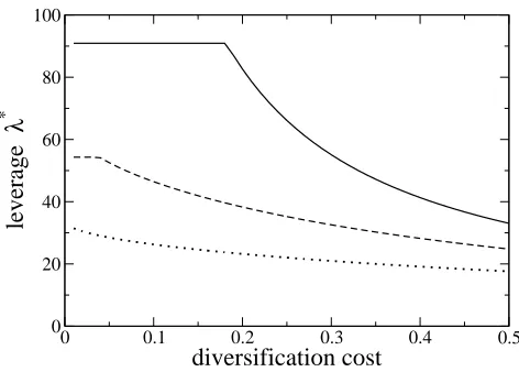
we will denote the target leverageλ∗ and diversificationm∗ simply as λand m, respectively. Figure 1 reports the numerical solutions for the optimal leverage as a function of different

levels of diversification costs (and for a given choice of the set of the remaining parameters

0 0.1 0.2 0.3 0.4 0.5

diversification cost

0 20 40 60 80 100

leverage

λ

[image:10.612.176.412.104.273.2]

∗

Figure 1: Relation between the optimal leverage λ∗ and the diversification cost c, obtained by solving numerically Eq.s (7) and (8). The used parameters are: M = 20, α = 1.64 (corresponding to a 5% VaR in a Gaussian setting), µ−rL = 0.08, σd = 0.03. We then

choose σs equal to 0 (solid line), 0.009 (dashed line), and 0.018 (dotted line).

ratio (σs/σd = {0, 0.3, 0.6}). A reduction of diversification costs, by increasing the level

of diversification and hence relaxing the VaR constraint, allows the financial institution to

increase the optimal leverage, especially for lower level of the systematic to idiosyncratic

noise ratio. Note that below a given cost the optimal leverage becomes constant due to the

saturation of diversification reached when the portfolio becomes perfectly diversified across

all the M available investments. The sensitivity of the optimal leverage to diversification costs is higher for lower systematic to idiosyncratic noise ratios.

2.2

Overlapping portfolios

We now assume that our economy is composed by a group ofN financial institutions labeled withj = 1, ..., N and investing in theM risky investments as described above. The portfolio holdings of the N banks can be represented by using a bipartite graph, where the first set of nodes is composed by the N banks and the second set of nodes is composed by the M

Duarte and Eisenbach 2013 and Di Gangi et al. 2015 for the properties of such network in

the US banking system).

As in the standard CAPM framework, we make the conventional assumption that banks

have homogeneous expectation over the investments assets and thus each bank solves a

simi-lar optimization problem identifying the same optimal degree of diversificationm. However, we will assume that each bank chooses randomly and independently the investments across

the set of the M available ones, so that the selected portfolios will be different for different banks. A realization of portfolio choices of all the banks leads to a specific instance of the

bipartite graph characterized by a N ×M matrix of portfolio weights W. In the following we will consider average values for these realizations of the bipartite graph configurations.

The number of banks n having a specific risky investment in their portfolio is a random variable described by the binomial distribution

P(n;N, M, m) =

N n

m

M

n 1− m

M

N−n

(9)

whose mean value is clearly E[n] =mN/M.

Taken two banks, we can define the overlap o of their portfolios as the number of risky investments in common in the two portfolios. Alsoois a random variable and it is distributed as an hypergeometric distribution

P(o;M, m) =

m o

M−m m−o

M m

0≤o≤m. (10) Its mean value is E[o] =m2/M and its variance isV[o] =m(M −m)2/(M2 −M). Finally, the fractional overlap of two portfolios of = o/m is a number between 0 and 1 describing

which fraction of the portfolio is in common between the two banks. Clearly, the mean

fractional overlap is ¯o ≡ E[of] =m/M, therefore the value of the portfolio size m is also a

measure of the average fractional overlap ¯o between portfolios and viceversa.

The left panel of Figure 2 shows the numerical solutions of the fractional overlap, coming

from the optimal portfolio decision, as a function of different levels of diversification costs

(again, each line corresponds to different levels of systematic to idiosyncratic noise ratio,

σs/σd = {0, 0.3, 0.6}). The figure shows how reducing the costs of diversification, by the

introduction of some new form of financial products for example, increases the degree of

0 0.1 0.2 0.3 0.4 0.5

diversification cost

0 0.2 0.4 0.6 0.8 1

portfolio overlap

0 0.5 1 1.5 2

α VaR

0 0.2 0.4 0.6 0.8 1

[image:12.612.94.503.102.242.2]

portfolio overlap

Figure 2: The left panel shows the mean fractional overlap ¯o between two portfolios versus the diversification cost c and the right panel shows ¯o versus the α parameter of the VaR constraint. (see Fig. 1 for the parameters). In the the right panel we setc= 0.25.

The fractional overlap resulting from the portfolio choices of financial institutions, can

also be represented as a function of the tightness of the imposed capital requirements. This

relation, depicted in the right panel of Figure 2, implies that regulator could tune the required

capital ratio α so to reach a given level of overlap, and hence correlation, among financial institutions.

2.3

Asset demand from portfolio rebalancing

Having identified their optimal leverage, financial institution periodically rebalance their

portfolios in order to maintain the desired target leverage. The rebalancing of the portfolio

of individual bankj at timet, is given by the difference between the desired amount of asset

A∗_j,t =λEj,t and the actual oneAj,t,5 i.e. ∆Rj,t ≡A∗j,t−Aj,t. By defining the realized return

portfolio r_j,tp , ∆Rj,t can be written as (see Appendix A)

∆Rj,t = (λ−1)A∗j,t−1r

p

j,t, (11)

that is, any profit or loss from investments in the chosen portfolio (r_j,tp A∗_j,t−1) will directly result in a change in the asset value amplified by the current degree of leverage (being

5_{As clearly shown by Adrian and Shin (2010), the balance sheet adjustments are typically performed by}

λ > 1). Hence, a VaR constrained financial institution will have a positive feedback effect on the prices of the assets in his portfolio.

The total demand of the risky investment i at time t will be simply the sum of the individual demand of the financial institutions who picked investment i in their portfolio.

Being more convenient to work with matrices and vectors, let us defineRttheM×1 vector

of investment returns andQt−1 =diag[(λ−1)A∗j,t−1] a N ×N diagonal matrix. Finally, let

us consider Wthe N ×M matrix of portfolio weights characterizing the banks-investments bipartite network. Then, the M ×1 vector of demandDt is

Dt =W0Qt−1WRt (12)

From this expression the linear character of the relation between the demand of each

invest-ment and the return of all other investinvest-ments is evident.

2.4

Risky asset dynamics with endogenous feedbacks

In this section we study the dynamics of the model in the case where the return of the

risky investments are endogenously influenced by the former period demands coming from

the portfolio rebalancing of financial institutions. In presence of rebalancing feedbacks, the

return process will now be made of two components:

ri,t =ei,t−1+εi,t (13)

the exogenous component εi,t coming from the external shocks and the endogenous

compo-nentei,t−1coming from the previous period portfolio rebalancing of the financial institutions.

We assume that the exogenous component has a multivariate factor structure

εi,t =ft+i,t, (14)

with the factor ft and the idiosyncratic noise i,t uncorrelated and distributed with mean

zero and constant volatility, respectivelyσf and σ (the same for all investments). Thus, the

variance of the exogenous component of the risky investmenti is V(εi) = σ2f +σ2.

return of investment iat time t becomes6

ei,t =

D_i,t γiCi,t

(15)

where Ci,t =

PN

j=1I{i∈j}

A∗_j,t−1

m is a proxy for market capitalization of investment i, and γi is

a parameter expressing the market liquidity of the investment i.

Given the homogeneity of investments, we can assume that all have the same market

capitalization which, since on average there are N m/M banks investing ini, is equal to

Ci,t 'Ct=

N M

¯

A∗_t−1 (16)

where ¯A∗_t−1 ≡N−1PN

j=1A

∗

j,t−1 is the average bank asset size (assumed to exist).

Substituting Equations (12), (13), and (16) in (15) and using matrix notation we

ob-tain the following Vector Autoregressive (VAR) dynamics of the vector of the endogenous

components

et =Φrt =Φ(et−1+εt) (17)

with

Φ≡ M

NA¯∗_t−1Γ

−1_W0

Qt−1W=

M NΓ

−1_W0_˜

QW (18)

where Γ is a M × M diagonal matrix with diagonal elements γi,i (the market liquidity

of investment i) and Q˜ = Qt−1/A¯∗t−1 a N ×N diagonal matrix with diagonal elements

˜

Qjj = (λj −1)A∗j,t−1/A¯

∗

t−1. The matrix Q˜ is assumed to be independent from t, since the

leverage is fixed and the fraction of total asset of a bank is assumed not to change in the

investigated period7_.

2.4.1 Random matrix approach

In order to proceed with the computation of the dynamical properties of returns, we take

expectations over the ensemble of the random matrices Wand study the model determined

6_{A stochastic component coming from the exogenous demands of traders not actively rebalancing their}

portfolio could be added at the cost of complicating the subsequent computations.

7_{These assumptions on the constancy of the matrixΓ andQ}˜ _{are invoked in order to obtain a standard}

VAR(1) with constant autoregressive matrix. They could be relaxed at the price of obtaining a dynamic

by the expectation of the matrix B≡W0QW˜ . Depending on the quantity of interest, this

approximation is more or less reliable and we later use numerical simulations to investigate

this point.

In order to have analytical tractability of the problem, from now on we assume that the

investment selection process is a series ofM independent Bernoullian draws each with prob-ability _Mm. The parameter m represents the average degree of diversification of portfolios8. In other words the number of investments of each bank is a Binomial variable with meanm

and, to keep the model general, we also assume that each bank has a leverage λj (possibly

related to the outcome of the Binomial).

Under these assumptionsWis then a random matrix where each entries is an independent

Bernoullian random variable Xj,i with probability m/M “normalized” by the sum sj =

P

iXj,i, i.e. each generic element of the matrix W is Wj,i= Xj,i

sj . Clearly,

P

iWj,i = 1.

The generic element of B is

Bij = N

X

k=1

˜

Qk,kWk,iWk,j. (19)

Being able to compute (see Appendix B)

E[W_k,i2 ]' 1

mM E[Wk,i, Wk,j]'

1

M2_c. (20)

We have,

E[Bii]'

1

mM

X

k

˜

Qkk E[Bij]'

1

M2_c

X

k

˜

Qkk, i6=j, (21)

where c≡1 + _m1 − 1

M.

In conclusion, the average matrix Φ¯ ≡E[Φ] of the VAR(1) is

¯

Φ'(¯λ−1)Γ−1Ψ with Ψ=

        1 m 1

M c . . .

1

M c

1

M c

1

m . . .

1 M c .. . . .. ... 1 M c 1

M c . . .

1 m         . (22)

8_{The choice of treating the diversification as a random variable simplifies the analytical computations. A}

model with fixed m can be developed analytically in a simplified and symmetric setting or, via numerical

simulations, in a general setting. It is possible to show that the conclusions of the papers do not depend on

where

¯

λ= PN

j=1λjA∗j,t−1

PN

j=1A

∗

j,t−1

(23)

is the asset weighted average leverage of the financial system. Notice that if all the banks

have the same leverage, the matrix Φ is independent from the bank asset size distribution

(provided the mean exists).

The dynamics of such VAR(1) process is determined by the eigenvalues of the matrix Φ¯.

The maximum eigenvalue ofΦ¯, dictating the dynamics of the VAR(1) process, becomes (see

Appendix C)

Λmax '(¯λ−1)γ−1 (24)

where γ−1 _{is the average of all the γ}−1

i . Hence, the maximum eigenvalue depends on the

degree of leverage and on the average illiquidity of the investments.

When the maximum eigenvalue is greater than one, the return processes become

non-stationary and explosively accelerating. It is important to remark that even a reduction

in the liquidity of only one risky investment (by changing the average illiquidity of the

investments) impacts the dynamics of all the traded investments and can potentially drive

the whole financial system towards instability. In fact, depending on the average of the _γ1

i,

the maximum eigenvalue (and thus the dynamical properties of the whole system) will be

highly sensitive to illiquid investments, i.e. to investment having a smallγ.

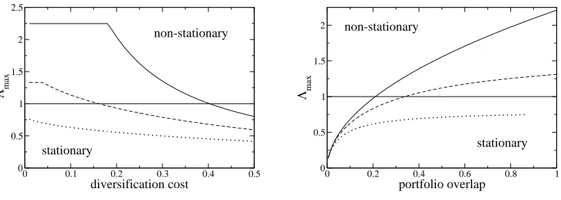
Figure 3 shows the maximum eigenvalue Λmax as a function of the diversification cost c

(left panel) and as a function of the mean portfolio overlap ¯o (right panel). We notice that a reduction of the diversification cost tends to reinforce the feedback induced by portfolio

rebalancing which can lead to dynamic instability of the system (for Λmax > 1) when the

diversification costs decrease below a certain threshold (which is higher for smaller ratio of

systematic to idiosyncratic volatility). Analogously, we can analyze the dependence of the

maximum eigenvalue of the dynamical system from the degree of portfolio overlap among

the financial institutions. A higher level of coordination in portfolio rebalancing, due to

similarities in the portfolio compositions, also reinforces the aggregate feedback between

market prices and balance sheet values pushing the system toward the region of instability

0 0.1 0.2 0.3 0.4 0.5

diversification cost

0 0.5 1 1.5 2 2.5

Λ max

stationary

non-stationary

0 0.2 0.4 0.6 0.8 1

portfolio overlap

0 0.5 1 1.5 2

Λmax

non-stationary

[image:17.612.97.501.100.244.2]

stationary

Figure 3: The left panel shows the maximum eigenvalue Λmax as a function of the

diversifi-cation cost, while the right panel shows Λmax as a function of the mean fractional overlap ¯o

between two portfolios (see Fig. 1 for the parameters). We setγ = 40. The horizontal solid line shows the condition Λmax = 1, therefore the return dynamics is stationary below this

line and non stationary above it.

when the portfolio overlap is equal to one, but, depending on the other parameters, also a

moderate value of the portfolio overlap can lead to market instability.

Λmaxis the maximum eigenvalue of the average matrixΦ¯, while the maximum eigenvalue

of Φ is a random variable depending on N and the bank size distribution. It is known (see Boyd and Vandenberghe (2004)) that for a symmetric real matrix the maximum eigenvalue is

a convex function. Because of the Jensen inequality, the expectation of the maximum

eigen-value over the random matrix ensemble is larger than or equal to the maximum eigeneigen-value

of the mean matrix Φ¯. Therefore, the derived value of Λmax is a lower bound of the average

maximum eigenvalue and when Λmax > 1, indicating a non stationary dynamics, also the

average maximum eigenvalue will be larger than one. Morever, since the Jensen correction

is function of the variance of the random variable which in turn is inversely related to N in our case, we expect that this Jensen correction will decrease when the number of banks N

increases. In the next section we investigate numerically how this difference between Λmax

and the average maximum eigenvalue depends on the heterogeneity of bank asset size and

0.2 0.4 0.6 0.8 1.0

0.6

0.8

1.0

1.2

portfolio overlap

max eigen

v

alue

● ●

● ●

● ●

● ●

● ●

● ●

● ●

● ●

● ●

● ●

0.94 0.96 0.98 1.00 1.02

0

50

100

150

200

max eigenvalue

[image:18.612.109.495.101.274.2]

probability density function

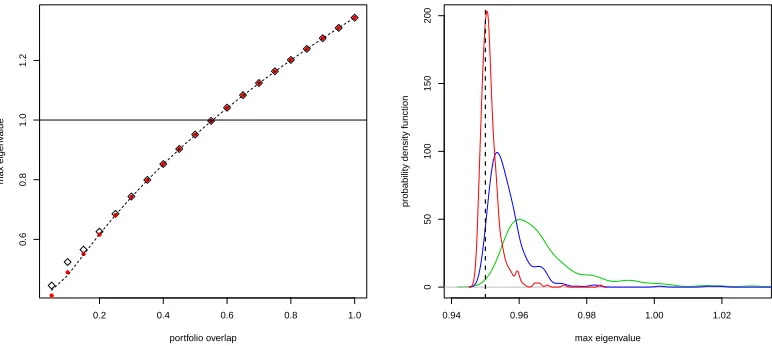
Figure 4: Left panel. Maximum eigenvalue Λmax as a function of the mean fractional overlap

¯

o between two portfolios when N = 1,000. The dashed black line is the result of Eq. 24. Red circles and black diamonds are the mean maximum eigenvalue over 500 simulations

when banks have homogeneous asset size and asset size drawn from lognormal distribution

with µ= 11.7 and σ2 _{= 1.8 (as in Janicki and Prescott (2006)), respectively. Right panel.}

Estimation of the probability density function of the maximum eigenvalue in the case of

lognormal asset size distribution,m = 10, andN = 250 (green), 500 (blue), and 1,000 (red). The vertical dashed line is the theoretical value of Eq. 24.

2.4.2 Numerical simulations and the role of bank size heterogeneity

We investigate numerically the approximations made in the previous calculations considering

the role of bank size heterogeneity and of the number of banks N. For simplicity we will show the results for M = 20 investment assets, α = 1.64, σd = 0.03 σs = 0, and γ = 54.

Similar results are observed for other parameters values.

First we set the number of banks equal toN = 1,000 and we assume that they have all the same asset size. We perform 500 numerical simulations of the matrixWand for each of them

we compute the maximum eigenvalue. We then compare its mean value over the simulations

with the theoretical value (see red circles in the left panel of Figure 4). As a comparison,

we also consider a realistic bank asset size distribution. It is well known that bank size is

the empirical results of Janicki and Prescott (2006) who fitted the asset size of the roughly

10,000 US banks with a lognormal distribution with parameters µ = 11.7 and σ2 = 1.8. Left panel of Figure 4 shows that both in the homogeneous and in the heterogeneous case

the agreement between simulations and the theoretical value is excellent. This fact confirms

that in the largeN limit bank size distribution is irrelevant and the approximations leading to Eq. 24 are very good.

We then consider the role of finite size corrections, investigating the distribution of the

maximum eigenvalue for fixed fractional overlap and variable number of banks N. Specifi-cally, we consider the lognormal distribution of bank size and we fix the value of m = 10. The right panel of Fig. 4 reports the estimation of the probability density function of the

maximum eigenvalue for N = 250,500,1,000. As expected from the convexity argument, form small value ofN the probability density function of the maximum eigenvalue has con-siderable mass above the theoretical (and asymptotic) value of Eq. 24 (vertical dashed line).

Notice however that even for N = 250 the mode of the distribution is only 1% larger than the theoretical value, confirming again that our numerical approximation is very good.

In conclusion this result indicates the asymptotic (in N) nature of our analytical ap-proximation. As suggested above, the finite sample bias is due to the nonlinear and convex

nature of the maximum eigenvalue. In fact, numerical simulations and t-tests confirm that

the mean value ofBij is correctly described by Eq. 21. In any case it is worth noticing that

our numerical simulations indicate that for finite samples, bank size heterogeneity makes the

financial system more unstable as compared to the homogeneous case. In fact, all else being

equal, for finite and smallN the maximum eigenvalue is larger for the heterogenous than for the homogeneous case, making the system closer to the transition between the stationary

and the non-stationary dynamics.

2.5

Properties of risky asset dynamics

Here we give an exact description of the dynamics of investment assets computing in closed

form the variance-covariance matrix of asset returns. In fact, using the average representation

of Eq. 22, we notice that mΨ can be written as

with the scalarb= _{M c}m , identity matrixI, and the column vector of ones ι. Hence, the VAR for the vector of endogenous components in equation (17) can be rewritten as

et = (1−b)A(et−1+εt) +b MAι(¯et−1+ ¯εt) (26)

with matrix A ≡ ¯λ−1

m Γ

−1 _{and scalars ¯e}

t ≡ _M1 PM_k=1ek,t and ¯εt ≡ _M1 PM_k=1εk,t. The scalar ¯et

can be interpreted as the endogenous return of the market portfolio. Thus, the endogenous

component of an individual investment becomes

ei,t = (1−b)ai(ei,t−1 +εi,t) +b M ai(¯et−1+ ¯εt) (27)

with scalar ai =

¯

λ−1

mγi.

Therefore, the process for ei,t can be rewritten as a linear combination of a standard

univariate AR(1) process and a dynamic process depending on the averages of previous period

endogenous components and shocks. In this way,ei,t is a mixture of a perfectly idiosyncratic

process (i.e. uncorrelated with the others investment processes) receiving weight 1−b and a perfectly correlated process with weight b. Being b= _{M c}m , the higher is the value ofm, the higher is the weight given to the perfectly correlated component of mixture and, hence, the

higher the correlations among the endogenous components of the different investments.

Moreover, assuming ai =a ∀i (i.e. all investments have the same liquidity), the process

for ¯et becomes:

¯

et = a(1−b+bM)(¯et−1+ ¯εt)≡φ(¯et−1+ ¯εt) (28)

with φ ≡ a(1− b +bM). Therefore, the dynamics of the average process ¯et is also an

autoregressive of order one; its variance, assuming stationarity ofet, is (see Appendix D)

V( ¯et) =

Λ2_max 1−Λ2

max

V(¯εt) (29)

with V(¯εt) =

σ2_f +σ2

M

.

Finally, defining the distance of the endogenous component of investment i from the average as ∆ei,t ≡ei,t −¯et, we also have that

where ∆εi,t ≡ εi,t−ε¯t. So that the dynamics of the individual distance of the endogenous

component of investment i from the average value ¯et is also an autoregressive process of

order one.

We can then interpret the dynamics of the endogenous components of each individual

investment as an idiosyncratic AR(1) process around a common process for the average value

also following an AR(1) and where the amplitude of the idiosyncratic component is inversely

related to the portfolio diversification. In other words, the dynamics of endogenous returns

can be described as a multivariate “ARs around AR”. When the process is stationary, the

mean market behavior is described by a mean reverting process. In turn, each investment

performs a mean reverting process around the market mean. It can be shown that the time

scale for mean reversion of the market is always larger than the time scale of reversion of

an investment toward the market mean behavior. Moreover, when m increases the time scale of reversion of individual investment declines, which means that investments become

more quickly synchronized with the mean market behavior. Finally, notice that this type of

multivariate “ARs around AR” dynamics is also followed by the endogenous component of

portfolio returns ep_t ≡ 1

m

Pm

k=1ek,t where the number of assets in portfolio is m < M.

Importantly, this representation clearly shows that, as for the exogenous component, also

the variability of the endogenous component of returns can be decomposed into a systematic

component associated with the volatility of ¯etand an idiosyncratic one. Therefore, both the

exogenous and endogenous components contain a diversifiable and undiversifiable source of

risk, so that also the total risk of the investments return is composed of these two type of

risk, σs and σd, as perceived by the financial institutions.

Thanks to this representation we are able to explicitly compute the variance and

covari-ances of the process for the endogenous components ei,t, which are reported in Appendix

(D). It can be shown that a larger leverage increases both the variances and the covariances

of ei,t, while a greater degree of diversification reduces the variances and increases the

co-variances. Both are positively related with correlations. In particular, it can be shown (see

Appendix D) that the correlations among the endogenous returns tend to one as m→M.9

9_{Notice that the endogenous correlations would not tend to one in presence of an additional stochastic}

component in the price impact function (Eq. 15) coming from the exogenous demand of traders not actively

Taking into account the feedback induced by the portfolio rebalancing introduces a new

endogenous component in the variance of the investment asset given by the variance of the

endogenous component

V(ri,t) =V(ei,t) +V(εi,t) (31)

where the exogenous variance V(εi,t) = σ2f +σ2 and the explicit expression for the

endoge-nous variance V(ei,t) is given in Appendix D. This expression shows that the endogenous

component of return leads to an increase of the volatility of an investment above its “bare”

level V(εi,t). This volatility increase is at the end due to the finite liquidity of the

invest-ments and disappears when γ → ∞ and it can therefore be seen as an “illiquidity induced contribution to volatility”.

Analogously, the covariance between the returns of two investments is enhanced by the

contribution coming from the covariance between the endogenous components (see Appendix

D)

Cov(ri,t, rj,t) =Cov(ei,t, ej,t) +σf2. (32)

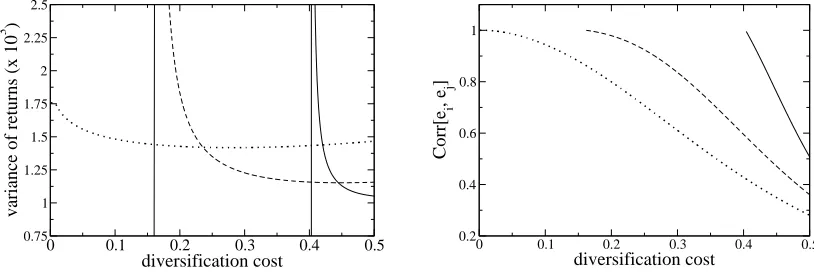
Figure 5 shows the variance of returns and the correlation between the endogenous

com-ponent of returns of two investments as a function of diversification cost c. We see that when cost is high, variance and correlations are low. By decreasing cost, variance of returns

increases as well as correlations. If the market factor is not strong enough, there is a value

of c for which variance diverges, corresponding to the case where the maximum eigenvalue Λmax becomes equal to one. In this limit, correlations become closer and closer to one.

As a consequence the variance of portfolio returns in presence of the rebalancing feedbacks

becomes

V(rp_t) = V(ei,t)

m +

m−1

m Cov(ei,t, ej,t) +σ

2

f +

σ2

m

= V(ep) +σf2 +

σ2

m, (33)

which, as for investment returns, means that the endogenous component (and therefore

the illiquidity of the assets) increases the volatility of portfolio by a illiquidity induced

0 0.1 0.2 0.3 0.4 0.5

diversification cost

0.75 1 1.25 1.5 1.75 2 2.25 2.5

variance of returns (x 10

3 )

0 0.1 0.2 0.3 0.4 0.5

diversification cost

0.2 0.4 0.6 0.8 1

Corr[e

i

, e

j

[image:23.612.93.500.103.241.2]

]

Figure 5: The left panel shows the variance of investment returns, V(ri,t), of Eq. (31) as

a function of the diversification cost c, while the right panel shows the correlation of the endogenous component of returns between two investments, Corr(ei,t, ej,t) as a function of

c (see Fig. 1 for the parameters). The vertical lines in the left panel indicate where the variance of returns diverges and below these values correlations in the right panel are clearly

not defined.

diversification cost c for different values of the ratio σs/σd. It is important to notice that

by reducing diversification cost, the variance of portfolios initially declines. This means that

in this regime, financial innovation makes portfolios less risky and it is therefore beneficial.

However, the variance of the portfolio reaches a minimum for a given value of c and by reducing further the diversification cost, one gets closer and closer to the critical condition

Λmax = 1 and the variance increases without bounds. In this regime, even small variations

of the cost lead to huge increases of the riskiness of the portfolios.

It is also interesting to note that the variance of the observed market portfolio (the one

containing all the M investments with equal weights) is

V(rM_t ) = V(¯e) +σ_f2 + σ

2

M ≡V(¯e) +σ

2

pM =

Λ2 max

1−Λ2 max

σ_p2

M +σ

2

pM

= 1

1−Λ2 max

σ_p2_M (34)

with σ2_pM ≡ σ2_f + σ2

M being the market portfolio return when feedback due to impact is not

can then be termed the “variance multiplier” of the endogenous component. Clearly, for

larger values of the maximum eigenvalue of the VAR process, the variance multiplier will

increase exploding for Λ2

max →1.

0 0.1 0.2 0.3 0.4 0.5

diversification cost

0 0.5 1 1.5 2

variance of portfolios (x 10

3 )

0 0.1 0.2 0.3 0.4 0.5

diversification cost

0.2 0.4 0.6 0.8 1

[image:24.612.92.503.172.313.2]

correlation of portfolios

Figure 6: The left panel shows the variance of portfolios, V(r_tp), of Eq. (33) as a function of the diversification cost c, while the right panel shows their correlation, ρe

p, of Eq. (36) (see

Fig. 1 for the parameters). The vertical lines in the right panel indicate where the variance

of portfolios diverges and below these values correlations in the right panel are clearly not

defined.

Similarly, the covariance between two portfolios containing m assets becomes

Cov(r_h,tp , r_k,tp ) = Cov(ei,t, ej,t) +σf2+m

m M

V(ei,t)−Cov(ei,t, ej,t) +σ2

m2

= V(ei,t)

M +

M −1

M Cov(ei,t, ej,t) +σ

2

f +

σ2

M

= V(¯e) +σ2_f + σ

2

M

= 1

1−Λ2 max

σ_p2_M. (35)

In fact, given the factor structure of ei,t, with the factor being ¯rt= ¯et−1+ ¯εt, the covariance

Cov(ep,t,¯et) is equal to the variance of the factor V(¯e) (as for the exogenous covariance).

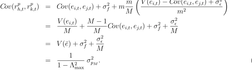
[image:24.612.101.521.499.617.2]

be written as

ρp =

V(¯e) +σ2_f +σ2

M

V(ep) +σf2+ σ2

m

=

V(ep) V(¯e)

V(ep) +

σ_f2+ σ2

m

_σ2

f+ σ2 M

σ2

f+ σ2

m

V(ep) +σ2f + σ2

m

= σ

2

eρe+σε2ρε

σ2

e +σε2

(36)

where σ2

e ≡ V(ep), σε2 ≡ σf2 + σ2

m, ρe ≡

Cov(ep,t,¯et)

V(ep) =

V(¯e)

V(ep), and ρε ≡

σ2

f+ σ2 M

σ2

f+ σ2

m

. That is,

the portfolio correlation in presence of active asset management is a weighted average of the

endogenous correlations betweenep and ¯e, i.e. ρe, and the correlation between the exogenous

shocks, (i.e. ρε), with weights the respective variancesσe2 andσε2. Since both the endogenous

ρe and exogenous ρε correlations tend to one as m → M, also the total correlation of the

portfolio ρp tends to one as m →M.

The right panel of Figure 6 shows the correlation between portfolios as a function of the

diversification cost c. Correlation between portfolios steadily increases by reducing diversi-fication costs essentially because the overlap between portfolios increases. It is important

to notice that the condition of divergence of the variance does not imply a perfect overlap

between portfolio. For example, with the given parameters the transition to infinite variance

and non stationary portfolios occurs at ¯o = 0.34 when σs/σd = 0.3 and at ¯o = 0.21 when

σs/σd = 0. Thus correlation between portfolios can become very close to one even if the

portfolio overlap is relatively small.

2.6

Bank asset dynamics

The dynamics of the rebalanced bank asset A∗_i,t, can be written as

A∗_j,t =λjEj,t =λj Ej,t−1+r

p j,tA

∗

j,t−1

=A∗_j,t−1+λjr p j,tA

∗

j,t−1 (37)

thus, the relative change of the bank j total asset rA

j,t is simply given as

rA_j,t ≡ A ∗

j,t−A

∗

j,t−1

A∗_j,t−1 =λjr

p

j,t. (38)

Therefore, the variance and covariance of the relative change of bank assetsrA

j,tare simply

0 0.1 0.2 0.3 0.4 0.5 diversification cost 0 0.1 0.2 0.3 0.4 0.5 0.6 0.7 0.8

variance of total asset (x 10

6 )

0 0.2 0.4 0.6 0.8 1

portfolio overlap 0 0.1 0.2 0.3 0.4 0.5 0.6 0.7 0.8

variance of total asset (x 10

6 )

Figure 7: Variance of the total asset,PN

j=1r

p

j,t, of the whole banking sector as a function of

the diversification costc(left panel) and of the mean fractional overlap ¯o between portfolios (right panel) (see Fig. 1 for the parameters) The vertical lines indicate where the variance

of total asset diverges.

and

Cov(r_h,tA, r_k,tA) =λhλkCov(rph,t, r p

k,t), (40)

where the expression for V(r_j,tp ) and Cov(rp_h,t, r_k,tp ) are given in equation (33) and (35), re-spectively. The properties of the bank assets dynamics are then dictated by those of the

portfolio (with its exogenous and endogenous components) and further amplified by the

degree of leverage.

We can finally compute the variance of the total asset of the whole banking sector

V

N

X

j=1

r_j,tA

!

'N V rA_j,t+N(N−1)Cov r_h,tA, r_k,tA'Nλ¯2V rp_j,t+N(N−1)¯λ2Cov rp_h,t, rp_k,t

= ¯λ2V

N

X

j=1

rp_j,t

!

(41)

where for simplicity we have assumed that all the banks have the same leverage ¯λ. Moreover

V PN

j=1r

p j,t

is explicitly given in terms of the original variables in Appendix D where it is

also shown that form →M it reduces to

V

N

X

j=1

r_j,tp

!

−−−→

m→M

N2_σ2

pM

1−Λmax

These analytical results allows us to analyze the determinants of the variability of total

asset of the banking sector which governs the expansion and contraction of the supply of

credit and liquidity to financial system.

Figure 7 shows the variance of the total asset of the whole banking sectors as a function

of the diversification cost (left panel) and of the mean fractional overlap between portfolios

(right panel). We observe that the variance of the total asset monotonically increases when

one decreases diversification cost or increases the overlap between portfolios. As one of these

two related variables leads the system close to the critical point, the variance of the total

asset of the banking sector explodes. Moreover, close to the transition point, the variance of

the total asset increases dramatically when one changes slightly the typical overlap between

portfolios.

3

Systemic risk

We now analyze the systemic risk implications of our model first in the static setting without

feedback and then in a setting with the endogenous feedback of investor demands on the

asset dynamics.

3.1

Static analysis

First, as previously shown, when the diversificationm increases, the correlation between the portfolio returns of two financial institutions will increase, with ρp −−−→

m→M 1, which, ceteris

paribus, tends to increase the probability of a systemwide contagion during a crisis event.

Second, given a negative realization of the systematic (exogenous and endogenous)

com-ponent st = ¯et+ft, the portfolio return distribution conditioned on this systematic shock

sshock

t is (considering, for simplicity, a normal distribution for portfolio returns with zero

mean):

rp_i,t|sshock_t ∼N

sshock_t , σ

2

d

m

. (43)

where rp_i,t =Pm

j=1

ri,j,t

m is the portfolio return of bank i at timet.

sshock t is

P Di,t−1 = P

rp_i,t|sshock_t ≤ −α

r

σ2

s +

σ2

d

m

!

(44)

= Φ  

−α

q

σ2

s + σ2

d

m −s shock t

q

σ2

d

m



 −−−−−−−−→

m→M, M→∞ 1 ∀ s

shock

t <−ασs,

where Φ is the standard normal cdf. Therefore, for any negative shock of the systematic

component larger than its VaR, i.e. ασs, the probability of default increases with the degree

of diversification m.

In summary, higher degree of diversification increases both the probability of default of

single institutions (in case of large systematic shocks) and the correlations among them, thus

exposing the economy to a higher level of systemic risk.

3.2

Dynamic analysis

The results of the previous section show that the endogenous return dynamics adds an

additional component to both the variance and covariance of the risky investments. If such

endogenous components were not accounted for in the evaluation of portfolio volatility for

the VaR, obviously, there would be an underestimation of each agent’s risk, leading to an

under capitalization of the banking sector and, hence, to an higher fragility of the system.

Nevertheless, the practice of empirically estimating variances and covariances of risky assets

from past data, automatically considers both the exogenous and endogenous components of

volatility.

However, contrary to the case without endogeneity, the investments variances and

co-variances now depend on the level of diversification and, in particular, the degree of leverage

(through the dynamics of the endogenous component). Therefore, a change, say, in the

de-gree of leverage will cause a structural shift in the future level of variances and covariances

which will not be captured by the empirical estimation on past data.

In particular, in periods when leverage increases, portfolio volatility estimated on

his-torical past data will tend to underestimate future risk (coming from stronger rebalancing

feedback) leading to an increase of systemic risk. On the contrary, in periods of decreasing

realized volatility will tend to be lower than the historical one. Therefore, the results of

our model provide a theoretical support for countercyclical capital requirements as often

advocated in the aftermath of the recent financial crises.

Moreover, it is important to notice that a given negative realization of the exogenous

factor ft, will trigger a sequence of portfolio rebalances causing the price of all risky assets

to decay for several periods. Within our framework, we can explicitly compute the expected

impact on the future return dynamics triggered by a given common shock.

Being et = Φrt (from equation 17), the vector of investment returns also follows a

VAR(1)

rt = et−1+ιft+t =Φrt−1+ιft+t. (45)

The total future impact of the shocks over the next h periods will be given by the h-period cumulative mean return conditioned on the factor shock fshock

t , which is (for h sufficiently

large)

Ert:t+h|ftshock

'(I−Φ)−1ιf_tshock. (46) Hence, the larger the maximum eigenvalue of Φthe larger will be the magnitude and

persis-tence of future adjustments leading to a larger cumulative impact that the financial system

will have to absorb. So the larger the maximum eigenvalue the higher will be the probability

that the system, because of capital or liquidity constraints, will not be able to absorb the

initial shock. This also means that systemic risk is positively related to the magnitude of

the eigenvalues of the matrixΦ.

4

Discussion: Introducing financial innovations

The results on the dynamics of the asset prices can be summarized as follows. When the costs

of diversificationcare high, the degree of diversification i.e. the number of assetmrandomly selected and the degree of leverage are small. Thus the portfolio of the financial institutions

are heterogeneous and little leveraged. Therefore, the endogenous feedbacks, coming from

the amplification of individual demands induced by leverage targeting (as illustrated in the

at the aggregate level between asset values and prices of risky investments will not tend to

arise.

We now discuss the effect of the introduction of financial innovation products (such as

securitization of mortgages or ABS products) that permits to reduce the cost of diversification

c. Despite the simplicity of our framework, the introduction of financial innovation has several important consequences. First, a financial innovation which reduces the cost of

diversification c, by increasing the optimal level of diversification m, reduces the volatility of the portfolio which in turns increase the leverage of the institution. In this way, financial

innovation will tend to increase the degree of leverage in the system. By increasing the

leverage, the individual exposition to the undiversifiable macro factor risk increases; i.e.,

although each individual is more resilient to idiosyncratic shocks, they become more sensitive

to the shocks in the macro factor.

Second, by increasingm, the overlap in the portfolios of the different financial institutions will be larger, increasing the ”similarity” of the portfolio choices among the investors and,

thereby, increasing the correlations among portfolio returns and balance sheet dynamics.

Third, an increase in leverage will heavily affect the dynamics of the risky investments

by increasing both their variances, covariances and correlations, through a strengthening of

the endogenous component.

As a consequence of these effects, individual reactions in terms of asset demands will

be more aggressive (due to higher leverage) and more coordinated (because of the larger

correlation in the profits-losses realizations). This rise in the strength and coordination of

the individual reactions will make more likely to have aggregate feedback in which the rise of

the price of some investments leads to an excess of equity (by the realized capital gains) and,

hence, to an expansion of the balance sheets driving new demands for the asset which pushes

the price up and so on. The very same mechanism will operate also in the opposite direction

during market crisis when the aggregate feedback will aggravate price declines and balance

sheet contractions. When the diversification cost falls below a given threshold (implying

the maximum eigenvalue of the vector return process exceeding one) the aggregate feedback

will produce price and balance sheet dynamics that become explosive (see also Corsi and

[image:31.612.176.432.81.235.2]

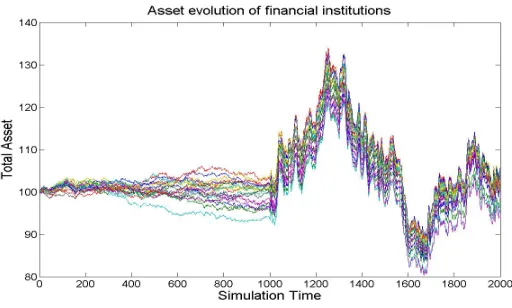
Figure 8: Numerical simulation of the dynamics of individual total asset of financial

insti-tutions before and after a structural break (at simulation time 1000) on the diversification

costs that induces an increase of leverage and diversification. Leverage goes from 10 to 60

and fractional overlap from 0.1 to 0.8 .

These feedbacks could be reinforced even further by endogenizing the dynamics of

finan-cial innovation or, as in Brunnemeier and Pedersen (2008), that of the market liquidity. For

instance, following the intuition of Brunnemeier and Pedersen (2008), the market liquidity

could be assumed to inversely depends on the past realized volatility so that an increase

in the endogenous feedback, by increasing volatility also increase the market impact of the

portfolio rebalancing (through the reduction in market liquidity), thus further reinforcing

the feedback.

Therefore, through these mechanisms reinforcing the endogenous feedback, financial

in-novation can give rise to a steep growth (bubble) and plunge (burst) of market prices and

banking sector total assets. As explained by Adrian and Shin (2010), the total asset of the

banking sector is the relevant variable for the determination of the amount of credit supplied

to the financial and real sector. Hence, an increase in the variability of the total asset of the

banking sector will have major consequences on the availability of funding to the economy

causing the instability to be transmitted from the financial sector to the real one.

To visually illustrate the impact on the dynamics of financial intermediaries total asset

of a shift in the degree of leverage and diversification induced by a reduction in the

sudden increase (at simulation time 1000) in the degree of leverage and diversification (see

Figure 8). Going from a low level of leverage and diversification to a high level we observe:

(i) a dramatic increase in the correlation and amplitude of the changes in the total asset

of individual financial institutions, and (ii) a sudden shift in the total banking sector assets

(i.e. simply the sum of all the individual bank total assets), which will imply going from an

approximately constant supply of credit to a regime with wide swings in the credit supply.

5

Conclusions

In this paper we investigate the determinants of the balance sheet dynamics of financial

intermediaries by modeling the dynamic interaction between asset prices and bank behavior

induced by regulatory constraints and multi-round portafoglio rebalances. Standard capital

requirements, in the form of Value–at–Risk (VaR) constraints, together with the level of

diversification costs (related to the availability of derivatives products), determine bank

decisions on diversification and leverage which, in turns, strongly affect the dynamics of

traded assets through the bank strategies of portfolio rebalances in presence of a finite asset

liquidity. We show how changes in the constraints of the bank portfolio optimization (such

as changes in the prevailing cost of diversification or changes in the micro-prudential policies)

endogenously drive the dynamics of bank balance sheets, asset prices, and systemic risk.

The analytical results obtained by applying our simple framework are manifolds: (i) a

reduction of diversification costs, by increasing the level of diversification and hence relaxing

the VaR constraint, allows the financial institutions to increase the optimal leverage; (ii)

it also increases the degree of overlap, and thereby correlation, between the portfolios of

financial institutions; (iii) even in absence of feedback effects, higher degree of diversification

increases both the probability of default of single institutions (in case of large systematic

shocks) and the correlations among them, thus exposing the economy to a higher level of

systemic risk; (iv) the higher overlap induced by a reduction in diversification costs increases

both the variance and correlation of the investment demands of financial institutions

re-balancing their portfolios; (v) the dynamic interaction between investment prices and bank

max-imum eigenvalue depends on the degree of leverage and on the average illiquidity of the

assets; (vi) higher diversification, by increasing the strength and coordination of individual

feedbacks, can lead to dynamic instability of the system; (vii) the VAR process can be

rep-resented as a combination of many idiosyncratic AR processes around a single common AR

process of the average values; (viii) the endogenous feedback introduces an additional

com-ponent to the variance, covariance and correlation of both the individual investment assets

and the bank portfolios; (ix) both the variance and correlation of individual investments

monotonically increase with a reduction in the diversification costs; (x) a simple variance

multiplier exists for the variance of the observed market portfolio. (xi) the relation between

the variance of the portfolio and diversification costs is non-monotonic as it initially declines

with costs while then rapidly increases when the reduction of diversification costs makes

the system approaching its critical point causing the variance to explode; (xii) the effects

of the endogenous feedback make historical estimation of variances and covariances to be

overestimated during periods of increasing leverage and underestimated during periods of

deleveraging, thus providing a rationale for the adoption of countercyclical capital

require-ments; (xiii) in presence of endogenous feedbacks, a negative realization of the systematic

component will trigger a sequence of portfolio rebalances which will amplify, over time, its

initial impact; (xiv) the variability of total asset of the banking sector, which governs the

expansion and contraction of the supply of credit and liquidity to financial system, is highly

sensitive to variation in the costs of diversification.

Acknowledgements

Authors acknowledge Piero Mazzarisi for useful discussions. The research leading to these

results has received funding from the European Union, Seventh Framework Programme

FP7/2007-2013 under grant agreement n◦ CRISIS-ICT-2011-288501.

References

Adrian, T. and Boyarchenko, N. (2012). Intermediary leverage cycles and financial stability.