CES technology and business cycle fluctuations

City, University of London Institutional Repository

Citation

:

This is the accepted version of the paper.

This version of the publication may differ from the final published

version.

Permanent repository link:

Link to published version

:

Copyright and reuse:

City Research Online aims to make research

outputs of City, University of London available to a wider audience.

Copyright and Moral Rights remain with the author(s) and/or copyright

holders. URLs from City Research Online may be freely distributed and

linked to.

City Research Online: http://openaccess.city.ac.uk/ publications@city.ac.uk

CES Technology and Business Cycle Fluctuations

Cristiano Cantore University of Surrey

Paul Levine University of Surrey

Joseph Pearlman City University London

Bo Yang

Xi’an Jiaotong - Liverpool University University of Surrey

September 1, 2015

Abstract

We contribute to an emerging literature that brings the constant elasticity of substi-tution (CES) specification of the production function into the analysis of business cycle fluctuations. Using US data, we estimate by Bayesian-Maximum-Likelihood methods a standard medium-sized DSGE model with a CES rather than Cobb-Douglas (CD) technology. We estimate a elasticity of substitution between capital and labour well below unity at 0.15-0.18. In a marginal likelihood race CES decisively beats the CD production and this is matched by its ability to fit the data better in terms of second moments. We show that this result is mainly driven by the implied fluctuations of factor shares under the CES specification. The CES model performance is further im-proved when the estimation is carried out under an imperfect information assumption. Hence the main message for DSGE models is that we should dismiss once and for all the use of CD for business cycle analysis.

JEL Classification: C11, C52, D24, E32.

Keywords: CES production function, DSGE model, Bayesion estimation, Imperfect information

∗

1

Introduction

This paper extends a standard medium-sized DSGE model developed by Christianoet al.

(2005) and Smets and Wouters (2007) to allow for a richer and more data coherent

spec-ification of the production side of the economy. The idea is to enrich what has become

the workhorse DSGE model by relaxing the usual Cobb-Douglas production assumption

in favour of a more general CES function. This then allows for cyclical variations in factor

shares, the estimation of the capital/labour elasticity of substitution and biased technical

change.

The CES production function has been used extensively in many area of economics

since the middle of the previous century (Solow (1956) and Arrowet al.(1961)). Thanks to

La Grandville (1989), who introduced the concept ofnormalization, it has been extensively

used in growth theory.1 Factor substitution and the bias in technical change feature an

important role in many other areas of economics2 _{but, until recently have been largely}

disregarded in business cycle analysis. On the empirical side Le´on-Ledesmaet al. (2010)

show that normalization improves empirical identification.3

The concepts of biased technical change and imperfect factor substitutability between

factors of production have been introduced in business cycle analysis by Cantore et al.

(2014b). They show that the introduction of a normalized CES production function into

an otherwise standard Real Business Cycle (RBC) and/or New Keynesian (NK) DSGE

model significantly changes the response of hours worked to a technology shock in both

settings and that such response might change as well within each model depending on the

parameters related to the production process. They also show how the introduction of

biased technical change and imperfect substitutability allow movements in factor shares

which appear to fluctuate at business cycle frequencies in the data but are theoretically

1_{La Grandville (1989) showed that it was possible to obtain a perpetual growth in income per-capita,}

even without any technical progress. See Cantore and Levine (2012) for a recent perspective on normal-ization.

2

The value of the substitution elasticity has been linked to differences in international factor returns and convergence (e.g., Klump and Preissler (2000), Mankiw (1995)); movements in income shares (Blanchard (1997), Caballero and Hammour (1998), Jones (2003)); the effectiveness of employment creation policies (Rowthorn (1999)), etc. The nature of technical change, on the other hand, matters for characterizing the welfare consequences of new technologies (Marquetti (2003)); labour-market inequality and skills premia (Acemoglu (2002)); the evolution of factor income shares (Kennedy (1964), Acemoglu (2003)) etc.

3_{They show that using a normalized approach permits to overcome the ’impossibility theorem’ stated}

constant under the Cobb-Douglas specification.4 Indeed there is mounting evidence in the

literature5 that whilst constant factor shares might be a good approximation for growth

models where the time span considered is very long, at business cycle frequencies those

shares are not constant. This is clearly shown in Figure 1 for the US data used to estimate

our model.

84Q1 85Q1 86Q1 87Q1 88Q1 89Q1 90Q1 91Q1 92Q1 93Q1 94Q1 95Q1 96Q1 97Q1 98Q1 99Q1 00Q1 01Q1 02Q1 03Q1 04Q1 05Q1 06Q1 07Q1 08Q2 71%

72% 73% 74% 75% 76%

Labour Share (84:1−08:2)

Figure 1: US Labour Share (Source: U.S. Bureau of labour Statistics)

There is also increasing interest in reconciling the apparent long run constancy of factor

shares with the short-run fluctuations. Le´on-Ledesma and Satchi (2011) approach is based

on the choice of technologies by firms in terms of their capital intensity and results in a

new class of production functions that produces short-run capital-labour complementarity

but yields a long-run unit elasticity of substitution.6 Koh and Santaeulalia-Llopis (2014)

use a non-constant elasticity of substitution production function allowing the elasticity to

vary over time in the short run while keeping the Cobb-Douglas assumption in the long

run. They estimate this elasticity in a perfectly competitive setting and find that the

elasticity is countercyclical and shocks are on average biased towards labour.7

4

Furthermore Cantoreet al.(2012) test empirically the model(s) developed by Cantoreet al.(2014b) using rolling-windows Bayesian techniques in order to check if the documented time-varying relation be-tween hours worked, productivity and output (see Fernald (2007) and Gal´ı and Gambetti (2009) among others) can be explained using the threshold rule.

5_{See for example Blanchard (1997), Jones (2003, 2005), McAdam and Willman (2013) and R´ıos-Rull}

and Santaeul´alia-Llopis (2010).

6_{See also Le´on-Ledesma and Satchi (2015) for an approach based on the concept of a technology frontier.}

7

In the DSGE literature however, most models continue to use the Cobb-Douglas

as-sumption even if the empirical evidence provided through the years has ruled out the

possibility of unitary elasticity of substitution (see among others Antr`as (2004), Klump

et al. (2007), Chirinko (2008) and Le´on-Ledesma et al. (2010)). In this paper we show

that the introduction of a CES production function in a medium-scale DSGE model in

the spirit of Christianoet al. (2005) and Smets and Wouters (2007) makes it possible to

exploit the movements of factor shares we observe in the data to improve significantly

the performance of the model. To the best of our knowledge, we are the first to compare

the empirical implications of CD and CES production functions in a medium scale DSGE

context using Bayesian-Maximum-Likelihood comparison.8

The main results of our paper are first: in terms of model posterior probabilities,

im-pulse responses, second moments and autocorrelations, the assumption of a CES

technol-ogy significantly improves the model fit. Second, this finding is robust to the information

assumption assumed for private agents in the model. Indeed allowing the latter to have

the same (imperfect) information as the econometrician (namely the data) further

im-proves the fit compared with the standard assumption that they have perfect information

of all state variables including the shock processes. Third, using US data, we estimate by

Bayesian-Maximum-Likelihood (BML) the elasticity of substitution between capital and

labour to be 0.15-0.18, a value broadly in line with the literature using other methods of

estimation.9

solved only in isolation and with the introduction of frictions and/or non-competitive settings. The four puzzles being: i) The low (or even negative) correlation between real wage and output; ii) the vanishing procyclicality of labour productivity (see Gal´ı and van Rens (2014)); iii) the negative correlations of labour share and output and its components including its overshooting response of labour share to productivity; iv) the negative hours-productivity correlation.

8_{Choi and R´ıos-Rull (2009) and Koh and Santaeulalia-Llopis (2014) also present a comparison of CD}

vs CES. Choi and R´ıos-Rull (2009) use a calibrated version of their model with CES with a specific value of the elasticity of substitution (0.75), that turns out to be quite high compared to recent estimates, and show that the implied responses of the economy to a productivity shock are very similar, apart from the labour share response that shows a mild overshooting. Koh and Santaeulalia-Llopis (2014) instead compare NCES (non-constant elasticity of substitution) with constant CES and CD production. Our comparison here differs from theirs on three dimensions. First they perform a non-linear estimation of their model while here we are estimating a first order approximation of a DSGE model using perturbation methods. For this reason we are able to compute posteriors probabilities. Second we are not allowing the elasticity of substitution between capital and labour to vary over time. Third we are comparing the production functions in a medium scale DSGE model with nominal and real frictions allowing for a larger set of shocks while their comparison of their model against non-competitive settings is done conditional only to productivity shocks.

9

As we show later in the paper the first result is mainly driven by the implied fluctuations

of factor shares under the CES specification. Although the main focus of the paper is not

to match labour share moments and business cycle behaviour, this paper is related to

a fast growing literature on the cyclical behaviour of the labour share which we briefly

review below in order to put our model and results in context.

Although cyclical properties of factor shares have been understudied for many years,

scholars have reached a wide consensus regarding two business cycle characteristics of the

labour share. Labour share is countercyclical (but with a low correlation) on impact and

it overshoots following productivity innovations.10 This overshooting behaviour has been

presented by R´ıos-Rull and Santaeul´alia-Llopis (2010) who find that, conditional on

pro-ductivity shocks, the labour share in U.S. is negatively correlated with contemporaneous

output but positively with lagged output (5 quarters or more).

To explain the contercyclicality some authors have focused on market rigidities that

prevent prices and volumes to adjust perfectly and rapidly to shocks. Gomme and

Green-wood (1995) and Boldrin and Horvath (1995) introduce labour and insurance contracts

into the market which enable risk sharing between workers and firms.11

Choi and R´ıos-Rull (2009) introduce a RBC model with search and matching frictions

and a non-competitive labour market, where wages and hours are not determined by

their marginal products but by a bargaining process. Wages then exceed the marginal

product of labour, while employment remains fixed due to the search frictions. This

leads to a sluggish, countercyclical behaviour of the share.12 Bentolila and Saint-Paul

(2003) argue that changes in the product market markups, occurring due to imperfect

competition, may cause a cyclical movement of the labour share as they fluctuate over the

business cycle. A procyclical markup in the product market may cause countercyclical

10_{Hansen and Prescott (2005) discuss macroeconomic dynamics in the light of countercyclical labour}

shares in the US between 1954 and 1993. The European Commission (2007) showed detailed business cycle behaviour of the labour share for European countries confirming countercyclicality for all countries except Germany. Choi and R´ıos-Rull (2009) and R´ıos-Rull and Santaeul´alia-Llopis (2010) find that the labour share in the short run is relatively volatile, countercyclical, highly persistent, lagging output and overshoots the initial loss after a positive technology shock.

11

Similar to the idea of introducing sticky wages into a model through implicit contracts by Boldrin and Horvath (1995) and Gomme and Greenwood (1995) suggests that only a subset of workers and firms bargain over wages at each point in time so that wages cannot be adjusted immediately after an increase in productivity. After such an increase prices and productivity go up while there is only a sluggish adjustment of aggregates wages.

12

shifts in the labour share. Shao and Silos (2014) introduce costly entry of firms in a model

with frictional labour markets and find that the key to replicate factor share dynamics

is to have a weak correlation between the real interest rate and output. Colciago and

Rossi (2015) show that Nash bargaining delivers a countercyclical labour share while

countercyclical mark-ups deliver the overshooting response. What all these papers have in

common is that there are frictions or adjustments in the short run that create endogenous

fluctuations in the labour share while maintaining the CD assumption in production.13

Koh and Santaeulalia-Llopis (2014) instead present a competitive market framework, using

a flexible production function (non-constant CES in the short run and CD in the long run)

and are able to replicate and match the cyclical behaviour of the labour share and various

labour market variables. From this literature it emerges that we are able to match second

moments of the labour share in different settings. We have a wide set of different competing

models explaining the same behaviour in terms of second moments. Here in this paper

we provide an additional one which does not require an extensive modification of the

workhorse medium scale DSGE used extensively in the literature and by policy-makers.

We follow the conclusion of Choi and R´ıos-Rull (2009) and Cantore et al. (2014b) that,

in order to match the cyclical behaviour of the labour share, we should focus on a more

general specification of the production side of the economy, rather than on non-competitive

factor markets.

Finally there is also a growing literature looking at the long-run behaviour of the labour

share in the U.S. pointing towards an observed decline in its trend since the 70s (see Piketty

and Zucman (2014) and Neiman and Karabarbounis (2014) amongst others.) This implies

that, in order to match empirical phenomena, the macroeconomic literature should move

away from linear and stationary models, as in the one presented here, and develop models

of the U.S. economy featuring a non-stationary labour share. However there remains a

substantial degree of uncertainty and disagreement in the literature regarding the

long-run decline in the labour share. Muck et al. (2015) show that the consequences of the

ambiguity in the empirical definition of the labour share do not matter much for the

short run, but do affect its long-run trend. Their preferred measure, amongst the various

examined, does show a decline from the 70s but also a substantial increase before that.

For this reason they suggest that we should focus not only on the decline in recent years

but extend the sample in order to explain this observed hump shaped response. Bridgman

(2014) focuses on the differences between gross and net labour share. He shows that once

we take into account items that do not add to capital, depreciation and production taxes

net labour share is within historical averages and does not show a significant decline as

we observe in gross measures. Finally Kohet al.(2015) show that labour share computed

in an economy with only structures and equipment capital is indeed stationary, which

actually is, the case of the economy considered here.

The rest of the paper is organised as follows. Section 2 summarise the model with

particular attention paid to the normalization of the CES production function. Section 3

sets out the BML estimation of the model. Section 4 examines the ability of the models

to capture the main characteristics of the actual data as described by second moments,

discusses identification and sensitivity issues and presents the models implied response of

labour share conditional on productivity shocks. Section 5 concludes the paper.14

2

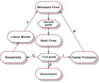
Summary of the Model

Here we summarise the Smets and Wouters (2007) augmented model (SW) with a

whole-sale and a retail sector, Calvo prices and wages, CES production function, adjustment

costs of investment and variable capital utilization.15 Figure 2 illustrates the model

struc-ture. The novel feature is the introduction of a CES production function in the wholesale

sector, instead of the usual Cobb-Douglas form. This generalization then allows for the

identification of both labour-augmenting and capital-augmenting technology shocks. As in

Smets and Wouters (2007) we use a household utility function compatible with a balance

growth path in the steady state, but we adopt a more standard functional form used in

the RBC literature. However we do not adopt Kimball aggregators for final output and

composite labour.16 Again as in their paper we introduce a monopolistic trade-union that

14_{The online Appendix available here presents the full derivation of the model, the estimation result}

together with figures for prior and posterior distribution of the parameters for the baseline model estimated with asymmetric information and identification and sensitivity analysis details for the labour market and input elasticity of substitution parameters.

15_{For the full model derivation and equilibrium conditions see the Section A in the online Appendix.}

16

allows households to supply homogeneous labour. Then as long as preference shocks are

symmetric, households are identical in equilibrium and the complete market assumption

is no longer required for aggregation. The supply-side of the economy consists of

com-petitive retail sector producing final output and a monopolistically comcom-petitive wholesale

sector producing differentiated goods using the usual inputs of capital and work effort.

Households consume a bundle of differentiated commodities, supply labour and capital to

the production sector, save and own the monopolistically competitive firms in the goods

sector. Capital producers provide the capital inputs into the wholesale sector.17

The sequencing of decisions is as follows:18

1. Each household supplies homogeneous labour at a price Wh,t to a trade-union.

Households choose their consumption, savings and labour supply given aggregate

consumption (determining external habit). In equilibrium all household decisions

are identical.

2. Capital producing firms convert final output into new capital which is sold on to

intermediate firms.19

3. A monopolistic trade-union differentiates the labour and sells typeNt(j) at a price

Wt(j) to a labour packer in a sequence of Calvo staggered wage contracts. In

equilib-rium all households make identical choices of total consumption, savings, investment

and labour supply.

4. The competitive labour packer forms a composite labour service according to a

constant returns CES technologyNt=

R1

0 Nt(j)

(ζ−1)/ζ_djζ/(ζ−1) _{and sells onto the}

17

There are other differences with Smets and Wouters (2007): (i) Our price and wage mark-up shocks follow an AR(1) process instead of the ARMA process chosen by SW; (ii) in SW the government spending shock is assumed to follow an autoregressive process which is also affected by the productivity shock; (iii) we have a preference shock instead of the risk-premium shock. Chariet al.(2009) criticise the risk premium shock arguing that it has little interpretation and is unlikely to be invariant to monetary policy. We prefer our somewhat simpler set-up and we expect none of the differences to affect the main focus of the paper which is on the comparison between CD and CES production functions.

18_{Sequencing matters for the monopolistic trade-unions and intermediate firms who anticipate and}

ex-ploit the downward-sloping demand for labour and goods respectively. Different set-ups with identical equilibria are common in the literature. Monopolistic prices can be transferred to the retail sector. When it comes to introducing financial frictions, for example, as in Gertler and Karadi (2011) the introduction of separate capital producers as in our set-up is convenient, but not essential in the SW model without such frictions.

19

intermediate firm.

5. Each intermediate monopolistic firm f using composite labour and capital rented

from capital producers to produce a differentiated intermediate good which is sold

onto the final goods firm at price Pt(f) in a sequence of Calvo staggered price

contracts.

6. Competitive final goods firms use a continuum of intermediate goods according

to another constant returns CES technology to produce aggregate output Yt =

R1

0 Yt(f)(µ

−1)/µ_dfµ/(µ−1)_.

We then solve the model by backward induction starting with the production of final

goods as we show in Section A of the online Appendix. Below we discuss in details the

CES production and itsnormalization, the choice of utility function and list the exogenous

shocks of the model.

Capital Producers

Households

Retail Firms

Intermed. goods

Wholesale Firms

Government

Labour Market

G

I C

K L

Final goods

2.1 The Normalized CES Production Function

The production function is assumed to be CES as in Cantore et al. (2014b) which nests

Cobb-Douglas as a special case and admits the possibility of neutral and non-neutral

technical change. Here we adopt the ‘re- parametrization’ procedure described in Cantore

and Levine (2012) in order to normalize the CES production function:

Yt =

h

αk(ZKtUtKt)ψ+αn(ZNtNt)ψ i_ψ1

−F;ψ6= 0 &αk+αN 6= 1

= (ZKtUtKt)αk(ZNtNt)αn−F;ψ→0 & αk+αN = 1 (1)

where Yt, Kt, Nt and Ut are wholesale output, capital and labour inputs and variable

capital utilisation respectively at time tand ψ is the substitution parameter andαk and

αn are sometimes referred as distribution parameters. The terms ZKt and ZNt capture

capital-augmenting and labour-augmenting technical progress respectively.20 Calling σ

the elasticity of substitution between capital and labour,21withσ ∈(0,+∞) andψ= σ−_σ1

then ψ ∈ (−∞,1). When σ = 0 ⇒ ψ = −∞ we have the Leontief case, whilst when

σ= 1⇒ψ= 0 (1) collapses to the usual Cobb-Douglas case.

From the outset a comment on dimensions would be useful. Technology parameters

are not measures of efficiency as they depend on the units of output and inputs (i.e., are

not dimensionless22) and the problem of normalization arises because unless ψ → 0, αn

andαk in (1) are not shares and in fact are not dimensionless.

20

We are in the case of Hicks neutrality ifZKt =ZNt >0, Solow neutrality ifZKt>0 andZNt= 0

and Harrod neutrality in the case ofZKt= 0 andZNt>0.

21_{The elasticity of substitution for the case of perfect competition, where all the product is used to}

remunerate factor of productions, is defined as the elasticity of the capital/labour ratio with respect to the wage/capital rental ratio. Then callingW the wage andR+δthe rental rate of capital we can define the elasticity as follows:

σ= d

K L

L K

d_RW_+δR_W+δ.

See La Grandville (2009) for a more detailed discussion. 22

For example for the Cobb-Douglas production function in the steady state, Y = Kα(AN)1−α, by dimensional homogeneity, the dimensions ofA are (output per period)1−1α _{/ ((person hours per period}

)×(machine hours per period )1−αα_{). For some this poses a fundamental problem with the notion of a}

Marginal products of labour and capital are respectively

FN,t =

Yt

Nt "

αn(ZNtNt)ψ

αkZKtUtKtψ+αn(ZNtNt)ψ #

=αnZNtψ

Yt

Nt 1−ψ

(2)

FK,t =

Yt

Kt "

αkZKtUtKtψ

αkZKtUtKtψ+αn(ZNtNt)ψ #

=αk(UtZKt)ψ

Yt

Kt 1−ψ

(3)

The equilibrium of real variables depends on parameters defining the RBC core of the

model%,σc,δ,ψ,αk andαn, and those defining the NK features. Of the former,%,ψand

σc are dimensionless,δ depends on the unit of time, but unlessψ= 0 and the technology

is Cobb-Douglas,αkandαndepend on the units chosen for factor inputs, namely machine

units per period and labour units per period. To see this rewrite the wholesale firm’s foc23

in terms of factor shares

WtNt

P_tWYt

= αnZNtψ

Yt

Nt −ψ

(4)

(Rt−1 +δ)Kt

P_tWYt

= αk(UtZKt)ψ

Yt

Kt −ψ

(5)

whereP_tW ≡ M CtPt is the price of wholesale output, Wt is the nominal wage and Rt is

the real interest rate. Then we have

WtNt

(Rt+δ)

= αn

αk

ZKtUtKt

ZNtNt −ψ

(6)

Thus αn (αk) can be interpreted as the share of labour (capital) iff ψ = 0 and the

pro-duction function is Cobb-Douglas. Otherwise the dimensions of αk and αn depend on

those forZKtUtKt

ZNtNt

ψ

which could be for example, (effective machine hours per effective

person hours)ψ. In our aggregate production functions we choose to avoid specifying unit

of capital, labour and output.24 _{It is impossible to interpret and therefore to calibrate or}

estimate these ‘share’ parameters.

There are two ways to resolve this problem; ‘re-parameterize’ the dimensional

pa-rameters αk and αn so that they are expressed in terms of dimensionless ones, with all

23

Equations A.6 and A.7 in the Online Appendix. 24

Unlike the physical sciences where particular units are explicitly chosen so dimension-dependent pa-rameters pose no problems. For example the fundamental constants such as the speed of light is expressed in terms of metres per second; Newtons constant of gravitation has units cubic metres per (kilogram×

parameters to be estimated or calibrated (see Cantore and Levine (2012)), or ‘normalize’

the production function in terms of deviations from a steady state. We consider these in

turn.

2.1.1 Re-parametrization of αn and αk

On the balanced-growth path (BGP) consumption, output, investment, capital stock, the

real wage and government spending are growing at a common growth rate g driven by

exogenous labour-augmenting technical changeZNt+1 = (1 +g)ZNt, but labour inputN

is constant.25 As is well-known a BGP requires either Cobb-Douglas technology or that

technical change must be driven solely by the labour-augmenting variety (see, for example,

Jones (2005)). ThenZKt=ZK must also be constant along the BGP.

On the BGP let capital share and wage shares in the wholesale sector beα and 1−α

respectively. Then using (4) and (5) we obtain ourre-parameterization ofαn andαk:

αk=α

¯

Yt

ZKU¯tK¯t ψ

(7)

αn= (1−α) ¯

Yt

ZNtN ψ

(8)

Note that αk =α and αn = 1−α at ψ = 0, the Cobb-Douglas case.26 This completes

the stationarized equilibrium defined in terms of dimensionless RBC core parameters %,

σc, ψ,α and δ which depends on the unit of time, plus NK parameters. In (7) and (8)

dimensional parameters are expressed in terms of other endogenous variablesYW,N and

K which themselves are functions of θ ≡ [σ, ψ, α, δ,· · ·]. Therefore αn = αn(θ), and

αk=αk(θ) which expresses why we refer to this procedure as reparameterization.

There is one more normalization issue: the choice of units at some point say t = 0

on the steady state BGP. We use for simplicity ¯Y0 = ZN0 = ZK = 127 but, as it

is straightforward to show that having expressed the model in terms of dimensionless

parameters re-parameterization makes the steady state ratios of the endogenous variables

of the model independent of this choice.

25

If output, consumption etc are defined in per capita terms thenN can be considers as the proportion of the available time at work and is therefore both stationary and dimensionless.

26

And as argued before ifα∈(0,1)αk+αn= 1 iffψ= 0.

27

By assuming ¯Y0= 1 we implicitely assume ¯Y0W = ¯

Y0

2.1.2 The Production Function in Deviation Form

This simply bypasses the need to retain αk and αn and writes the dynamic production

function in deviation form about its steady state as

Yt

¯

Yt

=

αk(ZKtUtKt)ψ +αn(ZNtNt)ψ

αk(ZKU¯tK¯t)ψ+αn(ZNtN)ψ _ψ1 =    αk

ZKtUtKt

ZKU¯tK¯t

ψ

αk+αn

ZNtN

ZKU¯tK¯t

ψ +

αn

ZNtNt

ZNtNt

ψ

αk

ZKU¯tK¯t

ZNtN

ψ

+αn 

 

1

ψ

Then from (7) and (8) we can write this simply as

Yt

¯

Yt

=

"

(1−α)

ZKtUtKt

ZKU¯tK¯t ψ

+α

ZNtNt

¯

ZNtN ψ#_ψ1

(9)

as in Cantore et al. (2014b). The steady-state normalization now consists of ZN0 =

¯

Y0 =ZK = 128 and is characterized entirely by fixed shares of consumption, investment

and government spending and by labour supply as a proportion of available time, all

dimensionless quantities apart from the unit of time.

Using either of these two approaches, as showed by Cantore and Levine (2012), the

steady state ratios of the endogenous variables and the dynamics of the model are not

affected by the starting values of output and the two source of shocks ( ¯Y0, ZN0, ZK)

which only represent choice of units. Crucially, this implies also that changingσ does not

change our steady state ratios and factor shares, impulse response functions are directly

comparable, and parameter values are consistent with their economic interpretation.

2.2 Utility Function

The household utility function is of a Cobb-Douglas-CRRA form chosen to be compatible

with a balanced-growth steady state and allowing for external habit-formation:

Ut =

eBt((Ct−χCt−1)(1−%)(1−Nt)%)1−σc−1

1−σc

(10)

UC,t = eBt(1−%)(Ct−χCt−1)(1−%)(1−σc)−1((1−Nt)%(1−σc)) (11)

UN,t = −eBt%(Ct−χCt−1)(1−%)(1−σc)(1−Nt)%(1−σc)−1 (12)

28

where Ct is aggregate consumption, χ is the habit formation parameter, σc measures

relative risk aversion, % is the inverse of the Frisch elasticity of labour supply and eBt is

a preference shock.

2.3 Shock Processes

As we show in the Online Appendix the model has a total of seven AR(1) exogenous

shocks29 plus the iid shock to the monetary policy rule. The seven autoregressive shocks

are in order: capital-augmenting, labour-augmenting, investment specific, preference,

gov-ernment spending, price and wage mark-up.

3

Estimation

We estimate the linearized version of the model around zero steady state inflation by

Bayesian methods using DYNARE. We use the same observable set as in Smets and

Wouters (2007) in first difference at quarterly frequency but extend the sample length to

the second quarter of 2008, before the outbreak of the 2008 crisis. Namely, these observable

variables are the log differences of real GDP, real consumption, real investment and real

wage, log hours worked, the log difference of the GDP deflator and the federal funds rate.

As in Smets and Wouters (2007), hours worked are derived from the index of average hours

for the non-farm business sector and we divide hourly compensation from the same sector

by the GDP price deflator to obtain the real wage. All series are seasonally adjusted. All

data are taken from the FRED Database available through the Federal Reserve Bank of

St.Louis and the US Bureau of Labour Statistics. The sample period is 1984:1-2008:2.

The corresponding measurement equations for the 7 observables are:30

29

Expressed in log deviation forms: logXt−logX =ρX(logXt−1−logX) +X,t. Where ρX and εX

will be the autoregressive parameter and the standard deviation of shock X respectively. 30

                

D(logGDPt)∗100

D(logCON St)∗100

D(logIN Vt)∗100

D(logW AGEt)∗100

log(GDP DEFt/GDP DEFt−1)∗100

F EDF U N DSt/4

HOU RSt

                 =                   log Yt Yt −log Yt−1

Yt−1

+ ctrend log Ct Ct −log Ct−1

Ct−1

+ ctrend log It It −log It−1

It−1

+ ctrend

log

Wt/Pt

Wt/Pt

−log

Wt−1/Pt−1

Wt−1/Pt−1

+ ctrend

log Πt

Π

+ conspie

logRn,t

Rn

+ consrn

log Nt

N + conslab                  

The first four potentially non-stationary observables (output Yt, consumption Ct,

in-vestment It and the real wage Wt/Pt) are taken in first differences, while gross inflation

Πt, the gross nominal interest rate Rn,t, and hours worked Nt, are used in levels. We

introduce a common trend in the first-differenced variables and a specific one for inflation,

nominal interest rate and hours worked.

3.1 Bayesian Methodology

Bayesian estimation entails obtaining the posterior distribution of the model’s parameters,

say θ, conditional on the data. Using the Bayes’ theorem, the posterior distribution is

obtained as:

p(θ|YT) = L(Y

T_|θ)p(θ) R

L(YT_|θ)p(θ)dθ (13)

where p(θ) denotes the prior density of the parameter vector θ, L(YT|θ) is the

like-lihood of the sample YT with T observations (evaluated with the Kalman filter) and

R

L(YT|θ)p(θ)dθ is the marginal likelihood. Since there is no closed form analytical

ex-pression for the posterior, this must be simulated.

One of the main advantages of adopting a Bayesian approach is that it facilitates a

formal comparison of different models through their posterior marginal likelihoods,

com-puted using the Geweke (1999) modified harmonic-mean estimator. For a given model

vectorθ,

L YT|mi

=

Z

Θ

L YT|θ, mi

p(θ|mi)dθ (14)

wherepi(θ|mi) is the prior density for model mi, and L YT|mi

is the data density for

model mi given parameter vector θ. To compare models (say, mi and mj) we calculate

the posterior odds ratio which is the ratio of their posterior model probabilities (or Bayes

Factor when the prior odds ratio, p(mi)

p(mj), is set to unity):

P Oi,j =

p(mi|YT)

p(mj|YT)

= L(Y

T_|m

i)p(mi)

L(YT_|m

j)p(mj)

(15)

BFi,j =

L(YT|m_i)

L(YT_|m j)

= exp(LL(Y

T_|m i))

exp(LL(YT_|m j))

(16)

in terms of the log-likelihood. Components (15) and (16) provide a framework for

com-paring alternative and potentially misspecified models based on their marginal likelihood.

Such comparisons are important in the assessment of rival models, as the model which

at-tains the highest odds outperforms its rivals and is therefore favoured. Given Bayes factors,

we can easily compute the model probabilitiesp1, p2,···, pnfornmodels. SincePni=1pi = 1

we have that _p1

1 =

Pn

i=2BFi,1, from which p1 is obtained. Thenpi =p1BF(i,1) gives the

remaining model probabilities.

3.2 Likelihood Comparison of Models

We compare four different model specifications in order to see if the introduction of factor

substitutability and/or the biased technical change improves the fit of the estimation.

In the first row of Table 1 we present the likelihood density of the model with the CD

production function where only the labour-augmenting technology shock is present. In

the second row we introduce the CES and calibrate the elasticity of substitution to 0.4

(CES0), following the literature as in Cantore et al. (2014b) and Klump et al. (2012),

and introduce the capital-augmenting shock whilst in rows 3 (CES1) and 4 (CES2) we

estimateσ in a model with and without the latter shock. Strictly speaking a meaningful

likelihood comparison that provides information about σ is only possible between row 1

and 3 (where we can compare like for like without adding a further exogenous shock).

CD counterpart with a posterior probability of 100%. This suggests that incorporating a

CES production function offers substantial improvements in terms of the model fitness to

the data in the US economy. The differences in log marginal likelihood are substantial.

For example, the log marginal likelihood difference between the first two specifications is

12.47 corresponding to a posterior Bayes Factor of 2.6041e+05. As suggested by Kass and

Raftery (1995), the posterior Bayes Factor needs to be at least e3 ≈20 for there to be a

positive evidence favouring one model over the other.

Model σ Technology shocks Log data density Difference with CD

CD 1 ZN -544.60 0

CES0 calibrated=0.4 ZK & ZN -532.13 12.47

CES1 estimated=0.15 ZN -528.50 16.10

CES2 estimated=0.15 ZK & ZN -528.31 16.29

Table 1: Marginal Likelihood Comparison Between CD and CES Specifications

3.3 Estimation under the Standard Information Assumptions

In this section we make the standard information assumption in solving rational

expec-tations models that economic agents have perfect information about the realizations of

current shocks and other relevant macroeconomic variables, alongside their knowledge of

the model, parameter values and the policy rule, whereas the econometrician uses only

ob-servable data. In effect the private sector has more information than the econometrician,

so we refer to this case asasymmetric information (AI).

The joint posterior distribution of the estimated parameters is obtained in two steps.

First, the posterior mode and the Hessian matrix are obtained via standard numerical

op-timization routines. The Hessian matrix is then used in the Metropolis-Hastings (MH)

al-gorithm to generate a sample from the posterior distribution. Two parallel chains are used

in the Monte-Carlo Markov Chain Metropolis-Hastings (MCMC-MH) algorithm. Thus,

250,000 random draws (though the first 30% ‘burn-in’ observations are discarded) from the

posterior density are obtained via the MCMC-MH algorithm, with the variance-covariance

matrix of the perturbation term in the algorithm being adjusted in order to obtain

rea-sonable acceptance rates (between 20%-30%).

Estimation results from posteriors maximization are presented in Section D of the

parameters whereas we used a loose prior for the elasticity of substitution between capital

and labour in order to see if the data are informative about the value of this parameter.

A few structural parameters are kept fixed or calibrated in accordance with the usual

practice in the literature of choosing them to target steady state values of some observed

variables (see Table 2).31

Calibrated parameter Symbol Value

Discount factor β 0.99

Depreciation rate δ 0.025

Growth rate g ₄δ

Substitution elasticity of goods ζ 7 Substitution elasticity of labour µ 7 Variable capital utilization γ1 1_β +δ−1

Fixed cost F_Y 1−M C = 1_ζ = 0.1429 Preference parameter % _1+N(c1−N

y(1−χ)/α−1)

Implied steady state relationship

Government expenditure-output ratio gy 0.2

Investment-output ratio iy ₍₁(1_/β−₋α₁₊)δ_δ)

Consumption-output ratio cy 1−gy−iy

Table 2: Calibrated Parameters

First we focus on the posterior estimates obtained using the most general CES model,

CES2. As shown in Tables D.1 and D.2 in the online Appendix, the point estimates under

the CES assumption are tight and plausible. In particular, focusing on the parameters

characterizing the degree of price stickiness and the existence of real rigidities, we find that

the price indexation parameters are estimated to be smaller than assumed in the prior

distribution (in line with those reported by Smets and Wouters (2007)). The estimates of

the indexation parametersγpandγwimply that inflation is intrinsically not very persistent

in the CES model specifications. The posterior mean estimates for the Calvo parameters,

ξpandξw, imply an average price contract duration of around 2.31 quarters and an average

wage contract duration of around 1.84 quarters, respectively. These results are in general

consistent with the findings from empirical works on the DSGE modelling in the US

economy. It is interesting to note that the risk-aversion parameter (σc) is estimated to be

less than assumed in the prior distribution, indicating that the inter-temporal elasticity

31

of substitution (proportional to 1/σc) is estimated to be about 0.86 in the US, which is

plausible as suggested in much of RBC literature. As expected, the policy rule estimates

imply a fairly strong response (απ) to expected inflation by the US Fed Reserve and the

degree of interest rate smoothing (αr) is fairly strong.

Figure E.1 in the online Appendix plots the prior and posterior distributions for the

above CES model. The location and the shape of the posterior distributions are largely

independent of the priors we have selected since priors are broadly less informative. Most

of the posterior distributions are roughly symmetric implying that the mean and median

coincide. According to Figure E.1, there is little information in the data for some

pa-rameters where prior and posterior overlap.32 Perhaps the most notable finding comes

from the estimation of the parameter σ - our key parameter in the CES setting. As a

result of assuming a very diffuse prior with large standard deviation, we find that the data

is very informative about this parameter (as clearly shown in the figure, curves do not

overlap each other and are very different) and the point estimate ofσin Table D.1 is close

to the plausible values. This further provides strong evidence to support the empirical

importance of the CES assumption.

We now turn to the comparisons between parameter estimates under CD and CES

specifications. Parameter posteriors that are quantitatively different33from the estimation

using a Cobb-Douglas specification are underlined in Tables D.1 and D.2.

Starting with the parameters related to the exogenous shocks (Table D.1) we notice

that the estimated standard deviations of the newly introduced capital-augmenting

tech-nology shock is very small but, probably because of its introduction, the standard deviation

of the investment specific shock reduces significantly (from 4.16 in the CD specification

to 3.06 in the CES case).34 We also notice that the estimated standard deviations of the

mark-up shocks are lower under the CES specification and the standard deviation of the

preference shock is slightly higher. The autoregressive parameters of the exogenous shocks

are not affected significantly by the CES choice.

Posterior estimation of the investment adjustment costs parameter (φX_{) reduces by}

0.75 when we estimate the model under CES showing once again how introducing

factor-32

In particular parametersρZK,σc,γp,γwandαare weakly identified.

33

Difference in posteriors up to 0.05 were not considered quantitatively relevant here. 34

biased technical change affects significantly the estimation of ‘investment-related’

param-eters. The parameters of the utility function also appear to be affected by the choice of

the production function (σc reduces by 0.94 and χ reduces by around 0.21). Regarding

the parameters associated with sticky prices and wages both the probabilities of no

price-adjustment (ξp) and no wage-adjustment (ξw) change significantly, decreasing from 0.77

to 0.57 and 0.60 to 0.46, respectively. Monetary policy weights (except the weight on

inflation which increases slightly), real and nominal trends estimations are not affected by

the introduction of factor substitutability and biased technical change.

3.4 Estimation under Symmetric Imperfect Information

In our estimation procedure up to now we have followed the standard practice of assuming

agents forming rational expectations have perfect information of all states, include shock

processes, whereas the econometrician only observes the data variables. This we refer to

as the asymmetric information (AI) assumption. Based on the methodology developed

in Levine et al. (2012), we now relax this extreme information assumptions and instead

assume that both private agents and the econometrician have thesame imperfect

informa-tion (II) and both use the Kalman Filter, the former to form expectations of unobserved

state variables and the latter to calculate the likelihood in the Bayesian estimation.

Al-though perfect information on idiosyncratic shocks may be available to economic agents, it

is implausible to assume that they have full information on economy-wide shocks.

Further-more, as shown in Levineet al.(2012), as long as the number of shocks exceed the number

of observables (as is the case in our set-up), the solutions under II and AI differ and the

latter provides an alternative source of endogenous persistence that offers the potential

for capturing the dynamics observed in the data. We therefore empirically address these

alternative information assumptions to assess whether parameter estimates are consistent

across them and which of these choices leads to a better model fit.

We provide the estimation results from posteriors maximization for Model CES2, the

‘best’ model in Table 1, under II. The following table provides a formal Bayesian

compar-ison between CES2 under AI and II respectively.35

35

Model σ Technology shocks Log data density Difference with CD CES2AI estimated=0.15 ZK & ZN -528.31 16.29

CES2II estimated=0.18 ZK & ZN -524.59 20.01

Table 3: Marginal Likelihood Comparison Between AI and II

It is clear from Table 3 that the assumption of imperfect information leads to a better

fit as implied by the marginal likelihoods. Recalling Kass and Raftery (1995), a Bayes

factor of 10-100 or a log data density range of [2.30, 4.61] is ‘strong to very strong

evi-dence’. For our Model CES2, there is ‘strong’ evidence in favour of the II assumption.

The differences in log data density or the posterior odds ratio are substantive when

com-paring models assuming both CES and II with the model with CD. For example, the log

marginal likelihood difference between Model CES2 under II and Model CD is 20.01. In

order to choose the former over Model CD, we need a prior probability over Model CD

4.9004e+08(= e20.01_{) times larger than our prior probability over Model CES2 under II}

and this factor is decisive.

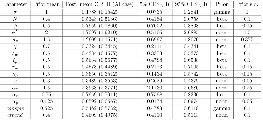
Parameter Prior mean Post. mean CES II (AI case) 5% CES (II) 95% CES (II) Prior Prior s.d.

ρZN 0.5 0.9470 (0.9443) 0.9059 0.9932 beta 0.2

ρZK 0.5 0.4980 (0.4441) 0.1887 0.8325 beta 0.2

ρG 0.5 0.9613 (0.9631) 0.9418 0.9782 beta 0.2

ρZI 0.5 0.7961 (0.7429) 0.6817 0.9117 beta 0.2

ρP 0.5 0.9672 (0.9744) 0.9399 0.9955 beta 0.2

ρW 0.5 0.9750 (0.9656) 0.9565 0.9938 beta 0.2

ρB 0.5 0.8728 (0.9311) 0.7977 0.9503 beta 0.2

εZN 0.1 0.6905 (0.6833) 0.5944 0.7793 invg 2.0

εZK 0.1 0.0804 (0.0744) 0.0240 0.1492 invg 2.0

εG 0.5 1.9947 (1.9904) 1.7650 2.2374 invg 2.0

εZI 0.1 2.8668 (3.0647) 1.4762 4.2147 invg 2.0

εP 0.1 0.3771 (0.3756) 0.3093 0.4370 invg 2.0

εW 0.1 0.9781 (0.9482) 0.8328 1.1282 invg 2.0

εM 0.1 0.1604 (0.1579) 0.1371 0.1832 invg 2.0

εB 0.1 1.0863 (1.4997) 0.7681 1.3876 invg 2.0

Table 4: Posterior Results for the Exogenous Shocks (II vs AI)

We now turn to the comparisons between parameter estimates under AI and II (Tables

4 and 5). Overall, the parameter estimates are plausible and reasonably robust across

information specifications, despite the fact that the II alternative leads to a better model

fit based on the corresponding posterior marginal likelihood. It is interesting to note that

assuming II for the private sector reinforces the evidence that theZK and ZI shocks are

Parameter Prior mean Post. mean CES II (AI case) 5% CES (II) 95% CES (II) Prior Prior s.d.

σ 1 0.1788 (0.1542) 0.0735 0.2841 gamma 1

N 0.4 0.5343 (0.5136) 0.4184 0.6758 beta 0.1

φ 0.5 0.7959 (0.7860) 0.7052 0.8838 beta 0.15

φX _{2 1.7097 (1.9210) 0.5106 2.6885 norm 1.5}

σc 1.5 1.2609 (1.1571) 0.6997 1.8070 norm 0.375

χ 0.7 0.3324 (0.3445) 0.2111 0.4341 beta 0.1

ξw 0.5 0.4384 (0.4577) 0.3373 0.5373 beta 0.1

ξp 0.5 0.5634 (0.5677) 0.4788 0.6538 beta 0.1

γw 0.5 0.4578 (0.4489) 0.2123 0.7005 beta 0.15

γp 0.5 0.3656 (0.3512) 0.1434 0.5742 beta 0.15

α 0.3 0.3489 (0.3553) 0.2629 0.4379 norm 0.05

απ 1.5 2.3968 (2.3771) 2.1130 2.6680 norm 0.25

αr 0.75 0.7959 (0.7911) 0.7598 0.8336 beta 0.1

αy 0.125 0.0592 (0.0667) 0.0174 0.0974 norm 0.05

conspie 0.625 0.5462 (0.5732) 0.4783 0.6118 gamma 0.1

ctrend 0.4 0.4609 (0.4975) 0.4110 0.5113 norm 0.1

Table 5: Posteriors Results for Model Parameters (II vs AI)

deviations of the capital-augmenting technology shock (ZK) is slightly larger and as a

result the standard deviation of the investment specific shock (ZI) further reduces (from

3.06 under AI to 2.87 in the II case). This again confirms our finding early that when

ZK is absent ZI is capturing “capital-biased” technological progress and the degree of

which depends on whether the shocks are observed or not by the private sector. The other

significant change in estimates from AI to II is from the investment adjustment costs

parameter (φX) and this shows how assuming II helps provide evidence that introducing

factor-biased technical change affects significantly the estimation of ‘investment-related’

parameters. Our model comparison analysis contains one important result suggesting

that a combination of incorporating CES and with information set II offers a decisive

improvement in terms of the model fit, dominates the standard CD model with a very

large log-likelihood difference of around 20.

4

Model Validation

After having shown the model estimates and the assessment of relative model fit to its

other rivals with different restrictions, we use them to investigate a number of key

macroe-conomic issues in the US. The model favoured in the space of competing models may still

be poor (potentially misspecified) in capturing the important dynamics in the data. To

nec-essary to compare the model’s implied characteristics with those of the actual data. In

this section, we address the following questions: (i) can the models capture the underlying

characteristics of the actual data? (ii) Are the parameters, especially the labour market

and production ones, identified? Are the results robust to calibration and estimation

as-sumptions? (iii) are the models able to reproduce the overshooting property of the labour

share conditional to productivity innovations?

4.1 Standard Moment Criteria

Summary statistics such as first and second moments have been standard as means of

validating models in the literature on DSGE models, especially in the RBC tradition. As

the Bayes factors (or posterior model odds) are used to assess the relative fit amongst

a number of competing models, the question of comparing the moments is whether the

models correctly predict population moments, such as the variables’ volatility or their

correlation, i.e. to assess the absolute fit of a model to macroeconomic data.

To assess the contributions of assuming different specifications of production function

in our estimated models, we compute some selected second moments and present the

re-sults in this section. Table 6 presents the (unconditional) second moments implied by the

above estimations and compares with those in the actual data. In terms of the standard

deviations, all models generate relatively high volatility (standard deviations) compared

to the actual data (except for the interest rate and the CD production assumes constant

labour share). Overall, the estimated models are able to reproduce broadly acceptable

volatility for the main variables of the DSGE model and all model variants can successful

replicate the stylized fact in the business cycle research that investment is more volatile

than output whereas consumption is less volatile. In line with the Bayesian model

com-parison, the models with CES technology fit the data better in terms of implied volatility,

getting closer to the data in this dimension (we highlight the ‘best’ model (performance)

in bold). Note that all our CES models clearly outperform the CD model in capturing

the volatilities of all variables (except for hours) and CES2 with II does extremely well

at matching the investment and real wage volatilities in the data. Furthermore by not

imposing a constant labour share as in the CD model CES2 with II generates the

likelihood comparison, the differences in generating the moments between the CES

specifi-cation with only the shock ZN and the CES with both ZK and ZN shocks are qualitatively

very small.

Standard Deviation

Output Consumption Investment Wage Inflation Interest rate Hours Labour share

Data 0.58 0.53 1.74 0.66 0.24 0.61 2.47 2.07

(0.50,0.69) (0.46,0.62) (1.54,2.01) (0.57,0.82) (0.21,0.27) (0.55,0.70) (2.09,2.94) (1.81,2.37) CD 0.78(0.05) 0.69(0.05) 1.87(0.20) 0.99(0.09) 0.43(0.07) 0.44(0.07) 2.84(0.84) 0 CES1 0.69(0.05) 0.66(0.03) 1.82(0.16) 0.73(0.05) 0.43(0.08) 0.50(0.08) 5.76(1.47) 3.83(0.84) CES2 0.69(0.05) 0.66(0.03) 1.81(0.16) 0.73(0.05) 0.43(0.08) 0.50(0.09) 5.79(1.48) 3.85(0.89) CES2II 0.69(0.05) 0.66(0.03) 1.80(0.16) 0.72(0.05) 0.36(0.08) 0.50(0.09) 4.09(1.48) 2.59(0.89)

Cross-correlation with Output

Data 1.00 0.61 0.64 -0.11 -0.12 0.22 -0.25 -0.05

( - ) (0.46,0.74) (0.47,0.75) (-0.40,0.10) (-0.31,0.10) (0.02,0.39) (-0.48,-0.00) (-0.26,0.16) CD 1.00 0.76(0.06) 0.57(0.06) 0.59(0.09) -0.11(0.09) -0.37(0.05) 0.11(0.02) -CES1 1.00 0.43(0.07) 0.63(0.04) 0.13(0.11) -0.08(0.06) -0.11(0.05) 0.03(0.02) -0.23(0.04) CES2 1.00 0.43(0.07) 0.63(0.04) 0.13(0.11) -0.07(0.07) -0.11(0.05) 0.03(0.02) -0.23(0.04) CES2II 1.00 0.47(0.07) 0.63(0.04) 0.15(0.11) -0.06(0.07) -0.15(0.05) 0.06(0.02) -0.28(0.04)

Autocorrelation (Order=1)

Data 0.28 0.17 0.56 0.17 0.54 0.96 0.93 0.90

(0.19,0.37) (0.07,0.27) (0.46,0.66) (0.07,0.26) (0.45,0.64) (0.87,1.00) (0.84,1.00) (0.81,1.00) CD 0.37(0.05) 0.42(0.06) 0.58(0.06) 0.50(0.05) 0.69(0.05) 0.89(0.02) 0.93(0.03) -CES1 0.29(0.04) 0.32(0.05) 0.61(0.04) 0.38(0.05) 0.79(0.07) 0.94(0.02) 0.99(0.01) 0.99(0.01) CES2 0.29(0.04) 0.31(0.05) 0.61(0.04) 0.37(0.05) 0.79(0.08) 0.94(0.02) 0.99(0.01) 0.99(0.01) CES2II 0.28(0.04) 0.33(0.05) 0.63(0.04) 0.36(0.05) 0.66(0.08) 0.91(0.02) 0.98(0.01) 0.98(0.01)

Table 6: Second Moments of the Model Variants (at the Posterior Means)†

Note. † Numbers in bold represent the closest fit to the data.

For the empirical moments computed from the dataset the bootstrapped 95% confidence bounds based on the sample estimates are presented in parentheses; For the moments generated by the estimated models the standard errors based on the model simulation are shown in parentheses. We sample randomly 1000 of the retained parameter draws from the posterior distribution of the estimated models. For each sample the models are solved and simulated to give the finite

sampling distribution of the second moments in which we construct the standard errors.

Table 6 also reports the cross-correlations of the seven observable variables plus labour

share vis-a-vis output. All models perform successfully in generating the positive

con-temporaneous correlations of consumption and investment observed in the data. All CES

models fit the output-investment correlation with the data very well. The highlighted

numbers in this category together with the evidence above show that the feature of CES

in the model is particularly important in characterizing the investment dynamics.

How-ever, as evidence from the implied volatilities confirms, the main shortcoming of all the

models, including the preferred one, is the difficulty at replicating the cross-correlations of

data. This is not a very surprising result because, for DSGE models with even more

fric-tions and distorfric-tions in the labour market, those moments are usually difficult to match.

One promising way of matching those correlations is given by Koh and Santaeulalia-Llopis

(2014). They allow the elasticity of substitution between capital and labour to be time

varying and find that its countercyclicality helps in matching the cross correlations of wage

and labour productivity with output. All models also fail to predict the positive

correla-tion between output and interest rate and CES models have problems in replicating the

negative contemporaneous cross-relation between inflation and output. This is consistent

with the work of Smets and Wouters (2003) as they find that the implied cross-correlations

with the interest rate and inflation are not fully satisfactory. Nevertheless, the results in

general show that, in the models where the CES specification is present, cross-correlations

of endogenous variables are generally closer to those in the actual data.36 It is the

empir-ical relevance of the CES feature that helps to explain the better overall fit as found in

the likelihood race.

To summarise, overall BML based methods suggest that the ability of the model’s

second moments to fit those of the data generally match the outcome of the likelihood

race. The CES model assuming the II set delivers a better fit to the actual data for most

of the second moment features in Table 6. However, as noted above, the differences in the

second moments of the two competing CES variants are very small.

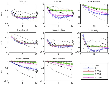
4.2 Autocorrelation Functions

We have so far considered autocorrelation only up to order 1. To further illustrate how

the estimated models capture the data statistics and persistence in particular, we now

plot the autocorrelations up to order 10 of the actual data and those of the endogenous

variables generated by the model variants in Figure 3.

The CES models all stay within the 95% uncertainty bands and II CES2 model

per-forms a little better than its AI counterpart. The inflation autocorrelations generated by

CD model lie outside the 95% uncertainty bands. Of particular interest is that, when

assuming CES production, the implied autocorrelograms fit very well the observed

au-36

0 5 10 −0.5 0 0.5 1 ACF Output

0 5 10

−0.5 0 0.5 1 ACF Inflation

0 5 10

−0.5 0 0.5 1 ACF Interest rate

0 5 10

−1 −0.5 0 0.5 1 ACF Investment

0 5 10

−0.5 0 0.5 1 ACF Consumption

0 5 10

−0.2 0 0.2 0.4 0.6 ACF Real wage

0 5 10

−0.5 0 0.5 1 ACF Hours worked data CD CES1 CES2 CES2II

0 5 10

−0.5 0 0.5 1 ACF Labour share

Figure 3: Autocorrelations of Observables in the Data and in the Estimated Modelsz

Note. z _{The approximate 95% confidence bands are constructed using the large-lag standard}

errors (See Anderson (1976)).

tocorrelation of inflation, interest rate, investment and real wage, whilst the CD model

generates much less sluggishness and is less able to match the autocorrelation of inflation,

interest rate and real wage observed in the data from the second lag onwards. Overall

we find that, with nominal price stickiness in the models and highly correlated estimated

price markup shocks, inflation persistence can be captured closely in DSGE models when

CES production is assumed.

When it comes to output, all models perform well in matching the observed output

persistence. However, the hours is more autocorrelated in all models than in the data,

but now the model with the CD feature gets much closer to the data for higher order

autocorrelations. All models match reasonably well the autocorrelations of investment

and consumption. To summarise, the results for higher order autocorrelations for the

are better at capturing the main features of the US data, strengthening the argument that

the assumption of CES helps to improve the model fit to data.

4.3 Identification and Sensitivity Analysis

In order to verify the robustness of the results discussed above, we conduct a series of

experiments and checks on the variants of our CES model. In this section we address the

following two questions: (a) How well identified are those parameters related to the labour

market? (b) How sensitive are the results to the value of the capital/labour elasticity of

substitution? We focus then on: the labour elasticity of substitution that enters in the

wage mark-up µ, wage indexation γw, the Calvo coefficient for wage contracts ξw and

the elasticity of substitution, σ. Initially, we carry out a formal check on the inherent

identifiability of the models structure by running a series of tests described in Iskrev (2010a,

2010b). The procedure in Iskrev (2010b) reveals whether there are identification problems,

stemming from the Jacobian matrix of the mapping from the structure parameters to the

moments of the observation. We carry out the local identification check for the whole

set of the estimated parameters in the model at a chosen central tendency measure at the

defined priors. For the ‘global’ check we conduct the Monte Carlo exploration in the entire

prior space by drawing 10000 sets of parameters to evaluate the Jacobian matrix. These

tests reveal that the Jacobian matrix is of full rank everywhere in the space of the prior

range so all these parameters, including our key elasticity of substitution parameter for

the CES productionσ, are well-identified within a theoretically admissible range defined

by the prior distribution.

We then examine more carefully the identification ofγw,ξw,µ andσ at the means of

the prior and posterior distributions and using the prior uncertainty. To completely rule

out a flat likelihood and account for the possibility of weak identification we quantify the

identification strength and check collinearity between the effects of different parameters

on the likelihood (following the sensitivity measure in Iskrev (2010a)). If there exists

an exact linear dependence between a pair and among all possible combinations their

effects on the moments are not distinct and the violation of this condition must indicate

a flat likelihood and lack of identification. Table F.1 in the online Appendix reports the

in affecting the likelihood through their effects on the moments of the observed variables.

ξw, in the prior space or estimated, has the strongest effects and µ is the weakest on the

moments among them. The collinearity results suggest, that there is no linear dependence

between the columns of the Jacobian matrix (non-identification) across the prior points

and the estimated parameters in our various CES models.

Alternatively, model CES2 is then tested by using diffuse priors forµ,γwandξw, based

on the normal distribution with one standard deviation for µ and the open unit interval

with [0.229,0.733] at the 95% probability level for γw and ξw, reflecting our uncertainty

about the values of these parameters. We find that the posteriors are relatively insensitive

to the change.37

As an additional check on our results, we experiment with different priors for σ and

different parameterizations forγw andξw, and we re-estimate the preferred model CES2II.

As already noted, our estimate ofσ is almost at the lower bound of the previous available

estimates in the literature38 so this part of the exercise focuses on checking whether our

results with CES are sensitive to an alternative set of parameterization and/or higher

degree ofσ. Our complete findings are available upon request, and the remainder of this

section restricts itself to key results.

Model CES2II is re-estimated imposing the Smets and Wouters (2007) estimates of

the wage dynamics parametersγw andξw. We find that the posteriors are sensitive to this

change and the log marginal likelihood deteriorates significantly (-537.63), suggesting that

it fails to compete with all previous models. In Section 3.2 we have already compared a

model withσcalibrated to 0.4 and found that the model performance is in fact worse than

the cases whenσ is estimated. In this section we carry out a further test by re-estimating

the model under II, using this calibration, combined with the Smets and Wouters (2007)

estimates. It shows that calibrating the model with higher degrees of σ leads to a worse

model fit.

It is also interesting to know whether the dynamics of the variables are altered and

the moments of which variables are most strongly affected by the parameter changes. To

find out, we compute model-generated unconditional moments which are reported in Table

F.3 in the online Appendix. Both models using the alternative parameterization show an

37_{The full set of results are in Table F.2 of the online Appendix.}

38

improvement in matching the standard deviation of hours worked at the expense of other

moments – the ability of matching almost all other moments in this dimension is distorted,

generating much volatility than the data. The performance is even worse whenσ = 0.4 is

imposed and in this case the volatility of labour share is under-estimated, lying well below

the lower bound of the confidence bands.39 Overall, the results we show in this section

suggest that the parameter identification, estimation precision of the NK labour market

and the estimated CES elasticity in our CES model should not be a reason for concern

given the data.

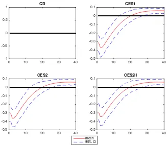
4.4 Productivity and the Labour Share

In this section we present the performance of the model(s) focusing on the conditional

correlation of the labour share to productivity. We want to check if our model is able

to replicate the overshooting behaviour of the labour share following productivity shocks.

As showed by R´ıos-Rull and Santaeul´alia-Llopis (2010), following productivity shocks, the

labour share in U.S. is negatively correlated with contemporaneous output but positively

with lagged output (after 5 quarters or more). First we show that all of our models with

the CES specification can reproduce an impulse response of the labour share to the labour

augmenting shock that is negative on impact and turns positive afterwards.40 Figure 4

shows the impulse response of the labour share in the four models conditional on a ZN

shock simulated at the posterior mean.41 _{Even if this proves that, in principle, our CES}

models can match the overshooting behaviour of the labour share there are two of points

to raise here. First R´ıos-Rull and Santaeul´alia-Llopis (2010) and Koh and

Santaeulalia-Llopis (2014) have shown, in their SVAR analysis, that the change in sign of the impulse

response of the labour share tends to happen in between quarter 4 and quarter 10.42

39

For completeness, we also check the sensitivity in the conditional moments by comparing the estimated impulse responses. The results are not reported here.

40

This property of the CES production function was shown already by Choi and R´ıos-Rull (2009) and Cantoreet al. (2014b). In the ECB working paper version of Cantoreet al. (2014b), as opposed to the published version that has a unit root in the labour augmenting shock, it is evident how both RBC and NK models with CES can reproduce such impulse response of the labour share conditional on a labour augmenting shock. This has to do with the sensitivity in the response of hours to the elasticity of substitution showed by Cantoreet al.(2014a).

41

Results are qualitatively similar using the posterior mode and median and are available under request. 42