Numerical Modelling Techniques to Predict Rotor
Imbalance Problems in Tidal Stream Turbines
Stephanie Ordonez-Sanchez
#1, Kate Porter
#2, Robert Ellis
*1, Carwyn Frost
$1, Matthew Allmark
*2, Thomas
Nevalainen
#3, Tim O’Doherty
*3, Cameron Johnstone
#4#Energy Systems Research Unit, University of Strathclyde Glasgow, G1 1XJ, United Kingdom
* School of Engineering, Cardiff University
Cardiff, CF24 3AA, United Kingdom
*1[email protected] *2[email protected]
$School of Natural and Built Environment, Queen’s University Belfast
Belfast, BT9 5AG, United Kingdom
Abstract—Load fluctuations caused by the unsteady nature of tidal
streams can have severe impacts on turbine components. As seen in the wind industry, turbine blades can become misaligned due to a fault in the pitch mechanism or blade deformations arising over time. These misalignments will represent a loss of power capture and perhaps even premature failure of the components if not detected in time. Computational fluid dynamic (CFD) techniques can be used to predict the performance of a turbine with a misaligned blade. However, these numerical modelling techniques quickly become computationally expensive when modelling realistic, time-varying conditions. Blade Element Momentum Theory (BEMT) offers a quicker and simpler approach, although with several limitations. In this paper BEMT is adapted to predict the performance of a three bladed tidal turbine with one or two blades offset from the optimum pitch setting. This approach is compared with a CFD model to study the effectiveness of both methods to predict power and thrust when a rotor blade has an offset. The simulations were undertaken at three flow speeds (0.9, 1.0 and 1.1 m/s). Both numerical models are compared to experimental data that was obtained at a flume tank in similar flow conditions. The results showed that both BEMT and CFD are able to predict power coefficients when there is a small offset of one rotor blade. However, the predictions were poorer when two blades had two different offsets at the same time.
Keywords— Blade Element Momentum Theory;
Computational Fluid Dynamics; Blade Offset; Rotor Imbalance; Numerical Modelling, Tidal Stream Turbine
I. INTRODUCTION
The development of tidal stream technology is progressing rapidly. One example of this is the Meygen project which seeks to deploy up to 398 MW of tidal turbine capacity by 2020 [1]. One of the key challenges for this technology relates to the unsteady nature of the marine currents which can have serious effects on the turbine performance, durability and structural integrity. These effects can be similar or even more significant than those affecting similar technology in the wind energy industry.
Major faults that occur in wind turbines are often associated with the gearbox and blades. The unsteady loading from the variation in wind speed can give rise to a blade offset or
misalignment of one or more blades. These blade offsets can also be a pre-existing problem if the hub mechanism to set the pitch is not accurate or deforms with time. Having a blade offset or misalignment will compromise the performance of the turbine [2]. For example, the latest news released by Atlantis Resources informed that a component of the pitching mechanism of one of the turbines should be replaced due to its exposure to a long idle cycle [3].
To date, methods to detect blade misalignment have been developed mainly for wind turbines, e.g. [2] and [4]. More recently, [5] developed a methodology to detect different failure types in tidal stream turbines (TSTs) using transient analysis on the torque signals in both the time and frequency domains. The experimental work undertaken by [5] consisted of simulating a rotor imbalance problem by misaligning one or two blades to a different pitch setting than the optimum.
Although experimental work allows investigation of complex fluid-structure interactions in the field of tidal energy, this research method is rather expensive. As a consequence the number of tests is limited, and the experiments must be carefully planned to make effective use of testing time.
An alternative solution to experimental research is the use of analytical and numerical modelling. Compared to laboratory tests, simulations are a cheaper solution. Moreover, when using simulations, there is the flexibility of isolating or modifying certain parameters from the studied case.
each section are derived in terms of the induction factors using the known two-dimensional aerodynamic coefficients for the blade geometry. These two sets of equations are then combined to solve for the unknown induction factors and forces to obtain the performance characteristics of the turbine under ‘steady’ flow conditions [6].
BEMT can provide an adequate solution to model the performance of horizontal turbines, but the method is limited in certain respects. The classic BEMT does not take into account the tip and hub losses and is limited to low-medium angles of attack. However, modifications to the basic model can be made by applying correction factors to account for these limitations, as done by [6]. Researchers have also altered the classic model to incorporate additional aspects such as yaw angle (e.g. [7]), and inflow turbulence [8].
CFD is another technique that is widely used in the field of marine energy. CFD is a more complex method compared to BEMT and is based on the Navier-Stokes equations. The method has been used to explore various aspects of the field such as wake characterisation of single turbines and arrays [9]-[10], loading on turbine components [11] and the effects of flow directionality [12], to name a few. Compared to BEMT, CFD can be used to compute complex dynamic simulations. However, there is a compromise between the level of complexity and the computational time required to solve the simulation.
Several studies have compared the performance of a tidal turbine using BEMT and CFD. Johnson et al. [13] presented a direct comparison of the performance of a cross flow turbine using BEMT and CFD (ANSYS CFX). The study showed that CFD predicts marginally higher coefficients of power, thrust and torque than BEMT. Lawson et al. [14] undertook a similar study using BEMT and CFD (STAR CCM) but this time focusing on horizontal axis tidal turbines. Again it was shown that the torque was only slightly higher when computed with CFD. Moreover, the analysis carried out by [15] showed that CFD could predict higher, lower or precise power coefficients, compared to BEMT, depending on the tip speed ratio (TSR). Therefore, these studies demonstrate that the performance of a TST can be calculated to a comparable level of accuracy with both BEMT and CFD models under simple conditions.
All the CFD simulations mentioned above shared some similarities between the conditions used in their models. The work done by [13]-[15] used k-omega turbulence models in the simulations. [14] and [15] used no slip conditions on the turbine surfaces. It was identified that the main discrepancy between models was the grid generation. Even though both of them used unstructured grids, [15] used a combination of elements by setting subdomains in the simulation while [14] did a study to understand the implications of using different grid resolutions. [14] found out that a coarser computational grid resulted in lower values of torque compared to those obtained with high resolution grids.
The aim of this paper is to determine if the effects of a blade offset can also be modelled successfully with BEMT, thereby providing a simpler method for predicting blade performance in these conditions compared to running a CFD model. The
work developed in BEMT was based on a simplistic approach to account for blade offsets in a tidal turbine rotor where the loads computed for different blade pitch settings are combined proportionally to calculate the overall performance of the turbine with one or two blades offset from the optimum. The results of the simulations are then compared to CFD simulations and the power coefficients obtained from experimental data to assess the quality of both numerical tools.
II. METHODOLOGY
This section describes the numerical and experimental techniques employed in this study to quantify the performance of a scaled three bladed horizontal axis turbine of 0.5 m diameter. The blade cross-section was modelled on the Wortmann FX 63-137 aerofoil profile. The full blade geometry including chord and pitch distribution along the blade radius is given in [16]. Three flow regimes of 0.9, 1.0 and 1.1 m/s were utilised throughout this study. This velocity range also enabled some investigation into the influence of Reynolds number and the point of independence. According to power curves obtained by [5] this can be seen in the range of 1.0 and 1.1 m/s. The blade pitch of one or two blades was modified from the optimum condition to simulate the misaligned blade cases, as described in Table I. The offset cases presented in Table I were setup to replicate the CFD data presented in [17] and [18]. The model setup used to generate the data formed the basis of the CFD modelling undertaken for this paper.
TABLEI
PITCH ANGLE OF EACH OF THE BLADES FOR THE OPTIMUM AND OFFSET
BLADE CASES
Cases Blade 1 Blade 2 Blade 3
Optimum 6° 6° 6°
1 6° 6° 9°
2 6° 6° 12°
3 6° 9° 12°
The parameters that will be used in this study to compare the performance of the optimum and offset blade cases will be the non-dimensional power and thrust coefficients. The
power coefficient (CP) and thrust coefficient (CT) were
calculated as:
CP=P/0.5ρAV3 (1)
CT=T/0.5ρAV2 (2)
where P and T are the calculated average power and thrust generated by the rotor, respectively. A is the swept area of the rotor, and V denotes the unidirectional flow velocity; in this study it varied from 0.9 – 1.1 m/s.
The CP and CT values from each test case or simulation are
presented as a function of the tip speed ratio (TSR).. TSR denotes the ratio between the blade tip speed and the flow velocity (V) and can be calculated as:
where r represents the radius of the rotor and Ω is the angular velocity of the turbine given in rad/s. In the case of the
experimental data the average values of CT, CP and TSR were
computed from each test run.
A. Computational fluid dynamics
A CFD model was set up using ANSYS® CFX. CFX solves the Reynolds averaged Navier-Stokes (RANS) equations which in this case were closed using the Shear Stress Transport (SST) k-ω turbulence model. The SST k-ω model was used as it has been shown by [16],[19] and [20] to be the best suited to the work being carried out.
The geometry consisted of a control volume with dimensions 4 m (length) x 2 m (breadth) x 2 m (height) (Figure 1). The turbine was placed 3D downstream from the inlet and 5D upstream from the outlet. The dimensions were chosen as the boundaries have been shown to have no effect on the performance characteristics of the turbine. Wake analysis was not considered in this study. With the dimensions specified, the blockage ratio was <5% which is deemed acceptable and has a negligible effect on the results [21].
[image:3.595.337.532.261.454.2]The inlet was given a uniform flow and a turbulence intensity of 10%, which dissipated to approximately 2% at the rotor which is similar to the turbulence intensity in the experiments. Note that a reduction in this parameter at the inlet did not affect the results, as the turbulence intensity dissipates rapidly throughout the domain when using RANS as can be seen by the change between the turbulence intensity at the inlet and at the rotor. The lateral and upper boundaries were all set to free slip walls with a pressure outlet at the end of the domain.
Fig.1 CFD model and control volume
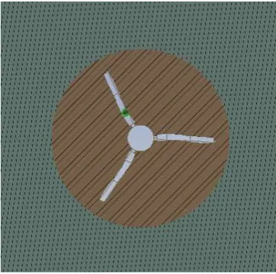
Three separate cylinders were drawn to encompass each blade which was then subsequently separated from the hub part way along the blade pin. A parameter was then added which allowed each blade to be rotated about the centre of the blade pin so that the desired offset for each blade could be set prior to each run without the need for editing the geometry.
To simulate rotor rotation, a Moving Reference Frame (MRF) was used where a rotating component is added to the fluid about the rotational axis of the turbine. To set the MRF, a cylinder of
diameter 0.6 m was created around the turbine, as shown in Figure 1 and Figure 2.). Information was passed between the cylinder and surrounding domain using a domain interface. An angular velocity was assigned to the MRF, corresponding to the required TSR, so that the rotation of the turbine was simulated at each time step.
The total number of elements in the domains was circa 2 million unstructured tetrahedral elements. The rotating domain contained the majority, consisting of 1.5 million elements. Manual mesh refinement, in terms of face sizings, were placed on the blade tip, mid-section, root and hub. The sizing was selected based on the work done by [16] and [20] who extensively modelled the turbine geometry and showed mesh independence. Similarly, the interface between the two domains was refined to produce comparable mesh sizing allowing the preservation of all terms across the interface. These mesh parameters were unchanged for all cases of blade offset.
Fig.2 Turbine geometry for the CFD model
Both a transient and steady-state model were run under the same conditions to determine any difference in performance. The MRF mentioned earlier was used to simulate the rotation of the turbine in both cases. The difference between the two approaches is that the steady-state model is time independent and the mesh is fixed so the turbine is not rotating therefore producing a final single time averaged value. The transient model in comparison allows the performance of the turbine to be monitored with respect to time throughout the rotation, i.e. the turbine and the mesh rotate with respect to the time step.
Table II shows the results from both the steady-state and transient models for a TSR of 3.6, a flow velocity of 1.0 m/s and a pitch of 6°; thus, being the optimum condition (see Table I). The results from the steady-state and transient models are in
close agreement for both CP and CT.
[image:3.595.54.292.421.579.2]were far more computationally expensive the steady-state approach was adopted for the remainder of the models in this study.
TABLEII
COEFFICIENTS OF POWER AND THRUST CALCULATED FROM THE CFDMODEL FOR THE OPTIMUM BLADE PITCH CASE
Model CP CT
Transient 0.439 0.82 Steady-State 0.437 0.817 % of difference 0.45 0.36
B. Blade element momentum theory
As mentioned in Section I, BEMT is the combination of momentum theory and blade element theory which results in a set of equations to compute power and thrust of a TST. These equations cannot be solved unless the lift (Cl) and drag (Cd) coefficients of the aerofoil profile are known. There are different approaches to obtain this data. Depending on the blade profile, some experimental data may be available (e.g. [22]). However, this data often relates to very specific flow velocities and blade geometry. Therefore, another method is to obtain the coefficients numerically with CFD or other existing tools (e.g. Xfoil, Profil 07).
Xfoil is a two-dimensional vortex panel code used to evaluate the flow around aerofoils [23]. Xfoil has been widely used to study aerofoil aerodynamics of aircrafts and renewable energy technology (e.g. wind and tidal turbine blades). Morgado et al. [24] compared Cl and Cd coefficients computed from CFD and Xfoil for two aerofoil types. It was found that Xfoil is accurate in predicting Cl and Cd for high lift aerofoils
at low Reynolds numbers of around 2 . 0 × 1 05. However,
Molland et al. [25] showed that XFoil is capable of predicting Cls within a reasonable margin, but it under predicts Cds,
especially at angles of attack higher than 5°-7°. Similarly,
Porter et al. [11] showed that using Xfoil coefficients at low
Reynolds numbers (Re = 4.4 x 10⁵) resulted in poorer
predictions compared to using experimental data in the model
(Re = 5.1 x10⁴). Even though the authors recognise that Xfoil
is limited in certain aspects, it was used in this study to compute the two-dimensional Cl and Cd coefficients as this information is not available from existing experimental data for the cases considered in this study. Table III gives the Reynolds numbers for the three velocity conditions used in Xfoil.
TABLEIII
REYNOLDS NUMBERS USED IN XFOIL FOR EACH OF THE FLOW VELOCITY CASES
0.9m/s 1.0 m/s 1.1 m/s
9.80E+04 1.10E+05 1.20E+05
The BEMT model used in this investigation was developed at Strathclyde University [26]. To account for some of the limitations of BEMT, Prandtl tip and hub loss correction factors were utilised where the axial/rotational induction factors were modified in the BEMT calculations. To estimate high flow
angles during post stall values, the Viterna-Corrigan method was applied [27].
The work developed in BEMT for this study was based on a simplistic approach to account for blade offsets in a tidal turbine rotor. Therefore, to obtain the power and thrust generated by a turbine with a misaligned blade, separate model runs with different pitch settings were combined linearly. Firstly, the BEMT model was run for the optimal case with a blade pitch of 6°. Then a second run was undertaken with all three of the blades set to the desired offset condition e.g. all blades with 9° or 12° pitch setting depending on the case being modelled (see Table I). Then, according to the studied case, the values of torque and thrust for the optimal and offset cases were combined. For example, a third of the torque (Q) or thrust (T) of the offset case was used in combination with two thirds of the torque or thrust generated by the turbine at optimum conditions. Therefore the overall performance of the turbine, in the case of one blade offset was quantified as:
Qtotal= 1/3Qoffset + 2/3Qopt
Ttotal= 1/3Toffset + 2/3Topt
for a range of TSR values. Similarly for the case with two
blades with different offsets (Case 3, Table I), 1/3rd of each of
the two offset cases and 1/3rd of the optimum case were
combined.
It is the aim of this paper to determine whether such a simplistic, but computationally inexpensive approach can provide a reasonable estimation of turbine performance under these conditions, or whether a more complex, physically based approach is required when modelling misaligned blades. C. Test campaign
In order to assess the results obtained from the BEMT and CFD models, these were compared with the experimental data available in [4]. The tests were carried out at the flume facility at the University of Liverpool with a working section of 1.4 x 0.8 x 3.7 m, using the same 0.5 m diameter turbine, described in Section II-A, as was used in the CFD and BEMT simulations. A blockage ratio of 17% was calculated. The turbine hub centre was installed 0.42 m below still water level. A prior testing campaign carried out by [28] in the facility demonstrated that the flume has a turbulence intensity of about 2% for flow velocities between 0.5 and 1.5 m/s.
A motor was employed to control the turbine by fixing either the rotor speed to the desired value during each test run. Torque was derived by logging the torque generating current generated by the rotor. Additionally, the turbine was equipped with a custom built strain gauging system to measure the forces at the root of one of the blades. Since this system did not incorporate the full rotor, the measurements of root forces were not used in this study. Further information about the test campaign can be found in [5].
III. RESULTS AND DISCUSSION
The first part of this section presents the comparative results between BEMT, CFD and the experimental outcomes. The
coefficients over a range of turbine rotational speeds. Both coefficients were calculated according to the non-dimensional form as described in Section II. The second part of the section
shows the difference in CP and CT between the optimum and
the offset cases.
C. Comparative analysis of power coefficient
Figures 3-5 show the results for CP obtained using BEMT
and CFD of the small scale TST working at 0.9-1.1 m/s. The results were compared to the experimental data obtained in [4].
The BEMT model provides a reasonable prediction of the optimum case compared to the experimental data for each flow condition. The prediction is slightly better for flow velocities of 1.0 and 1.1 m/s which may be related to higher Reynolds numbers and the ability of Xfoil to predict better Cl and Cd data in such flow conditions. The comparison is also reasonable for
the offset Case 1 (offset 9°) and even Case 2 (offset 12°) for
both 1.0 and 1.1 m/s. However, Case 3 (case with two offset blades) presents higher discrepancies when compared to the experimental data. This was to be expected as the three different simulations using blade pitch of 6, 9 and 12 degrees were used to compute Case 3. Thus, the numerical error estimation of each of the cases combine and increase the error in the results. Also, the use of a simplistic approach using BEMT to model the performance of a tidal turbine during off-design conditions is limited when there are large perturbations on the blades. This limitations is perhaps due to wake effects associated with the blade offset that could not be accounted using a linear approach.
For each of the cases, CFD predicts higher CP values than
the experimental data, especially at 0.9 and 1.0 m/s. This discrepancy was seen for the optimum and the offset cases equally. However, the match is slightly better than that obtained from BEMT at 1.1 m/s at peak TSRs.
To visualise the scatter from the experiments, the standard
deviation of CP was included in Figure 6. It can be observed
that for most of the cases, the BEMT prediction is within the standard deviation margins obtained in the experiments. In
comparison, the CP obtained with the CFD model is always
[image:5.595.310.535.64.238.2]higher than the experiments and BEMT. Having higher discrepancies between CFD and the experiments is unexpected. Therefore additional parameters related to the CFD methodology will be explored and discussed in Section III-F.
[image:5.595.321.545.273.446.2]Fig.3 CFD, BEMT and experimental results showing the CP at 0.9 m/s.
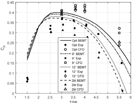
[image:5.595.322.544.480.655.2]Fig.4 CFD, BEMT and experimental results showing the CP at 1.0 m/s.
Fig.5 CFD, BEMT and experimental results showing the CP at 1.1 m/s. CP
CP
Fig.6 Comparative results of CP including the standard deviation values of
the experiments at 1.0 m/s.
D. Comparative analysis of thrust coefficient
The comparative results of CFD and BEMT of thrust coefficients are depicted in Figures 7-9. Compared to the power coefficient, there seems to be a larger discrepancy of the results between the numerical models even for the optimal cases. This
discrepancy increases with the TSR where the CT values
calculated using CFD are about 25% higher at TSR=5.5. As
mentioned before, the experimental CT values from the test
campaign [5] did not seem to be comparable to the simulations done in this study and thus these results are omitted in this section.
It is important to point out that according to the authors’ knowledge; this is the first time that BEMT and CFD have been used to predict the performance of a TST with misalignment in blades. Both numerical methods can be used to predict if a slight blade misalignment has caused detrimental effects in power, which has been argued by [29].
[image:6.595.48.272.74.250.2]Fig.7 BEMT and CFD results showing the CT at 0.9 m/s.
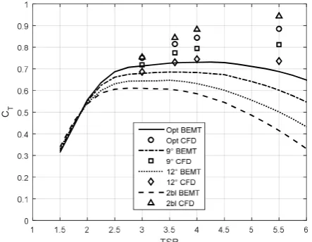
Fig.8 CFD and BEMT results showing the CT at 1.0 m/s.
Fig.9 CFD and BEMT results showing the CT at 1.1 m/s.
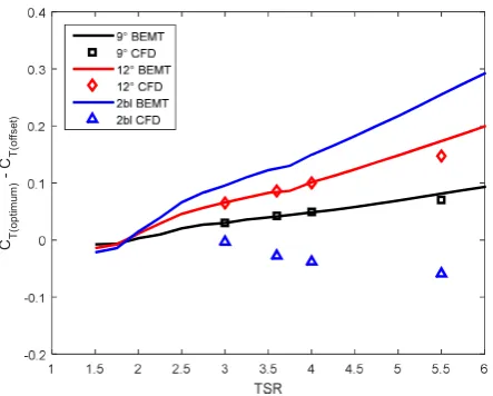
E. Variation of power and thrust coefficients between optimum and offset cases
The difference between the optimum and the offset results is presented in Figures 11-16. This estimation is included to
understand if both models predict the same proportion of CP
and CT lost or gained when the turbine has a misaligned
blade(s).
It can be observed in Figures 11-13 that the same amount of
CP variation is obtained for both numerical models and the
experiments at least for peak TSRs (3<TSR<4) and for the cases with only one misaligned blade and minimal pitch offset (Case 1). Apart from such cases, the experimental data shows higher differences for Cases 2 and 3, compared to the numerical models. Both numerical models show similar variations for Cases 2 and 3 at peak TSRs.
For the CT variation, both numerical models predict similar
differences for the flow velocities of 1.0 and 1.1 m/s and Cases 1 and 2. Higher discrepancies were obtained for the study at 0.9 m/s and Case 3 for each of the flow velocities, again possibly
CP
CT
CT
[image:6.595.312.534.276.450.2] [image:6.595.61.283.511.683.2]due to lower Reynolds Numbers and the complexity of having two misaligned blades with a different offset.
The hypothesis of modelling blade misalignment problems in a BEMT model using a linear solution as a first approximation seems to be an appropriate approach for cases when only one blade presents a small misalignment. The unsteady blade loading and torque that is being developed in the other cases suggests that the problem is non-linear when large perturbations in blade offset are present.
[image:7.595.309.534.62.238.2]The latter should not be a problem when using CFD as this numerical modelling technique treats the problem using a physics based approach. However, given the discrepancies between CFD and the experiments, it was deemed necessary to further analyse the limitations of the CFD model implemented in this study. Therefore, the next section will include additional CFD cases where the effects of control volume, geometry of the turbine, flow speed and changes in boundary conditions are considered.
[image:7.595.47.274.281.457.2]Fig.11 Difference in CP between the optimum and the offset cases at 0.9 m/s.
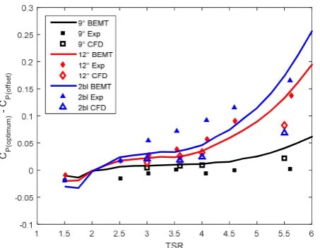
Fig.12 Difference in CP between the optimum and the offset cases at 1.0 m/s.
Fig.13 Difference in CP between the optimum and the offset cases at 1.1 m/s.
Fig.14 Difference in CT between the optimum and the offset cases at 0.9 m/s.
Fig.15 Difference in CT between the optimum and the offset cases at 1.0 m/s. CP
(o
p
tim
um
)
CP
(o
ff
se
t)
CP
(o
p
tim
um
)
CP
(o
ff
se
t)
CP
(o
p
tim
um
)
CP
(o
ff
se
t)
CT
(o
p
tim
um
)
CT
(o
ff
se
t)
CT
(o
p
tim
um
)
CT
(o
ff
se
[image:7.595.311.535.471.644.2] [image:7.595.59.283.490.667.2]Fig.16 Difference in CT between the optimum and the offset cases at 1.1 m/s.
F. CFD simulation analysis
As discussed in the introduction, the level of detail that can be achieved in CFD simulations will depend on the requirements of the model outcomes. Depending on the parameters selected for the model, these will have low/high impact in the solution. In order to better understand the discrepancies between both numerical models, BEMT and CFD, four additional cases were explored using CFD for the optimum pitch setting of 6 degrees and the flow velocity of 1.0 m/s.
The CFD parameters changed in the model described in Section II-A were related to the (i) turbine geometry, (ii) the control volume and (iii) the flow velocity. The turbine geometry was modified by including a stanchion similar to the one used in the experiments. The control volume dimensions were decreased to match the experimental conditions. For the third setting, the flow velocity was increased from 1.0 to 1.5 m/s to investigate the influence of Reynolds number. Finally, the fourth setting investigated in this section was the influence of using the no-slip condition in the simulation that have been used by [14] and [15].
Figures 17 and 18 show the comparison between the original CFD simulations compared to the new cases. The BEMT and experimental values were also included, where possible, to visualise the effects of changing the parameters in the CFD model.
It can be observed that adding the stanchion to the turbine geometry resulted in a decrease of power and thrust coefficient of about 2.6% and 1.5%, respectively. Including the stanchion in the geometry would modify the wake effects and thus affect the performance of the turbine, at this stage the free slip condition was still used. The parameter that influenced the simulation least was the flow velocity. The results between the original simulation at 1.0 m/s and the one at 1.5 m/s only resulted in a difference of 1.5% and 0.5%, respectively. Having a no slip boundary condition using a turbine with and without stanchion also resulted in similar outcomes. However,
changing the control volume, adding a stanchion and using a no slip condition showed a significant improvement on the match between CFD and BEMT. Using this last setting may have a large influence when studying the effects of blade misalignment in a tidal stream turbine and will be considered in future work. Moreover, the implications of using these parameters in a transient simulation may be crucial but these are outside the scope of this study and will be also considered in the future.
[image:8.595.324.545.250.420.2]When these results are again compared to the BEMT simulations, the outcomes of the CFD are still substantially higher than those obtained with BEMT, especially at TSRs>4. It may also be possible that there are wake effects associated with the blade offset that cannot be accounted for with a basic BEMT model. Future research will contemplate the use of a transient BEMT model to account for these effects.
[image:8.595.323.544.447.620.2]Fig.17 BEMT and CFD results showing the CP at 1.0 m/s.
Fig.18 BEMT and CFD results showing the CT at 1.0 m/s.
IV. CONCLUSIONS AND FUTURE WORK
A comparative analysis of CFD and BEMT was carried out to predict the performance of a tidal turbine when it has a misalignment in one or two blades. According to the authors’ knowledge; this is the first time that BEMT and CFD have been
CT
(o
p
tim
um
)
C
T
(o
ff
se
t)
CP
used to predict the performance of a TST with misalignment in blades.
It was found that both CFD and BEMT were able to predict the performance of the turbine for small misalignments of a single blade (3° of incremental pitch) and at flow velocities greater than 1.0 m/s. When looking at the differences between the optimum and offset cases, both numerical models and the
experimental data of CP showed similar variations.
The numerical models showed poorer agreement when
considering the CT values. Both numerical models were also
less effective when computing the CP and CT coefficients with
two offset blades. A simulation analysis to study the effects of changing four parameters in the CFD model showed that including the mounting system in the geometry, setting the control volume to the experimental values and using a no slip condition improves the agreement with BEMT. Thus, future work will focus on exploring the use of these parameters to study blade misalignment performance, including additional cases where transient analysis is carried out.
Similarly, the hypothesis of using a simplistic approach using BEMT to model the performance of a tidal turbine during off-design conditions is not entirely useful when large perturbations exist. Future work will contemplate the use of alternative methods to incorporate blade misalignment in BEMT.
To further validate the numerical models, additional experimental work will be undertaken in the future.
V. ACKNOWLEDGMENTS
The authors would like to acknowledge EPSRC EP/N020782/1 for funding this project.
REFERENCES
[1] Meygen, “The Meygen Project,” Meygen , [Online]. Available: http://www.meygen.com/the-project/. [Accessed 17 March 2017]. [2] A. Kusiak and A. Verma, “A Data-Driven Approach for Monitoring
Blade Pitch Faults in Wind Turbines,” IEEE Transactions on Sustainable Energy, vol. 2, no. 1, 2011.
[3] TidalEnergyToday, “Two turbines up and running at MeyGen,” tidalenergytoday, 12 July 2017. [Online]. Available: http://tidalenergytoday.com/2017/07/10/two-turbines-up-and-running-at-meygen/. [Accessed 12 July 2017].
[4] S. Cacciola, I. M. Agud and C. Bottasso, “Detection of rotor imbalance, including root cause, severity and location,” Journal of Physics: Conference Series 753 (2016) 072003 doi:10.1088/1742-6596/753/7/072003, 2016.
[5] M. Allmark, “Condition Monitoring and Fault Diagnosis of Tidal Stream Turbines Subjected to Rotor Imbalance Faults”, PhD Thesis. Cardiff University, Cardiff Marine Energy Research Group, Cardiff, 2017. [6] I. Masters, J. Chapman, J. Orme and M. Willis, “A robust blade element
momentum theory model for tidal stream turbines including tip and hub loss corrections,” Proceedings of the Institute of Marine Engineering, Science and Technology Part A – Journal of Marine Engineering and Technology, vol. 10, no. 1, pp. 23-35, 2011.
[7] P. Galloway, L. Myers and A. A. Bahaj, “Quantifying wave and yaw effects on a scale tidal stream turbine,” Renewable Energy, vol. 63, pp. 297-307, 2014.
[8] M. Togneri, I. Masters and J. Orme, “Incorporating Turbulent Inflow Conditions in a Blade Element Momentum Model of Tidal Stream Turbines,” in Proceedings of the 21st International Offshore and Polar Engineering Conference, Maui, Hawaii, USA, 2011.
[9] M. G. Gebreslassie, S. O. Sanchez, G. R. Tabor, M. R. Belmont, T. Bruce, G. S. Payne and I. Moon, “Experimental and CFD analysis of the wake characteristics of tidal turbines,” International Journal of Marine Energy, vol. 16, pp. 209-219, 2016.
[10] M. G. Gebreslassie, G. R. Tabor and M. R. Belmont, “Numerical simulation of a new type of cross flow tidal turbine using OpenFOAM– Part II: Investigation of turbine-to-turbine interaction,” Renewable Energy, vol. 50, pp. 1005-1013, 2012.
[11] K. Porter, S. Ordonez-Sanchez, T. Nevalainen, S. Fu and C. Johnstone, “Comparative Study of Numerical Modelling Techniques to Estimate Tidal Turbine Blade Loads,” Singapore, 2016.
[12] C. Frost, C. Morris, A. Mason-Jones, D. O'Doherty and T. O'Doherty, “The effect of tidal flow directionality on tidal turbine performance,” Renewable Energy, vol. 78, pp. 609-620, 2015.
[13] P. B. Johnson, G. I. Gretton and T. McCombes, “Numerical modelling of cross-flow turbines: a direct comparison of four prediction techniques,” in 3rd International Conference on Ocean Energy, Bilbao, Spain, 2010.
[14] M. Lawson, Y. Li and D. Sale, “Development and verification of a computational fluid dynamics model of a horizontal-axis tidal current turbine,” in ASME 30th International Conference on Ocean, Offshore, and Arctic Engineering, Rotterdam, The Netherlands, 2011.
[15] J. Lee, S. Park, D. Kim, S. Rhee and M. Kim, “Computational methods for performance analysis of horizontal axis tidal stream turbines,” Applied Energy, vol. 98, pp. 512-523, 2012.
[16] A. Mason-Jones, “Performance assessment of a Horizontal Axis Tidal Turbine in a high velocity shear,” PhD thesis. Cardiff University, School of Engineering, Centre for Research in Energy Waste and the Environment, Cardiff, 2013.
[17] M. Allmark, P. Prickett, R. Grosvenor, and C. Frost, “Time-Frequency Analysis of TST Drive Shaft Torque for TST Blade Fault Diagnosis.,” presented at the 10th European Wave and Tidal Energy (EWTEC 2015), Nantes, France, 2015.
[18] R. I. Grosvenor, P. W. Prickett, C. Frost, and M. J. Allmark, “Performance and condition monitoring of tidal stream turbines,” presented at the European Prognostic Health Management Conference, Nantes, 2014.
[19] C. Morris, “Influence of Solidity on the Performance, Swirl Characteristics, Wake Recovery and Blade Deflection of a Horizontal Axis Tidal Turbine,” PhD Thesis. Cardiff University, 2014.
[20] C. Frost, Flow Direction Effects On Tidal Stream Turbines. PhD Thesis., Cardiff University, 2017.
[21] R. Howell, N. Qin, J. Edwards and N. Durrani, “Wind tunnel and numerical study of a small vertical axis wind turbine,” Renewable Energy, vol. 35, no. 2, pp. 412-422, 2010.
[22] M. S. Selig and B. D. McGranahan, “Wind Tunnel Aerodynamic Tests of Six Airfoils for Use on Small Wind Turbines,” National Renewable Energy Laboratory, Colorado, USA, 2004.
[23] M. Drela, “XFOIL – an analysis and design system for low Reynolds number airfoils, in: T.J. Mueller (Ed.), Low Reynolds Number Aerodynamics,” Berlin, Springer-Verlag, 1989, pp. 1-12.
[24] J. Morgado, R. Vizinho, M. A. R. Silvestre and J. C. Páscoa, “XFOIL vs CFD performance predictions for high lift low Reynolds number airfoils,” Aerospace Science and Technology, vol. 52, p. 207–214, 2016. [25] A. F. Molland, A. S. Bahaj, J. R. Chaplin and W. M. J. Batten,
“Measurements and predictions of forces, pressures and cavitation on 2-D sections suitable for marine current turbines,” Proceedings of the Institution of Mechanical Engineers Part M Journal of Engineering for the Maritime Environment , vol. 218, no. 2, pp. 127-138, 2004. [26] T. Nevalainen, C. Johnstone and A. Grant, “A sensitivity analysis on
tidal stream turbine loads caused by operational, geometric design and inflow parameters,” International Journal of Marine Energy, vol. 16, pp. 51-64, 2016.
[27] D. A. Spera, Wind Turbine Technology: Fundamental Concepts in Wind Turbine Engineering, Second Edition, New York, USA: ASME, 2009. [28] S. Tedds, I. Owen and R. Poole, “Near-wake characteristics of a model
horizontal axis tidal stream turbine,” Renewable Energy, vol. 63, pp. 222-235, 2014.