Centrality analysis for modified lattices

CENTRALITY ANALYSIS FOR MODIFIED LATTICES

MARTIN PATON∗_{, KEREM AKARTUNALI}†_{,AND DESMOND J. HIGHAM}‡

Abstract. We derive new, exact expressions for network centrality vectors associated with clas-sical Watts-Strogatz style “ring plus shortcut” networks. We also derive easy-to-interpret approxi-mations that are highly accurate in the large network limit. The analysis helps us to understand the role of the Katz parameter and the PageRank parameter, to compare linear system and eigenvalue based centrality measures, and to predict the behavior of centrality measures on more complicated networks.

Keywords: circulant, Katz, network, PageRank, ring, shortcut, spectrum.

AMS Subject Classification: 05C82, 05C50

1. Background and Notation. Algorithms that quantify the importance of nodes in a network are proving to be extremely useful [12, 25, 29]. They allow us to understand hierarchies, discover critical components, and identify targets for deeper investigation. Many of the key ideas behind network centrality measures arose out of the social sciences, where researchers were interested in understanding structural attributes of human interaction networks [13]. The ability to determine who or what is important is also valuable in many application areas, including healthcare, security, advertising, publishing and politics [2,15,21,23].

A key issue, and perhaps a reason for the continued development of new ideas in the field, is that there is no universally-agreed definition (or set of definitions) for importance, and hence no gold-standards for judging centrality measures. So, issues such as validating implementations, understanding the role of algorithm parameters, and comparing centrality measures can only be partially addressed, typically by using real world data sets where some proxy for importance is available, leading to con-clusions that are (a) empirically based and (b) problem-set dependent. In this work, we contribute to the field by showing that there is a synthetic but widely studied “small world” type network for which we can analytically characterize and compare four well-known centrality measures—degree, Katz, eigenvector and PageRank. In particular, we can quantify how the node centralities change as the Katz parameter moves from zero (degree centrality) to its upper limit (eigenvector centrality). More-over, we show how the same techniques allow us to characterize fully these measures on more complex networks where the performance can depend strongly on the choice of Katz or PageRank parameter.

We consider simple unweighted, directed graphs withNnodes. We letA∈_RN×N

denote the adjacency matrix, so thataij = 1 if there is an edge from node ito node

j and aij = 0 otherwise. We also let ρ(A) denote the spectral radius of A, and let 1∈_RN _{denote the vector of ones.}

Section2gives a brief review of Katz, eigenvector and PageRank centrality mea-sures. Section 3summarizes relevant work on Watts-Strogatz style small world net-works and Section4sets up the matrix formulation for our asymptotic analysis. Katz

∗_{Department of Mathematics and Statistics, University of Strathclyde, Glasgow G1 1XH, UK}

([email protected]). Supported by University of Strathclyde Strategic Technology

Partner-ship with CAPITA.

†_{Department of Management Science, University of Strathclyde, Glasgow G4 0GE, UK}

([email protected]). Corresponding author.

‡_{Department of Mathematics and Statistics, University of Strathclyde, Glasgow G1 1XH,}

UK ([email protected]). Supported by EPSRC/RCUK Established Career Fellowship

centrality and eigenvector centrality are analysed in Sections 5 and 6, respectively. In Section 7we apply the same style of analysis to a more general network and find an analytical expression for the parameter cutoff where the ranking from out-degree gives way to that from eigenvector centrality. We also experiment on an extended lattice structure with multiple shortcuts.

Section8gives analysis for PageRank centrality—here the exact solution is found to have a more complicated, non-monotonic, form. We finish in Section9with a brief discussion.

2. Network Centrality Measures. In this section we assume that the network is strongly connected, so that A is irreducible. This property holds for the network class that we study in subsequent sections.

Given A, a centrality measure assigns a value xi > 0 to each node i, with a

larger value indicating a greater level of importance. Typically, it is the ranking of the centrality values that matters—we only care whether one node is more or less important than another, so the vector x ∈ RN is equivalent to βx+γ1 for any

β, γ >0. We summarize here the concepts of Katz, eigenvector and degree centrality, refering to [1, 6, 12, 25, 29] for historical details and discussions of implementation issues. We also consider the PageRank algorithm [14,20,28] which has a different feel; summarizing incoming, rather than outgoing, information, but also assigns a positive real value to each node. Our overall aim is to study, in a specific setting, how changes to the network affect centrality. We note that related questions have been addressed in other contexts; see, for example, [5,11].

Katz centrality [19] defines xvia the linear system

(1) (I−αA)x=1,

whereα∈(0,1/ρ(A)) is a free parameter. Several authors have suggested particular choices forα; see [1] and the references therein. This measure can be motivated by expanding the resolvent (I−αA)−1 _{to give}

x= I+αA+α2A2+α3A3+· · ·

1. Noting that (Ak₎

ij counts the number of distinct walks of length k from i to j, we

see thatxi is a weighted sum of the number of walks from nodeito all other nodes,

where the count for walks of lengthkis scaled byαk_{. Sox}

i is a measure of how well

node ican send information around the network, with more weight given to shorter traversals.

In the limit as α → 0 from above the ranking given by (1) coincides with the ranking from degree centrality, which arises from taking xi to be the out-degree of

nodei; that is,

(2) xi= outdegi, where outdeg =A1.

This makes sense intuitively, since accounting only for the shortest possible walks—of length one—is equivalent to computing the out-degree.

Eigenvector centrality can be motivated recursively, with a node being important if it has links to important nodes. This leads to the expression

(3) xi∝

N

X

j=1

aijxj.

Letting 1/λdenote the constant of proportionality, we may write

(4) Ax=λx,

showing thatxmust be an eigenvector ofAcorresponding to eigenvalueλ. Requiring xi>0 for alliforcesλandxto be the Perron-Frobenius eigenvalue and eigenvector,

respectively.

In the limit as αtends to 1/ρ(A) from below, the Katz centrality vector in (1) gives the same results as the eigenvector centrality vector; see, for example, [4].

The PageRank algorithm, originally proposed in [28], can be motivated from several different perspectives. For example, keeping in mind the context of web pages, we could alter (3) by arguing that the importance of a node is dependent on the importance of the nodes that point to it. Ifaij = 1 indicates a hyperlinkfrom node

i to node j, then we can set up an iteration where each node is given a convex combination of a basal score and a normalized sum of the scores of its followers, so that

x[k+1]_i = 1−d+d

N

X

j=1

aji

outdegj

x[k]_j .

Here, scaling by outdegj ensures that every node has the same opportunity to

dis-tribute its influence across its neighbours. The parameter 0 < d < 1 controls the relative weight given to this redistribution. Taking the limit k→ ∞, we define the PageRank vector as the solution of

(5) I−dATD−1

x= (1−d)1,

whereD= diag(outdegj). We refer to [14,20] for further details.

3. Small World Networks. The seminal work of Watts and Strogatz [30] intro-duced a class of random graphs characterised by having many “local” links and a few “long range” links. Those authors showed, via computational experiments, that such a model can reproduce clustering and pathlength properties that have been observed in real-world complex networks. A key idea in [30] was to add randomness to a regular lattice. Starting from an undirected periodic ring with fixed-range nearest-neighbor connections, the authors introduced a rewiring procedure—each node in the lattice was examined in turn, and, for each of its undirected links, with small independent probability the end point of that link was replaced by another node chosen uniformly at random. In terms of developing analytical results to back up the observations in [30], the rewiring process presents difficulties; for example, a node may become isolated with nonzero probability. For this reason, subsequent research focused on a slight variation where existing edges are not altered, but new edges, termedshortcuts, are added between randomly selected nodes in the network. For example, focusing on theN → ∞limit, [24,26,27] develop heuristic approximations and [3] gives rigorous results. Markov chain versions with hitting time as a proxy for pathlength were also studied rigorously in [10, 16,17,31]. Of particular relevance to our study is the ref-erence [22], which analysed the effect of shortcuts on the underlying matrix spectrum from a linear algebra viewpoint.

eigenvalue centralities is not interesting. This can be seen from the following simple lemma.

Lemma 1. Suppose that all nodes in a network have the same out-degree. Then all nodes have the same Katz centrality measure. Similarly, assuming strong connectivity, all nodes have the same eigenvector centrality measure.

Proof. We have

(6) A1= od1,

where od≡outdegidenotes the common out-degree. Hence1is the Perron-Frobenius

eigenvector and ρ(A) = od. Any Katz parameter 0 < α <1/od is valid, and we see from (6) thatx=1/(1−αod) solves the Katz system (1).

4. Matrix Modification. Let C ∈ RN×N be the adjacency matrix for the

periodic nearest neighbour ring; so in theN = 6 case,

(7) C=



      

1 1

1 1

1 1

1 1

1 1

1 1



       .

We note that C is symmetric and circulant, and standard theory shows that the Perron-Frobenius eigenvalue is ρ(C) = 2 with corresponding eigenvectorx =1[18, page 100], which, from Lemma1, also solves the Katz system (1), up to a multiplicative factor, for any 0< α <1/ρ(C). It is, of course, intuitively reasonable that all nodes in this network should be assigned the same centrality value in (1), (2) and (4).

Next we add a single directed shortcut. Without loss of generality we give the shortcut to node 1 and let L be the index of the target node. So our adjacency matrixAin (1) has the formA=C+E, where the rank one matrixE is zero except for E(1, L) = 1. Liu, Strang and Ott [22] describe this as a modification of C, to emphasize that we have an O(1) change in a matrix entry, rather than the type of small change studied in classical matrix perturbation theory. These authors studied the eigenvector associated with the dominant eigenvalue of A, and related matrices, and constructed accurate approximations to this vector. Further work concerning the eigenvalues arising from general modifications to structured matrices has appeared in, for example, [7,8,9].

Our work is strongly motivated by [22] but differs from it in three respects.

• Rather than deriving small residual approximations and then using stability arguments to bound the forward error, we construct exact solutions that can be expanded asymptotically. This more direct route leads to shorter proofs and sharper bounds.

• We consider Katz and PageRank centrality (as well as the eigenvalue prob-lem).

• We interpret the results from a network science perspective and show how they can give new insights about behavior on more complicated networks. For convenience, we letp(i) for any 1≤i≤N denote the periodic distance from nodeito node 1, that is,

1 5 10 15 20

Node Index

2.5 3 3.5

Katz & Approx.

Katz

Dominant Term

1 5 10 15 20

Node Index

10-10 10-5

Discrepancy

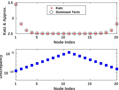
Fig. 1.Upper picture: asterisks show components of Katz vector from (1) and circles show the approximationb+h1tp1(i)from (12). Hereb= 1/(1−2α),t1is defined in (11) andh1 was found by

solving (20). Lower picture: the discrepancyxi−b−h1tp₁(i) on a log scale. From Theorem1, this

quantity has the formh2tp2(i), and hence grows geometrically away from the shortcut node. However,

it is uniformlyO(tN/1 2)for a fixed0< t1<1, and hence rapidly becomes negligible as the network

sizeN increases.

We can assume without loss of generality that the receiving nodeLis not beyond the half way, or “six o’clock”, position on the ring. We are interested in large networks with long-range shortcuts. So, letting b·c denote the integer part, for some fixed proportion 0< θ≤1 we set

(9) L=

(

bθ(N/2 + 1)c whenN is even,

bθ(N+ 1)/2c whenN is odd.

We note thatL→ ∞asN → ∞.

5. Katz Centrality. In the upper picture of Figure1, the asterisks show Katz centrality values for a network with adjacency matrixA=C+E, that is, components ofxfrom (1). We chose a small network size in order to make the key effects visible. More precisely, we used an N = 20 node ring with a shortcut from node 1 to node L = 8, for α= 0.3. Because node 1 owns the extra, long-range edge, it attains the highest centrality score, at around 3.5. The most distant node, periodically, node 11, is deemed the least central. Insight from [22], or from eyeballing the solution, suggests that components ofxi, when suitably shifted, might be varying geometrically as the

indeximoves periodically around the ring; that is xi=b+htp(i)for some constants

b, h > 0 and 0< t <1. Fitting an ansatz of this form leads us to the circles in the upper picture of Figure1. The agreement is close—below 2×10−5_{in Euclidean norm.}

The lower picture in Figure1shows, on a log scale, the discrepancy between those asterisks (true solution) and circles (geometric decay ansatz). We see a very small contribution that, in contrast to the overall solution,grows geometrically as we move periodically away from node 1.

N → ∞with a fixed Katz parameter 0< α <1/2. This upper limit forαis chosen because, as proved in section10,ρ(A) tends to 2 from above asN → ∞.

Theorem 1. For the undirected ring plus directed shortcut network with adja-cency matrix A = C+E, for sufficiently large N the unique solution of the Katz system (1) has the form

(10) xi=b+h1t

p(i) 1 +h2t

p(i) 2 .

Here, b, t1, t2, h1, h2 are constants, i.e., independent of i, and b, t1, t2 are also

inde-pendent of N. In particular, h1>0, h2 >0,b= 1/(1−2α)and t1, t2 are the roots

of the palindromic quadratic αt2−t+α, so that

(11) t1=

1−√1−4α2

2α , t2=

1 +√1−4α2

2α ,

witht2= 1/t1 and0< t1<1< t2. Moreover, the final term in (10) is exponentially

small asymptotically, in the sense that for all 1≤i≤N,

(12) xi=b+h1t

p(i) 1 +O(t

N/2 1 ),

withh1=O(1).

Proof. Because the quadratic is palindromic,t1andt2in (11) must satisfyt1t2=

1. It is clear that these roots are real, with 0< t1<1< t2, and we note the further

useful facts

(13) 1−2αt1=

p

1−4α2_{>0, 1−2αt} 2=−

p

1−4α2_<0

and

(14) t1−2α

t2−2α

=−t21.

Consider the case where the number of nodes, N, is even. We begin with the ansatz

(15) xi=b+htp(i).

The Katz system (1) essentially reduces to three scalar equations. At a general nodek, corresponding to thekth row of the linear system, fork6= 1 andk6=N/2 + 1 we have

(16) −αxk−1+xk−αxk+1= 1.

Inserting (15), this becomes

b(1−2α) +htp(k)[1−αt−α/t] = 1.

We can satisfy this equation independently ofkby settingb= 1/(1−2α) and choosing t to be either root of the quadraticαt2_{−t+α. By linearity of (16), we may extend}

(15) to include a linear combination involving both roots, so our ansatz becomes

(17) xk =b+h1t

p(k) 1 +h2t

p(k) 2 .

The two remaining equations to satisfy from (1) arise at nodes 1 and N/2 + 1, where we require

(18) −αxN+x1−αx2−αxL= 1

and

(19) −αxN/2+xN/2+1−αxN/2+2= 1,

respectively. Inserting (17) into (18) and (19), usingb(1−2α) = 1, we have the linear system

(20)

"

1−2αt1−αtL1−1 1−2αt2−αtL2−1

tN/2₁ −1(t1−2α) t N/2−1

2 (t2−2α)

# h1

h2

=

bα

0

.

To prove that a solution of the form (17) exists, we now show that this system is nonsingular. The determinant may be written

(21) 1−2αt1−αtL1−1

tN/2₂ (1−2αt1)− 1−2αt2−αtL2−1

tN/2₁ (1−2αt2).

Recalling that 0< t1<1< t2, we see from (13) that, asN→ ∞and henceL→ ∞,

the first term in (21) becomes, to leading order,

(1−2αt1) 2

tN/2₂ → ∞.

The second term in (21) becomes, to leading order,

(22) αtL₂−1tN/2₁ (1−2αt2) =αt N/2−L

1 (t1−2α).

Recall thatL=bθ(N/2 + 1)c, so

N/2−L > N/2−θ(N/2 + 1) = (1−θ)N/2−θ.

Hence, asN→ ∞, termαtN/2₁ −L(t1−2α) in (22) is bounded forθ= 1, and tends to

zero forθ <1. So the first term in (21) dominates, and the determinant is bounded away from zero for largeN.

We have shown that for sufficiently largeNthe unique solution of the Katz system (1) has the form (17). We now follow up by showing that, in the exact solution (17), the growing termh2t

p(i)

2 is negligible for largeN.

From the second equation in (20), we have, using (14),

(23) h2=h1tN1.

Hence, in the first equation of (20),

h11−2αt1−αtL1−1−αt N−L+1 1 −2αt

N−1 1 +t

N 1

=bα.

We see thath1=O(1). Also, using (13), we deduce thath1>0 for largeN. It then

follows from (23) thath2>0 andh2=O(tN1 ). Since the termh2t p(k)

2 is largest when

k=N/2 + 1, we also see that

xi=b+h1t p(i) 1 +O(t

N/2 1 ).

1 10 20 30 40

Node Index

0 0.2 0.4

Eig & Approx.

Eigenvector Dominant Term

1 10 20 30 40

Node Index

-0.02 0 0.02 0.04

Discrepancy

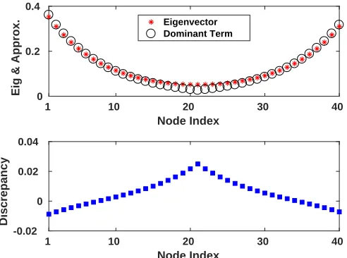
Fig. 2. Upper picture: asterisks show components of the Perron-Frobenius vector and circles show the approximation sp₁(i) from (24), with s1 defined in (25). Both vectors are normalized to

have unit Euclidean norm. Lower picture: the discrepancy. From Theorem2, xi−sp1(i) has the

formsN₁−p(i), and hence grows geometrically away from the shortcut node.

6. Eigenvector Centrality. This section looks at eigenvector centrality for the matrix C +E. We note that ρ(C+E) ≤ ||C+E||∞ = 3. Also, it is true in general that adding an edge to a strongly connected network strictly increases the spectral radius; see [18, Problem 8.4P14]. So 2 < ρ(C +E). From the network centrality perspective, we are concerned mainly with the structure of the Perron-Frobenius eigenvector. However, for completeness, in Section10 we establish a tight bound on the corresponding eigenvalue.

The asterisks in the upper picture of Figure2show the components of the Perron-Frobenius vector for A =C+E in the case whereN = 40 andL = 12. As in the Katz case seen in Figure1, there is evidence of periodic geometric decay. The circles in the picture show an ansatz of the formxi=s

p(i)

1 for 0< s1<1. Both vectors were

normalized to have unit Euclidean norm. The lower picture shows the discrepancy between the two, and again we see a small contribution that increases periodically away from node 1.

Theorem2makes these observations concrete. The result is strongly motivated by the approach in [22], where exponentially accurate approximations were constructed. We extend this approach in order to obtain an explicit expression for the Perron-Frobenius eigenvector. The technique of proof is similar to that in Theorem1. How-ever, we point out that whereas the Katz parameter α in Theorem 1 is fixed, the Perron-Frobenius eigenvalueλin Theorem2 is dependent uponN.

Theorem 2. For the undirected ring plus directed shortcut network with adja-cency matrix A =C+E, let λ denote the Perron-Frobenius eigenvalue. Then, for sufficiently largeN, we have2< λ <5/2and the Perron-Frobenius eigenvectorxhas the form

(24) xi=s

p(i) 1 +s

p(i)−N

2 ,

wheres1, s2 are the roots of the palindromic quadratics2−λs+ 1, so that

(25) s1=

λ−√λ2₋₄

2 , s2=

λ+√λ2₋₄

2 ,

withs2= 1/s1 and0< s1<1< s2.

Proof. SupposeN is even.

Following the proof of Theorem1, we start with the ansatzxi =b+hsp(i)for the

eigenvector, and attempt to satisfy the requisite equations for the general node, for node 1 and for nodeN/2 + 1.

At a general nodek, that is, in thekth row of (4), we require

b(2−λ) +hsp(k)(1/s+s−λ) = 0.

This may be satisfied by setting b to zero and sto the value s1 or s2. By linearity,

we therefore continue with

(26) xi=h1s

p(i) 1 +h2s

p(i) 2 .

Since the eigenvector is only unique up to a scaling, we seth1= 1, leavingh2 andλ

as free parameters. The conditions in (4) corresponding to nodes 1 andN/2 + 1 may be written

(2s1−λ+sL1−1) +h2(2s2−λ+sL2−1) = 0,

(27)

sN/2₁ (2s2−λ) +h2s N/2

2 (2s1−λ) = 0,

(28)

respectively. Sinces1= 1/s2, multiplying (28) by a factor ofs N/2

2 we obtain

h2=s−2N

−(2s2−λ)

2s1−λ

=s−₂N −

√

λ2₋₄ −√λ2₋₄

!

=s−₂N.

Then writing (27) in terms of the remaining unknown, λ, we have

(29) F(λ) = 0,

where

F(λ) =−pλ2₋₄



1− λ−

√

λ2₋₄

2

!N

+

λ−√λ2₋₄

2

!L−1

+ λ−

√

λ2₋₄

2

!N−L+1 . (30)

It is straightforward to show thatF(2)>0, whereas atλ= 5/2 we have

F(5/2) =−3

2 1−2 −N

+ 21−L+ 2L−N+1

=−3

2+O(2 −θN/2

) +O(2−(1−θ)N/2)<0,

for largeN. So the continuous functionF changes sign in the interval (2,5/2). We have thus established that the nonsymmetric matrix C+Ehas an eigenvec-tor of the form (24) with an eigenvalue in (2,5/2). We can rule out the possibility of an eigenvector existing that has a larger eigenvalue. This follows from [18, Prob-lem 8.4.P15] (which applies to all nonnegative, irreducible matrices)—because we have constructed an eigenvector with allxi>0, it must be a Perron-Frobenius eigenvector.

7. Extensions.

7.1. Multiple Rings. The results from Theorems 1 and 2 give exact charac-terizations of the centrality vectors, and the presence of both geometrically decaying and geometrically increasing components is not intuitively obvious. However, the qualitative nature of the solution, with most weight given to the node with the high-est out-degree and with overall centrality decaying according to periodic distance from this node, is no surprise. In this subsection, we show that the type of analysis developed here can be applied to a more general network where the results are not predictable. To our knowledge, this is the first example to capture analytically (rather than experimentally) a change in node centrality ranking as the Katz parameter is varied. To isolate the key ideas, we have chosen a simple network structure, but we note that the same approach can be applied in more general settings.

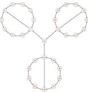
We study a network built from three undirected, periodic, nearest neighborm -node rings. Nodes 1 tom, nodesm+ 1 to 2mand nodes 2m+ 1 to 3mmake up rings one, two and three, respectively. Node 1 is given a long range directed shortcut to nodeL, where 1L≤m/2 + 1. Similarly, nodesm+ 1 and 2m+ 1 are given long range directed shortcuts to nodes m+ 1 +Land 2m+ 1 +L, respectively. An extra node, with index N = 3m+ 1, is then introduced and connected by an undirected edge to the nodes that have shortcuts. Figure 3 illustrates the case where m = 10 andL= 5.

By symmetry, we only need to consider Katz centrality for nodes in the first ring, that is, nodes 1 to m, and for the additional node,N. We note that node 1 has out-degree four, whereas nodeN has out-degree three. It follows that for smallα, node 1 will have the higher Katz centrality. However, the three edges possessed by node N connect to nodes that are themselves well-connected, and can propagate more walks round the network than other nodes on the ring. This suggests that asαis increased, and hence longer walk counts become more relevant, Katz centrality may give more relative weight to nodeN. Our aim is to quantify this effect.

We use the ansatz in Theorem 1, but rather than deriving an exact solution, we focus on the dominant terms. For this network, the Katz system (1) reduces to

xj−α(xj−1+xj+1) = 1, for 2≤j≤m,

(31)

x1−α(xm+x2+xL+xN) = 1,

(32)

xN−3αx1= 1.

(33)

Inserting the ansatz (15) we find that, as in the proof of Theorem 1, the general equation (31) is solved withb= 1/(1−2α) andt=t1. UsingxL≈band solving (32)

and (33) forh, we arrive at

(34) h≈ α(2 +α)

(1−2α)(1−2αt1−3α2)

.

As αincreases away from zero, the expression (34) is initially positive and changes sign on crossing a pole where

α=αb:= p√

13−2

3 ≈0.4224.

In passing, we therefore conjecture that the adjacency matrix for this network has a spectral radius that approaches 1/α_b as N → ∞and hence the Katz system is valid

1 2 3 4 5

6

7

8

9 10

11

12 13

14 15 16 17 18

19

20

21 22

23

24

25 26

27 28 29 30 31

Fig. 3. Illustration of the three-ring undirected network where a directed shortcut is added to each ring, and an extra node is added and given undirected connections to the shortcut nodes. This shows the casem= 10, so thatN= 31, andL= 6.

for 0 < α < α_b. Using x1 = b+h and, from (33), xN = 1 + 3αx1, it follows that

xN > x1 when

(35) (1−2α)(1−2αt1−3α

2_{) + (3α−1)(1 + 2α(1−t} 1−α))

(1−2α)(1−2αt1−3α2)

>0.

For 0 < α < α_b the denominator in (35) is positive and the condition reduces to α > α?_{, where}

(36) α?= 10−

√

13

29 ≈0.2205.

In summary, we claim that, asymptotically, α? _{is the threshold value beyond which}

nodeN is regarded as more central than node 1.

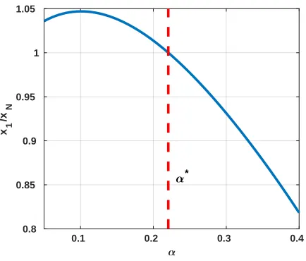
Figure4supports this conclusion by plotting the ratiox1/xN asαis varied. We

used m = 10,000, so N = 30,001, withL = 5,001 and solved the Katz system (1) directly. We see that α? _{in (36), marked with a vertical dashed line, predicts the}

crossover point where xN becomes dominant. It is also interesting to observe that

x1/xN is not monotonic inα. As further confirmation of the analysis, we found that

0.1 0.2 0.3 0.4 0.8

0.85 0.9 0.95 1 1.05

x1

/x

N

*

Fig. 4. Ratio of x1 toxN for Katz centrality on theN = 30,001version of the network in Figure3. The predicted thresholdα?_{is marked as a vertical dashed line.}

computed values shown in the figure to machine precision. Also, the spectral radius of the adjacency matrix, computed via MATLAB’seigs, matched 1/α_bto within 10−13_.

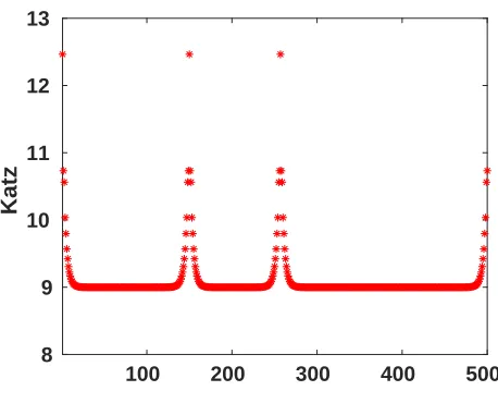
7.2. More Neighbors and Shortcuts. Next, we indicate briefly how the anal-ysis in Section 5 may be generalized to rings with more neighbors and shortcuts. Figure 5 shows Katz centrality, withα= 1/4.5, for a network based on a 500 node periodic ring where each node is connected to two clockwise and two counterclock-wise neighbors. Three arbitrary, long-range, directed shortcuts were added: 17→200, 150 7→ 390 and 257 7→ 450. We can see from Figure 5 that nodes 1, 150 and 257 benefit from their extra edge, and the centrality vector has a spike at each of the three locations.

To describe this behavior, consider a general node kthat is close to node 1, but for whichk6= 1,2, N. Then the Katz system (1) for this node has the form

xk−α(xk+1+xk+2+xk−1+xk−2) = 1.

Using the ansatz xi = b+hrp(i), we find that this equation is solved by taking

b= 1/(1−4α) andr2_−α(r4_+r3_{+r+ 1) = 0. That palindromic quartic polynomial}

has four real roots

rA≈0.73, rB≈ −0.37, rC≈1.37, rD≈ −2.73.

As for the three-ring example, we proceed by focusing on the decaying terms, corre-sponding to roots with absolute value less than one, assuming that the growing terms will be negligible. At nodes 1 and 2 (we could equivalently use 1 andN), we require

x1−α(x2+x3+xN +xN−1+x200) = 1 and x2−α(x3+x4+x1+xN) = 1,

respectively. Insertingx200=b and, otherwise,xi=b+hAr p(i) A +hBr

p(i)

B , we obtain

the linear system

1−α(2rA+ 2r2A) 1−α(2rB+ 2rB2)

rA−α(1 +rA+rA2 +r3A) rB−α(1 +rB+r2B+rB3)

hA

hB

=

bα

0

.

100 200 300 400 500 8

9 10 11 12 13

Katz

Fig. 5.Components of Katz centrality vector for a500node periodic ring with two connections on each side and directed shortcuts added to nodes1,150and257.

This solves to givehA≈2.73 andhB ≈0.73.

To cover all the shortcuts, we superimpose three such spikes, so

xi≈b+hAr p(i) A +hBr

p(i) B +hAr

p150(i) A +hBr

p150(i) B +hAr

p257(i) A +hBr

p257(i)

B ,

wherepL(i) denotes the periodic distance from nodeito node L; that is

(37) pL(i) = min (|i−L|,|N−i+L|).

This approximation agreed with the computed Katz centrality vector to within 2×

10−7 _{in each component. After normalizing both vectors to unit Euclidean norm, the}

maximum componentwise discrepancy fell below 10−9_.

8. PageRank. We now consider the PageRank system (5) on a periodic ring plus a directed shortcut. To be consistent with the treatment in sections 5 and 6, we will ensure that node 1 remains the most highly ranked. So the directed shortcut will be addedfrom nodeL to node1. Hence, the adjacency matrix now has the form A=C+Eb, where the rank one matrixEbis zero except for E(L,1) = 1.

Figure 6 relates to the case whereN = 20,L= 8 and d= 0.8. Asterisks in the upper picture show the components of the PageRank vector x in (5). We see that node 1 is ranked highest, and node L, which gives away the extra shortcut, has a low ranking that is slightly higher than its two neighbours. Unlike the cases shown in Figures1 and2, the solution does not appear to be periodically symmetric about node 1.

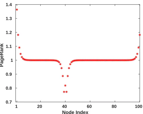
Figure7gives a view of the asymptoticN → ∞structure by increasingNto 100, with L = 40. The solution now appears to be periodically decreasing locally away from node 1 and periodicallyincreasing locally away from nodeL.

1 5 10 15 20

Node Index

0.5 1 1.5

PgR & Approx.

PageRank Dominant Term

1 5 10 15 20

Node Index

-5 0 5

Discrepancy

10-4

Fig. 6. Upper picture: asterisks show components of the PageRank vector x from (5) and circles show the periodic spike approximation (40)–(41). Lower picture: the discrepancy between these two vectors.

shows the discrepancy, which takes relatively small values that peak and trough at the nodes diametrically opposite 1 andL, respectively. We also see in Figures6and 7that nodeLdoes not quite fit into the general pattern of periodic growth/decay.

The solutions seen in Figures6and7may be likened to a positive spike centered at node 1 plus a negative spike centered at nodeL, so we may expectxito contain a

term proportional to up(i)₁ and a term proportional to −upL(i)

1 , where we recall that

pL(i) in (37) denotes the periodic distance from nodeito nodeL.

An exception occurs at node L, which seems to break this pattern. Theorem 3 below shows that the solution does indeed have this general form—plus exponentially small terms—with a simple shift needed at node L. The general form (38)–(39) involves five constantsg1, g01, g2, g20, f and our proof technique relies on five “special”

nodes that impose independent constraints. For this reason, we need to rule out the exceptional case where nodeLis within one hop of being diametrically opposite node 1, which would lead to fewer than five special nodes. We therefore assume that the shortcut is chosen so that 0< θ <1 in (9). We also treat the PageRank parameter 0< d <1 as being fixed, independently ofN.

Theorem 3. For the undirected ring plus directed shortcut network with adja-cency matrix A = C +E, forb 0 < θ < 1 and for sufficiently large N the unique solution of the PageRank system (5) has the form

(38) xi = 1 +g1u p(i) 1 +g2u

p(i) 2 +g

0

1u pL(i)

1 +g

0

2u pL(i)

2 , fori6=L,

and

(39) xL= 1 +g1u1L−1+g2uL2−1+g

0

1+g20 +f.

Here, u1, u2, g1, g2, g10, g02, f are constants, i.e., independent ofi, andu1, u2 are

inde-pendent ofN. In particular,g1>0,g2>0,g01<0,g02<0,f >0, andu1, u2 are the

1 20 40 60 80 100

Node Index

0.7 0.8 0.9 1 1.1 1.2 1.3 1.4

PageRank

Fig. 7. Asterisks show components of the PageRank vector xfrom (5) for a larger network: hereN= 100andL= 40.

roots of the palindromic quadraticdu2_{−2u+d, so that}

u1=

1−√1−d2

d , u2=

1 +√1−d2

d .

Hence, u2 = 1/u1 and 0 < u1 < 1 < u2. Moreover, the terms in (38) and (39)

involvingg2 andg02 are exponentially small asymptotically, in the sense that

xi= 1 +g1u p(i) 1 +g

0

1u pL(i)

1 +O(u θN/2

1 ), fori6=L,

(40)

xL= 1 +g01+f+O(u θN/2 1 ).

(41)

We also have

g1=

d

1 + 2√1−d2 +O(u θN/2 1 ),

(42)

g0₁= −1

1 + 2√1−d2 +O(u θN/2 1 ),

(43)

f =

√

1−d2

1 + 2√1−d2 +O(u θN/2 1 ).

(44)

Proof. As in the proofs of Theorems1and2, we show by direct substitution that xsatisfies the required conditions. Because the style of analysis is similar, we omit some of the fine details.

Assume thatN is even.

For a general nodek, the PageRank system (5) requiresxk−d(xk−1+xk−1)/2 =

• node 1, where there are three incoming edges,

• node L, where, from (39), the general form of the solution has undergone a shift,

• nodeL+ 1 (or, equivalently, nodeL−1), where the nonstandard node Lis involved,

• nodeN/2 + 1, which has neighbours that are the same periodic distance from node 1,

• nodeN/2 +L, which has neighbours that are the same periodic distance from nodeL.

Our equation for node 1 isx1−d(x2/2 +xN/2 +xL/3) = 1−d. Using (38) and

(39), and simplifying, we arrive at

(45) g1 1−d u1+13u L−1 1

+g2 1−d u2+13u L−1 2

−1 3d(g

0

1+g

0

2+f + 1) = 0.

For nodeL, we havexL−d(xL−1/2 +xL+1/2) = 1−d, which simplifies to

(46) g₁0(1−du1) +g02(1−du2) +f = 0.

NodeL+ 1 givesxL+1−d(xL/3 +xL+2/2) = 1−d, from which we obtain

(47) g1uL1−1+g2uL2−1+g

0

1+g

0

2−2f =−1.

At nodeN/2 + 1 we havexN/2+1−d(xN/2/2 +xN/2+2/2) = 1−d, which leads to

(48) g2=g1uN1.

Similarly, at nodeN/2 +L, the condition xN/2+L−d(xN/2+L−1/2 +xN/2+L+1/2) =

1−dleads to

(49) g₂0 =g0₁uN₁.

Using (48) and (49) to eliminateg2andg20, we are left with three linear equations,

(45)–(47), for the three unknownsg1,g10 andf. These may be written in the form

(50) (B+ ∆B)v=r,

where

B = 



1−du1 −d/3 −d/3

0 1−du1 1

0 1 −2



, v= 

 g1

g₁0 f



, r= 

 d/3

0

−1 

,

and ∆B ∈ R3×3 is such that k∆Bk∞ = O(u

θN/2

1 ). Writing u1 in terms of d, the

determinant ofB reduces to−(1 + 2√1−d2₎√_1−d2_{6= 0, soB is nonsingular.}

From (50), we have

I+B−1∆Bv=B−1r.

The matrixI+B−1_{∆Bis invertible for sufficiently largeN, which establishes that (50)}

has a unique solution. We conclude that xin (38)–(39) solves the PageRank system (5). Moreover, since (I+B−1_∆B)−1_{=I+O(∆B), we see thatv=B}−1_r+O(uθN/2

1 ),

which leads to (42)–(44). The relations (48) and (49) then show thatg2>0 andg20 <0

and also give the expansions (40) and (41). The result forN odd follows similarly.

For the examples in Figures6and7, we see that the node giving out the extra link, with indexL, has a slightly larger PageRank value than its immediate neighbors, but not more than its second-neighbors. The following corollary shows that this behavior is generic.

Corollary 1. For the undirected ring plus directed shortcut network with adja-cency matrixA=C+E, for sufficiently largeb N the PageRank vector satisfies

max (xL+1, xL−1)< xL<min (xL+2, xL−2).

Proof. It follows from Theorem3that, ignoring asymptotically small terms,

xL= 1 +g01+f, xL+1=xL−1= 1 +g10u1, xL+2=xL−2= 1 +g10u 2 1.

Using (42), (43) and (44) we find that

xL−xL+1=xL−xL−1=

(1−d) 1−√1−d2 d(1 + 2√1−d2₎ >0,

and

xL−xL+2=xL−xL−2

−√1−d2 √_1−d2₋₁2 d2_{(1 + 2}√_1−d2₎ <0.

We can at least partially explain the ordering in Corollary1by noting that nodes L+ 1 andL−1 suffer because one of their two neighbors, nodeL, has three outgoing links. Hence the “vote of confidence” from nodeLis split three ways instead of two. As a consequence, nodeLitself suffers from having two lowly-ranked neighbors. What is perhaps less obvious, but proved in Corollary1, is that nodesL−1 and L+ 1 can never rise above nodeL, which itself can never rise above nodesL−2 andL+ 2.

9. Discussion. In this work, we have addressed issues in matrix analysis con-cerning modified rings. In particular, we have extended the approximation technique from [22] in order to give exact solutions, and applied these ideas to spectral and linear system problems arising in network science, where the matrix modifications correspond to shortcuts in the classic Watts-Strogatz model. The results give a com-plete understanding of the structure of the centrality vectors on this class, and in the case of PageRank centrality they reveal an unexpected nonmonotonicty in the rank-ings. We also showed how the same techniques can be used to study more general networks where the node ranking is not predictable in advance.

There is clearly much potential for further work in this area. An immediate issue is the rigorous treatment of the generalk-neighbor ring, which would involve an understanding of the roots of the palindromic polynomialrk_−α(r2k_{+· · ·+r}k+1₊

rk−1_{+· · ·+1). Furthermore the questions addressed here could be posed on (a) higher}

dimensional lattices, such as nearest-neighbor connections on a torus, (b) hierarchical “network of network” structures, or (c) non-periodic lattices where boundary effects may be significant. Multiple shortcuts could be included, with various asymptotic scalings for their length and separation. Also, in the spirit of [30], random shortcuts could be analysed in a suitable probabilistic framework.

Theorem 4. Given any > 0 and K > 0, for sufficiently large N the Perron-Frobenius eigenvalueλin Theorem 2is such that

2 + K

N2 < λ <2 +

K N2−.

Proof. We consider the caseN even, and investigate the roots ofF(λ) in (30). If λhas the form

λ= 2 +KN−β

for someβ >0, then to leading order in (25) we have

s1= 1−K1/2N−β/2+O(N−β),

(51)

s2= 1 +K1/2N−β/2+O(N−β).

(52)

Now supposeβ = 2. Recalling thatLis proportional toN, we have

logsL₁−1 = (L−1) log1−K1/2N−1+O(N−2)

= (L−1)−K1/2N−1+O(N−1)

→ −γK1/2,

for some fixedγ. So

sL₁−1→e−γK1/2. Similarly,

sN₁−L+1→e−(1−γ)K1/2 and sN₁ →e−K1/2. SinceF(λ) in (30) may be written

F(λ) = (2s1−λ)(1−sN1) +s L−1 1 +s

N−L+1

1 ,

we conclude that it takes the form of an asymptotically small negative term plus positive terms that are bounded away from zero. HenceF(λ)>0 for largeN.

Now supposeβ <2. Similar analysis shows that, asN → ∞,

s₁L−1→0, s₁N−L+1→0, sN1 →0,

at rates that are exponential; that is, as fast as e−νN1−β/2 _{for some fixed ν > 0. It}

follows that F(λ) in (30) is dominated by the term −2√KN−β/2_{, so F(λ) <0 for}

sufficiently largeN.

The case whereN is odd can be treated in a similar manner.

AcknowledgementsWe thank two reviewers for very detailed feedback on our initial submission.

REFERENCES

[1] M. Aprahamian, D. J. Higham, and N. J. Higham,Matching exponential-based and resolvent-based centrality measures, Journal of Complex Networks, 4 (2016), pp. 157–176, https:

//doi.org/10.1093/comnet/cnv016.

[2] S. Aral,Social science: Poked to vote, Nature, 489 (2012), pp. 212–214,https://doi.org/10.

1038/489212a,http://dx.doi.org/10.1038/489212a.

[3] A. Barbour and G. Reinert,Small worlds, Random Structures and Algorithms, 19 (2001), pp. 54–74.

[4] M. Benzi and C. Klymko,On the limiting behavior of parameter-dependent network centrality measures, SIAM J. Matrix Anal. Appl., 36 (2015), pp. 686–706.

[5] P. Boldi, A. Luongo, and S. Vigna,Rank monotonicity in centrality measures, tech. report, 2017,http://vigna.di.unimi.it/ftp/papers/rank.pdf.

[6] F. Bonchi, P. Esfandiar, D. F. Gleich, C. Greif, and L. V. Lakshmanan,Fast matrix computations for pairwise and columnwise commute times and Katz scores, Internet Math-ematics, 8 (2012), pp. 73–112.

[7] A. B¨ottcher, M. Embree, and M. Lindner,Spectral approximation of banded Laurent ma-trices with localized random perturbations, Integral Equations and Operator Theory, 42 (2002), pp. 142–165.

[8] A. B¨ottcher, M. Embree, and V. I. Sokolov, On large Toeplitz band matrices with an uncertain block, Linear Algebra and its Applications, 366 (2003), pp. 87–97.

[9] A. B¨ottcher, M. Embree, and V. I. Sokolov,The spectra of large Toeplitz band matrices with a randomly perturbed entry, Math. Comp., 72 (2003), pp. 1329–1348.

[10] M. Catral, M. Neumann, and J. Xu,Matrix analysis of a Markov chain small-world model, Linear Algebra and its Applications, 409 (2005), pp. 126–146.

[11] T. P. Chartier, E. Kreutzer, A. N. Langville, and K. E. Pedings,Sensitivity and stability of ranking vectors, SIAM J. Scientific Computing, 33 (2011), pp. 1077–1102.

[12] E. Estrada,The Structure of Complex Networks, Oxford University Press, Oxford, 2011. [13] L. C. Freeman, Centrality in social networks conceptual clarification, Social Networks, 1

(1978), pp. 215–239.

[14] D. F. Gleich,PageRank beyond the web, SIAM Review, 57 (2015), pp. 321–363,https://doi.

org/10.1137/140976649.

[15] P. Grindrod, Mathematical Underpinnings of Analytics, Oxford University Press, Oxford, 2014.

[16] D. J. Higham,A matrix perturbation view of the small world phenomenon, SIAM Journal on Matrix Analysis and Applications, 25 (2003), pp. 429–444.

[17] D. J. Higham,Greedy pathlengths and small world graphs, Linear Algebra and Its Applications, 416 (2006), pp. 745–758.

[18] R. A. Horn and C. R. Johnson,Matrix Analysis, Cambridge University Press, Cambridge, 2nd ed., 2013.

[19] L. Katz, A new index derived from sociometric data analysis, Psychometrika, 18 (1953), pp. 39–43.

[20] A. N. Langville and C. D. Meyer,Google’s PageRank and Beyond: The Science of Search Engine Rankings, Princeton University Press, Princeton, NJ, USA, 2006.

[21] D. Lazer, A. Pentland, L. Adamic, S. Aral, A.-L. Barab´asi, D. Brewer, N. Christakis, N. Contractor, J. Fowler, M. Gutmann, and T. Jebara,Computational social sci-ence, Science, 323 (2009), pp. 721–723.

[22] X. Liu, G. Strang, and S. Ott,Localized eigenvectors from widely spaced matrix modifica-tions, SIAM J. Discrete Math., 16 (2003), pp. 479–498.

[23] Z. Lu, B. Savas, W. Tang, and I. Dhillon,Supervised link prediction using multiple sources, in Data Mining (ICDM), 2010 IEEE 10th International Conference on, Dec. 2010, pp. 923 –928.

[24] R. Monasson,Diffusion, localization and dispersion relations on “small-world” lattices, Eur. Phys. J. B, 12 (1999), pp. 555–567.

[25] M. E. J. Newman,Networks: an Introduction, Oxford Univerity Press, Oxford, 2010. [26] M. E. J. Newman, C. Moore, and D. J. Watts, Mean-field solution of the small-world

network model, Phy. Rev. Lett., 84 (2000), pp. 3201–3204.

[27] M. E. J. Newman and D. J. Watts,Renormalization group analysis of the small-world net-work model, Physics Letters A, 263 (99), pp. 341–346.

[28] L. Page, S. Brin, R. Motwani, and T. Winograd,The PageRank citation ranking: Bringing order to the web, Technical Report, Stanford University, 1998.

[29] S. Wasserman and K. Faust,Social Network Analysis: Methods and Applications, Cambridge University Press, Cambridge, 1994.

[30] D. J. Watts and S. H. Strogatz,Collective dynamics of ‘small-world’ networks, Nature, 393 (1998), pp. 440–442.