City, University of London Institutional Repository
Citation
: Koukouvinis, P. & Gavaises, M. (2015). Simulation of throttle flow with two
phase and single phase homogenous equilibrium model. Journal of Physics: Conference Series, 656(1), 012086. doi: 10.1088/1742-6596/656/1/012086This is the published version of the paper.
This version of the publication may differ from the final published
version.
Permanent repository link:
http://openaccess.city.ac.uk/13561/Link to published version
: http://dx.doi.org/10.1088/1742-6596/656/1/012086
Copyright and reuse:
City Research Online aims to make research
outputs of City, University of London available to a wider audience.
Copyright and Moral Rights remain with the author(s) and/or copyright
holders. URLs from City Research Online may be freely distributed and
linked to.
City Research Online: http://openaccess.city.ac.uk/ [email protected]
Simulation of throttle flow with two phase and single phase
homogenous equilibrium model
P Koukouvinis1,2, M Gavaises2
2
City University London, Northampton Square EC1V 0HB, United Kingdom
Abstract. This paper aims to compare the results of two commonly used methods for the
simulation of cavitating flows; one is the two phase mass transfer approach and the other is a homogenous equilibrium model. Both methodologies are compared in a shock tube and a throttle flow, which resembles the constrictions in Diesel injector passages. The mass transfer rate in the two phase model plays the fundamental role in affecting how close to equilibrium the model is; by increasing the mass transfer the two phase model comes close to the homogenous equilibrium model.
1. Introduction
Over time, several methodologies have been developed for the simulation of cavitation effects, depending on the assumptions on the thermodynamic equilibrium, mechanical and thermal equilibrium, interface capturing and compressibility. Interface capturing methodologies are applicable in practical cases only for simulating a small number of bubbles. For industrial applications, involving potentially billions of interacting bubbles, such approaches are not feasible, so one has to resort instead either to mixture approaches, homogenous [1-3] or inhomogenous [4], depending on the mechanical and thermal equilibrium of the two phases, or to bubble tracking Eulerian Lagrangian methods [5]. In the present work, the focus is on homogenous mixture model, that is both phases have the same velocity, pressure and temperature. The main difference that will be examined is the influence of the thermodynamic equilibrium assumption; one of the examined methodologies assumes a finite mass transfer rate between vapour and liquid. The other methodology assumes thermodynamic equilibrium, by employing an equation of state that resembles the phase change. In practice both methods are equivalent, when the mass transfer of the two phase model is large enough.
2. Numerical background
Numerical simulations presented in this work are based on a the solution of the Navier Stokes equations, using a commercial pressure-based solver, Fluent [6]. The equations solved consist of the continuity and momentum equations, while the energy equation has been omitted since heat effects were ignored. Depending on the cavitation treatment, an additional transport equation is solved for tracking the vapour phase (two phase model with mass transfer), or a barotropic equation of state, resembling the phase change, is prescribed (Homogenous Equilibrium Model).
1 Corresponding author.
2.1. The two phase model and mass transfer
The two phase model, assumes mechanical equilibrium between the two phases, i.e. both liquid and vapour phase share the same pressure and velocity fields. An additional advection equation corresponding to the vapour fraction is solved with source terms describing the mass transfer. These terms are commonly associated with semi-empirical bubble dynamic models, based on the simplified, asymptotic Rayleigh-Plesset equation, but include additional user calibrated terms. In fact, the two phase model could be treated as a non-thermodynamic equilibrium model and an increase of the mass transfer rates towards infinity will push the model towards thermodynamic equilibrium.
For applying the two phase model, one needs to specify the properties and equation of state for the different materials. Here, for the liquid phase the Tait equation of state is used. On the other hand, the gas/vapour phase is assumed to be incompressible; it must be highlighted here that even if the pure vapour phase is incompressible, the mixture is not, since mass transfer is involved. The bulk modulus of the liquid is B=181MPa (which corresponds to a characteristic speed of sound for Diesel of ~1250m/s), the liquid density at saturation ρL,sat=828kg/m
3
, the vapour density is ρV=0.058kg/m 3
, the saturation pressure psat=892Pa and the viscosities are 2.1mPa.s and 7.5µPa.s respectively.
2.2. The homogenous equilibrium model (HEM)
For the homogenous equilibrium model additional phase field variables are not needed, since the mass transfer occurs instantaneously, linking pressure to density only. So, one needs an appropriate equation of state that corresponds to the phase change of the liquid to the liquid/vapour mixture.
In this work, for simplicity the influence of thermal effects have been omitted and a barotropic equation of state is constructed as a piecewise function of the Tait equation of state for the liquid, the isentropic gas equation of state for the gas and a transitional function for the mixture, based on the Wallis speed of sound formula [7]. Eventually, the complete equation of state is the following:
( )
(
)
(
)
(
)
> ≥ + − + − − − ≥ + − = v l v ref v v v l l l l l v v l v v l l v l L sat n l ρ C ρ p c c c c c c ρ p B p ρ ρ ρ ρ ρ ρ ρ ρ ρ ρ ρ ρ ρ ρ ρ ρ ρ ρ ρρ ρ γ < 2 2 2 2 2 2 2 2 , ln 1 (1)where C is the constant of the isentropic gas and c is the speed of sound, while l, v correspond to liquid and vapour respectively. In the above equation pref and psat,L are reference values in order to make sure
that the pressure is a continuous function of density, thus
( )
ρ( )
ρ ρ ρ ρρ→ v+ p →v−p
= lim
lim and
( )
ρ( )
ρρ ρ ρ
ρ→ l+p → l−p
= lim
lim . It becomes obvious from the formulation of the equation, that during the phase
change there is a small pressure difference equal to ∆p=psat,L-psat,V. In practice, this difference is small
in comparison with the pressure levels involved in the simulation, e.g. for the present case, the difference is around 1700Pa, whereas the pressure level in the current simulation is of the order of ~100 bar. Moreover, while it is true that the equation of state is not perfectly accurate for the sharp change of pressure in the saturation dome, it has the advantage of having a continuous speed of sound, which helps achieving convergence with the pressure-based solver utilized.
For the barotropic model, the bulk modulus of the liquid is B= 181MPa, the saturation pressure for the liquid is psat,L=1730Pa and for the vapour psat,V=56Pa, the liquid density at saturation is
ρL,sat=828kg/m 3
, the vapour density is ρV,sat=0.0037kg/m 3
and the speed of sound for vapour is cV,sat=125m/s, calculated assuming ideal gas at 40
o
C. Viscosities are the same as the two phase model, i.e. 2.1mPa.s and 7.5µPa.s respectively.
9th International Symposium on Cavitation (CAV2015) IOP Publishing Journal of Physics: Conference Series 656 (2015) 012086 doi:10.1088/1742-6596/656/1/012086
2.3. Comparison in a shock tube case
As a first step for comparing the two modelling methodologies, we have used the shock tube case. The shock tube set-up resembles the conditions under consideration of the throttle case examined, thus the configuration involves interaction of pressurized liquid at ~100bar (left state) with vapour/liquid mixture at ~892Pa i.e. saturation conditions (right state). For the barotropic model the pressure levels correspond to the density of the liquid/vapour phases. On the other hand, for the 2 phase model the vapour fraction has to be specified explicitly in the mixture region. In order to be consistent with the barotropic model, a vapour fraction of 0.99 was used. Velocity is initially zero everywhere. The resolution employed is 1000 equispaced finite volumes, while the domain extends from -2m to 2m and the solution is taken at the time instant of 1ms.
[image:4.595.195.417.333.453.2]In fig. 1 the shock tube solution is shown, for the cavitation models examined, along with the exact solution of the Riemann problem with the barotropic equation of state. It becomes apparent that the pressure-based solver can replicate the correct wave pattern that is predicted from the exact solution of the Riemann problem for the barotropic case. Also, in practice the two phase model results are practically indistinguishable from the barotropic model results. The only discrepancy found is the overshoot in the velocity field, that is associated with the shock wave passing. Still, this does not prevent the proper wave structure to be replicated by both cavitation models
Fig. 1. Shock tube case solved with the homogenous equilibrium barotropic model and with the two phase mass transfer model. Exact solution of the Riemann problem is shown with black line.
3. Throttle case
The main comparison of the two models is in a throttle flow, used commonly as a benchmark for cavitation in Diesel injector passages. The inlet pressure is 100bar and the outlet pressure is 40bar. Simulation is performed with an advanced LES model, termed as Coherent Structure Model or CSM [8, 9], which has the advantage of diminishing at the near wall region while adapting to the vortical structures, since it is based on the second invariant of the velocity gradient.
The throttle consists of a rectangular channel of 3mm height and 0.3mm wide, which is constricted to a square passage of 0.3mm x 0.3mm, located at the middle of the channel; at the exit of the throttle the dimensions are the same of the upstream rectangular channel. The throttle passage has a length of 1mm and sharp angles at entrance and exit; for more information refer to the work of Perkovic et al. [10]. The working fluid is diesel liquid with saturation pressure at 892Pa, density 828kg/m3, viscosity 2.1mPa.s at saturation conditions. The diesel vapor is assumed to have a density of 0.06kg/m3 corresponding to the ideal gas density at the saturation pressure and temperature of 40oC. The inlet pressure is 100bar whereas the outlet pressure is 40bar.
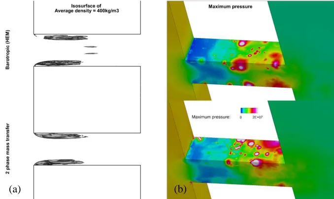
Simulation with the LES CSM model, under the configuration outlined above, gives an average mass flow rate of 7.23g/s for the 2 phase model and 7.27g/s for the barotropic model, whereas the experimental flow rate is 7.3g/s. In fig. 3a the average distribution of vapor fraction is shown and in fig. 3b the maximum pressure recorded on the wall of the channel. As can be seen from the results, a similar pattern is found from the two cavitation models both in terms of average density distribution and maximum wall pressure. It has to be highlighted that with the tuning of the mass transfer
coefficients the minimum pressure in the two phase model is -3bar; if no tuning was used, then the minimum pressure is of the order of -20bar.
Fig. 2. (a) Average density inside the throttle, indicated with an isosurface at 400kg/m3 (b) Maximum pressure distribution on the throttle wall, pressures may exceed 500bar in white zones.
4. Conclusion
In this paper, the performance of two cavitation models has been analyzed in a fundamental shock tube case and in a throttle case. From the shock tube case, it is evident that both the barotropic and the two phase cavitation models are equivalent, provided that the mass transfer of the latter is high enough to tend towards thermodynamic equilibrium. The throttle case confirms this finding, since both models show a similar cavitation zone, while also predict pressure peaks indicating the collapse of cavitation structures.
References
[1] Dular M and Coutier-Delgosha O 2009 Numerical modelling of cavitation erosion. Int J Numer
Methods Fluids, 61: p. 1388-1410.
[2] Goncalves E and Patella R F 2009 Numerical simulation of cavitating flows with homogeneous models. Computers & Fluids, 38: p. 1682–1696.
[3] Egerer C, et al. 2014 Large-eddy simulation of turbulent cavitating flow in a micro channel. Phys
Fluids, 26: p. 30.
[4] Pelanti M and Shyue K-M 2014 A mixture-energy-consistent six-equation two-phase numerical model for fluids with interfaces, cavitation and evaporation waves. J Comput Phys, 259: p. 331-357.
[5] Gavaises M, et al. 2015 Visualisation and les simulation of cavitation cloud formation and collapse in an axisymmetric geometry. Int J Multiphase Flow, 68: p. 14-26.
[6] ANSYS 2013 ANSYS Fluent 15.07.
[7] Brennen C 1995 Cavitation and Bubble Dynamics. (Oxford University Press).
[8] Kobayashi H and Wu X 2006 Application of a local subgrid model based on coherent structures to complex geometries, Center for Turbulence Research. p. 69-77.
[9] Edelbauer W, Strucl J, and Morozov A 2014 Large Eddy Simulation of cavitating throttle flow, in
SimHydro 2014:Modelling of rapid transitory flows (Sophia Antipolis).
[10] Perkovic I, et al. 2008 3D CFD Calculation of Injector Nozzle Model Flow for Standard and Alternative Fuels, in HEAT 2008, Fifth International Conference on Transport Phenomena In
Multiphase Systems (Bialystock, Poland).
(a) (b)
9th International Symposium on Cavitation (CAV2015) IOP Publishing Journal of Physics: Conference Series 656 (2015) 012086 doi:10.1088/1742-6596/656/1/012086
[image:5.595.129.468.138.340.2]