City, University of London Institutional Repository
Citation
:
He, Y., Jejjala, V., Matti, C., Nelson, B. D. & Stillman, M. (2015). The Geometry of Generations. Communications in Mathematical Physics, 339(1), pp. 149-190. doi:10.1007/s00220-015-2416-7
This is the accepted version of the paper.
This version of the publication may differ from the final published
version.
Permanent repository link: http://openaccess.city.ac.uk/12861/
Link to published version
:
http://dx.doi.org/10.1007/s00220-015-2416-7Copyright and reuse:
City Research Online aims to make research
outputs of City, University of London available to a wider audience.
Copyright and Moral Rights remain with the author(s) and/or copyright
holders. URLs from City Research Online may be freely distributed and
linked to.
WITS-CTP-143
The Geometry of Generations
Yang-Hui He,a,b,c Vishnu Jejjala,d Cyril Matti,a Brent D. Nelson,e,f Michael Stillmang
aDepartment of Mathematics, City University, London, EC1V 0HB, UK
bSchool of Physics, NanKai University, Tianjin, 300071, P.R. China
cMerton College, University of Oxford, OX1 4JD, UK
dCentre for Theoretical Physics, NITheP, and School of Physics, University of the Witwatersrand,
Johannesburg, WITS 2050, South Africa
eDepartment of Physics, Northeastern University, Boston, MA 02115, USA
fICTP, Strada Costiera 11, Trieste 34014, Italy
gDepartment of Mathematics, Cornell University, Ithaca, NY 14853-4201, USA
E-mail: hey@maths.ox.ac.uk,vishnu@neo.phys.wits.ac.za,
cyril.matti.1@city.ac.uk,b.nelson@neu.edu,mike@math.cornell.edu
Abstract: We present an intriguing and precise interplay between algebraic geometry and the phenomenology of generations of particles. Using the electroweak sector of the MSSM as a testing ground, we compute the moduli space of vacua as an algebraic variety for multiple generations of Standard Model matter and Higgs doublets. The space is shown to have Calabi–Yau, Grassmannian, and toric signatures which sensitively depend on the number of generations of leptons, as well as inclusion of Majorana mass terms for right-handed neutrinos. We speculate as to why three generations is special.
Contents
1 Introduction 2
2 MSSM Vacuum Moduli Space 3
2.1 F-terms and D-terms 3
2.2 Computational Algorithm 5
3 Multi-generation Electroweak Models 6
3.1 Relations, Syzygies, and Grassmannian 8
3.2 Counting Operators with Hilbert Series 11
3.3 Vacuum Geometry 11
4 Multiple Higgs Generations 18
5 Right-handed Neutrinos 20
5.1 Vacuum Geometry 23
5.2 Role of the Majorana Mass Term 27
5.3 Vacuum Geometry: GeneralNf 31
6 Discussion and Outlook 34
A Gauge Invariant Operators in the MSSM 37
B Toric Varieties 38
C Affine Calabi–Yau Toric Varieties 41
1 Introduction
The Standard Model of particle physics is an incomplete theory of the gauge interactions. We expect that the physics which extends the Standard Model at energies above 1–10 TeV invokes supersymmetry and derives from some higher energy theory that also incorporates gravity. A key property of any quantum field theory is its vacuum and in the context of supersymmetric gauge theories, the vacuum possesses interesting structure. This is because the supersymmetric vacuum is the solution of F-flatness and D-flatness conditions. Generi-cally, this is a continuous manifold parametrized by the gauge invariant operators (GIOs) of the theory. Importantly, this vacuum moduli space is an algebraic variety, which can have intricate geometric properties. The topology and algebraic geometry of the vacuum is coex-tensive with phenomenology [1,2]. Exploring the structure of the vacuum therefore provides a low energy window into deducing how certain theories of phenomenological interest can both encode and be guided by interesting geometry.
The most na¨ıve extension of known particle physics is the MSSM, which expands the Higgs sector of the theory by introducing separate SU(2)L doublets for up-type quark and down-type quark Yukawa couplings. The vacuum geometry of this theory, or related theories like the NMSSM, is not known, even though it has existed as a computational challenge to the community for many decades [3–7]. This is because the vacuum moduli spaces of N = 1 theories are expressed as relations between the generators of the GIOs, which are monomials in the superfields of the theory. The minimal list contains 991 generators for GIOs in the MSSM [3]. These are not fully independent and are related by the 49 F-term equations for the component matter superfields in the theory. Although this effort motivated [1,2], solving for the vacuum of the full MSSM was then beyond our reach.
While the exact vacuum geometry remains unknown, we can ask and hope to answer a different class of questions. We know, for instance, that for generic numbers of flavorsNf and colors Nc, the vacuum moduli space of supersymmetric QCD is a Calabi–Yau manifold [8]. Does this property extend to the vacuum geometry of the MSSM? Is there something special, geometrically speaking, about the particle content that we see experimentally? Why are there three generations of matter fields at low energies? It is difficult to imagine questions that are more pressing, especially from the point of view of string theory, which purports to be a fundamental theory. In this case, the initial conditions that describe the Standard Model are, in fact, the result of some vacuum selection principle.
is in some sense orthogonal to the traditional techniques of gauge invariance and discrete symmetries. A first attempt to define what such a program might look like is given in [1,2]. Since that time, advances in computational algebraic geometry software, as well as overall advances in computation, have allowed us to probe further than could have been conceived eight years ago. The first paper to re-address this fundamental problem appeared recently [9]. The current article seeks to build on these advances to explore the electroweak sector of the MSSM in the broadest possible context. Fortified by the discovery of interesting geometry encoded in the vacuum moduli space of the MSSM, we wish to find out whether geometry can say anything new about the nature of generations of particles. Intriguingly, it does.
The paper is organized as follows. In Section 2, we review how to compute the vacuum moduli space of a supersymmetric theory. This allows us to set notation and establish our conventions. In Section 3 we present results obtained from considering a minimal renor-malizable superpotential and various numbers of particle flavors. We explicitly describe the vacuum geometry for the casesNf = 2,3,4,5. In Section4, we consider multiple generations of Higgs fields for this minimal superpotential. In Section 5, we then move on to theories with right-handed neutrinos fields with Majorana mass terms and then without. We give the vacuum geometry for the cases Nf = 2,3,4, as well as a general description for general
Nf in the case without Majorana mass terms. We conclude in Section 6. Appendices A, B andCcontain complementary information about the full MSSM GIO content and about the method used to obtain toric diagrams from binomial ideals.
2 MSSM Vacuum Moduli Space
We begin by reminding the reader of the algorithm with which we explicitly calculate the vacuum moduli space of supersymmetric gauge theories from the point of view of computa-tional algebraic geometry, focusing on the MSSM. First, we introduce the matter content and the superpotential and then we summarize the algorithm.
2.1 F-terms and D-terms
In order to set the scene and specify our notation, let us briefly review the context of four-dimensional supersymmetric gauge theories and the Minimal Supersymmetric Standard Model (MSSM) field content.
A generalN = 1 globally supersymmetric action in four dimensions is given by
S=
Z
d4x
Z
d4θ Φ†ieVΦi+
1 4g2
Z
d2θ trWαWα+
Z
d2θ W(Φ) + h.c.
where Φi are chiral superfields, V is a vector superfield,Wα are chiral spinor superfields, and the superpotentialW is a holomorphic function of the superfields Φi. Each of these objects transforms under the gauge groupGof the theory: Φi under some representation Ri and V in the Lie algebrag. The chiral spinor superfields are the gauge field strength and are given byWα=iD
2
e−VDαeV.
The vacuum of the theory consists of φi0, the vacuum expectation values of the scalar components of the superfields Φithat provide a simultaneous solution to the F-term equations
∂W(φ)
∂φi
φi=φi0
= 0 (2.2)
and the D-term equations
DA=X i
φ†i0TAφi0= 0, (2.3)
whereTAare generators of the gauge group in the adjoint representation, and we have chosen the Wess–Zumino gauge.
The MSSM fixes the gauge group G= SU(3)C ×SU(2)L×U(1)Y. We will adopt the notation given in Table1for the indices and the field content of the theory. For the moment, we do not consider right-handed neutrinos, which are gauge singlets.
INDICES
i, j, k, l= 1,2, . . . , Nf Flavor (family) indices
a, b, c, d= 1,2,3 SU(3)C color indices
α, β, γ, δ= 1,2 SU(2)L indices
FIELDS
Qi
a,α SU(2)L doublet quarks
uia SU(2)L singlet up-quarks
dia SU(2)L singlet down-quarks
Liα SU(2)Ldoublet leptons
ei SU(2)L singlet leptons
Hα up-type Higgs
[image:6.612.95.537.381.526.2]Hα down-type Higgs
Table 1. Indices and field content conventions for the MSSM.
The corresponding minimal renormalizable superpotential is
Wminimal = C0
X
α,β
HαHβαβ+
X
i,j
Cij1 X
α,β,a
Qia,αujaHβαβ
+X
i,j
Cij2 X
α,β,a
Qia,αdjaHβαβ+
X
i,j
Cij3eiX
α,β
LjαHβαβ , (2.4)
these terms respect R-parity. The problem of finding the vacuum moduli space of the theory thus reduces to solving (2.2) and (2.3) for the above superpotential.
2.2 Computational Algorithm
Algebraic geometry has proven a useful and powerful tool to tackle problems in gauge fields theories, not least the challenge of providing a mathematical description of vacuum moduli spaces [10]. The problem of solving (2.2) and (2.3) is equivalent to the elimination algorithm detailed below.
Let us denote the gauge invariant operators (GIOs) by rj({φi}). The full list of gen-erators for the MSSM GIOs is given in Appendix A.1 The description of the moduli space of N = 1 theories as the symplectic quotient of the space of F-flat field configurations by the complexified gauge groupGC is well known [4–7, 11]. Our goal is to provide an efficient methodology for implementing this result.
Let us consider the ideal
∂W ∂φi
, yj −rj({φi})
⊂R=C[φi=1,...,n, yj=1,...,k], (2.5)
whereyi are additional variables. Then, eliminating all variablesφi of this ideal will give an ideal in terms of the variablesyi in the polynomial ringS=C[yj=1,...,k] only. The result will be the vacuum moduli space as an algebraic variety inS. From the standpoint of algebraic geometry, the above prescription amounts to finding the image of a map from the quotient ring
F = C[φi=1,...,n]
h∂W∂φ
ii
(2.6)
to the ringS =C[yj=1,...,k].2 (See [12,13] for further details.) This algorithm can be summarized in the following way:
• INPUT:
1. Superpotential W({φi}), a polynomial in variables φi=1,...,n.
2. Generators of GIOs: rj({φi}), j= 1, . . . , k polynomials inφi.
• ALGORITHM:
1
This table was already presented in [2] and stems from earlier work of [3]. Here, we have corrected some
minor typographical errors with respect to the indices. 2
1. Define the polynomial ringR =C[φi=1,...,n, yj=1,...,k].
2. Consider the ideal I =h∂W
∂φi, yj−rj({φi})i.
3. Eliminate all variables φi from I ⊂R, giving the idealM in terms ofyj.
• OUTPUT:
M corresponds to the vacuum moduli space as an affine variety inC[y1, . . . , yk].
This paper focuses on discussing the output of this algorithm for the MSSM electroweak sector, considering various number of particle flavors. The resulting affine varieties M are intersections of homogeneous polynomials and, as such, we can write them as affine cones over a compact projective varietyBof one lower dimension. We will thus adopt the notation to which we have adhered for many years,
M= (k|d, δ|mn1 1 m
n2
2 . . .) := Affine variety of complex dimension d, realized as an affine cone over a projective variety of dimensiond−1 and degree δ,
given as the intersection ofni polynomials of degreemi inPk.
(2.7)
3 Multi-generation Electroweak Models
Presently, we contemplate a renewed effort to calculate the full geometry of the MSSM vac-uum moduli space. The computing power required for applying the previously described algorithm with ∼ 1000 GIOs and ∼50 fields is well beyond what is accessible by standard personal computers. The use of supercomputers is envisaged. For this reason, our goal here is significantly more modest, and we only unveil aspects of the geometry for the electroweak sector. That is, we study a subsector of the full vacuum moduli space that is given by the additional constraints that the vacuum expectation values of the quark fields vanish:
Qia,α=uia=dia= 0 . (3.1)
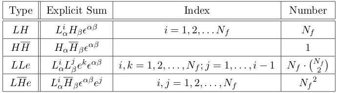
This is perhaps reasonable on phenomenological grounds asSU(3)C is an unbroken symmetry in Nature. The non-vanishing GIOs that remain from the list in Appendix A are noted in Table2.
The minimal renormalizable superpotential of the electroweak sector of the MSSM is then
Wminimal=C0HαHβαβ+
X
i,j
Type Explicit Sum Index Number
LH LiαHβαβ i= 1,2, . . . Nf Nf
HH HαHβαβ 1
LLe LiαLjβekαβ i, k= 1,2, . . . , Nf;j= 1, . . . , i−1 Nf · N2f
[image:9.612.133.480.78.173.2]
LHe LiαHβαβej i, j= 1,2, . . . , Nf Nf2
Table 2. Minimal generating set of the GIOs for the electroweak sector.
Henceforth, we are explicit about the sums on flavor indices i, j but leave sums on SU(2)L indicesα, β implicit. The corresponding F-terms are
∂Wminimal
∂Hα
=C0Hβαβ , (3.3)
∂Wminimal
∂Hβ
=C0Hααβ +
X
i,j
Cij3eiLjααβ , (3.4)
∂Wminimal
∂Ljα
=X
i
Cij3eiHβαβ , (3.5)
∂Wminimal
∂ei =
X
j
Cij3LjαHβαβ . (3.6)
In particular, this yields the following F-term equations for the Higgs fields:
Hβ = 0, (3.7)
C0Hα+
X
i,j
Cij3eiLjα= 0, (3.8)
from theFHα andFHβ terms, respectively. The other two F-term equations (for the eandL fields) do not lead to extra constraints as the vanishing ofHβ renders them trivial.
In terms of the{ri}, the only non-trivial GIOs that remain are theLHandLLeoperators. Indeed, HH and LHevanishes by virtue of (3.7). Furthermore, (3.8) specifies the value of theLH operators in terms of the LLe operators. Multiplying (3.8) by Li
βαβ and summing onα gives
C0LiαHβαβ+
X
j,k
Cjk3 LiαLjβekαβ = 0. (3.9)
(We have takenCij3 =Cji3.) Since there is a free indexiin (3.9), there areNf linear equations which suppress the LH variables as degrees of freedom in the vacuum moduli space. Thus, onlyLLecontributes to the dimension counting of the vacuum geometry and the moduli space reduces to an affine variety in C[y1, . . . , yk] with k= 1, . . . , Nf · N2f
among theLLepolynomials.3 The remaining coordinatesy resulting from theLH operators only provide an embedding into the bigger ringC[y1, . . . , yk+Nf].
3.1 Relations, Syzygies, and Grassmannian
Having established that the moduli space is only given by the relations among theLLe oper-ators, let us study these relations4 explicitly for some specified number of matter generations
Nf. Explicitly, LLe = LiαL j
βekαβ. The flavor index k of the electron can assume any of the Nf possibilities. The indices i and j must be different due to the contraction with the antisymmetric tensor. There are therefore Nf
2
choices for the combination Li αL
j
βαβ. Be-cause theSU(2)L indices α, β only take values 1,2, there is an upper bound on the number of lepton doublets that we can introduce before certain composite operators perforce vanish. Indeed, there are relations between combinations of LLeoperators. Taking into account ev-ery possible index combination with (i, j) 6= (m, n) and k6= p, a bit of algebra allows us to deduce the relation
(LiαLjβekαβ)(LmγLnδepγδ) = (LmαLnβekαβ)(LiγLjδepγδ) . (3.10)
These are the relations for the ideal, which we write as
h (LiαLjβekαβ)(LmαLnβepαβ)−(LmαLnβekαβ)(LiαLjβepαβ)i. (3.11)
In a slight abuse of convention, we have restricted the remit of sums over SU(2)L indices to lie within the parentheses when we write out operators withLL fields explicitly. We will adopt this convention from now on.
Heuristically, given the form of the relations in the ideal, we can cast the defining relations as an equality of quotients:
LiαLjβekαβ
Li αL
j βepαβ
= L m
αLnβekαβ
Lm
αLnβepαβ
, (3.12)
where again the summation over α, β restricts to the numerator or the denominator. The equality (3.12) informs us that a set of operators with a common ek field will be linearly proportional to another set of operators with a commonep field (k 6=p). In a strict math-ematical sense, (3.12) only applies when the operators are non-vanishing in order to avoid problems with divisions by zero. Nevertheless, this notation is a convenient way to succinctly
3By abuse of terminology, we identify the ring
C[y1, . . . , yk] and its corresponding k-affine spaceCk, whereby
not making the distinction between the two, as is customary in the physics community. 4
The relations are presented in [3]; however, here we add to that analysis by presenting and counting the
express the relations we have encountered, keeping in mind that the branches with vanishing operators must be taken into account as well.
To determine the dimension of the variety, we only need to count a minimal generating set of such equations. There are (Nf −1)
Nf 2
−1non-trivial constraints when Nf ≥3.
When Nf ≥4, more relations occur from the LL component of the LLe operators. We have
(LiαLjβαβ)(LkαLlβαβ) + (LiαLkβαβ)(LlαLjβαβ) + (LiαLlβαβ)(LjαLkβαβ) = 0. (3.13)
The set of indicesi, j, k, lcan be chosen, without loss of generality, to be in a strictly increasing order. This implies that there are Nf
4
such relations. Let us introduce
Pijkl := (LiαLjβαβ)(LkαLlβαβ),
Pi(jkl) := X
cyclic permutations (jkl)
Pijkl. (3.14)
We can then readily write (3.13) in the compact form:
Pi(jkl)= 0. (3.15)
In general, this set of equations will be highly redundant as syzygies (relations among the generators) begin to appear. Among the polynomialsP, we have the syzygies
Pi(jkl)(LiαLmβαβ)−Pi(jkm)(LiαLlβαβ) +Pi(jlm)(LiαLkβαβ) = Pi(klm)(LiαLjβαβ),(3.16)
Pi(jkl)(LjαLmβαβ)−Pi(jkm)(LjαLlβαβ) +Pi(jlm)(LjαLkβαβ) = Pj(klm)(LiαLjβαβ).(3.17)
These syzygies imply that the relations (3.15) can be chosen such that the indicesi= 1 andj= 2 without loss of generality. Indeed, all other choices of indices are simply redundant equations. To see this, we can use the first syzygy (3.16) to generate allPs starting with an indexi= 1 fromPs starting with an indexi= 1 andj= 2. Explicitly, with the conventions that indices are in a strictly increasing order, we observe that all P1(klm) fork, l, m > 2 are given by the relation
P1(2kl)(L1αLmβαβ)−P1(2km)(L1αLlβαβ) +P1(2lm)(L1αLkβαβ) =P1(klm)(L1αL2βαβ). (3.18)
Having established that we can generate every polynomial P starting with an index 1, we can use the second syzygy (3.17) with a choice of index i= 1 and any indices m > l > k > j ≥ 3 to show that every relation in (3.15) with indices (i, j, k, l) greater than 2 are redundant:
We can now count the total number of independent relations:
# relations =
Nf −2 2
. (3.20)
This is due to the fact that the independent constraints in (3.15) are given by P1(2kl) = 0 only. So we need to choose two indices (kand l) amongNf −2 possibilities (i= 1 and j= 2 being fixed).
Taking all of the above counting together, the dimension of the vacuum moduli space will be
Nf ·
Nf 2
−(Nf −1)
Nf 2
−1
−
Nf−2 2
= 3Nf −4. (3.21)
The vacuum geometry can be understood as follows. Explicitly, the index structure
LLe= LiαLjβekαβ shows that LiαLjβαβ furnishes, due to the antisymmetry, coordinates on the GrassmannianGr(Nf,2) of two-planes inCNf. The freely indexedek, on the other hand, gives simply a copy ofPNf−1. Topologically, the geometry is then given by (the affine cone
over)Gr(Nf,2)×PNf−1.
In fact, the above dimension counting simply corresponds to the dimension of the Grass-mannian
dimGr(n, r) =r(n−r), (3.22)
given by theLLpart of the operators. Therefore, according to the productGr(Nf,2)×PNf−1,
the affine dimension is obtained
dimMEW = 2(Nf −2) +Nf = 3Nf−4. (3.23)
Thus, the dimension always increases by three when we add another generation of matter fields to the electroweak sector.
It is a remarkable fact that the dimension increases by the same increment as the number of fields, despite the number of GIOs growing much faster.
Nf 1 2 3 4 5 6 . . .
number of fields 5 8 11 14 17 21 . . .
number ofLLegenerators 0 2 9 24 50 90 . . .
vacuum dimension 0 2 5 8 11 14 . . .
Table 3. Vacuum geometry dimension according to the number generationsNf.
In the following subsections, we will study in greater detail the geometry for the cases
3.2 Counting Operators with Hilbert Series
The Hilbert series provides technology for enumerating GIOs in a supersymmetric quantum field theory. For a varietyM ⊂C[y1, . . . , yk], the Hilbert series supplies a generating function:
H(t) = ∞
X
n=−∞
dimMntn= P(t)
(1−t)d . (3.24)
This has a geometrical interpretation. The quantity dimMn that appears in the sum con-stitutes the (complex) dimension of the graded pieces ofM. That is to say, it represents the number of independent polynomials of degreenonM. When we write the Hilbert series as a ratio of polynomials, the numerator and the denominator both have integer coefficients. The dimension of the moduli space isd, which is the order of the pole att= 1. Via the plethystic exponential and the plethystic logarithm, the Hilbert series encodes information about the chiral ring and geometric features of the singularity from which the supersymmetric gauge theory under consideration arises. It should be emphasized that the Hilbert series is not a topological invariant and can be represented in many ways. For our purposes, an important caveat is that Hilbert series depends on the embedding of the variety within the polynomial ring [14]. The reader is referred to [15] for an account of the importance of the Hilbert series in the context of gauge theories.
In this investigation, we will write the Hilbert series for the vacuum moduli space of the electroweak sector for various values ofNf. The Hilbert series is a mathematical object that can be constructed using standard techniques in computational algebraic geometry. Knowl-edge of certain properties of the Hilbert series will allow us to characterize the structure of the vacuum geometry.
3.3 Vacuum Geometry
Let us introduce the following label for the non-vanishingLLeoperators
yI+C(Nf,2)·(k−1)=L i αL
j βe
kαβ , (3.25)
where C(Nf,2) = N2f
are binomial coefficients and I = 1, . . . , C(Nf,2) accounts for the (i, j) index combinations from LiαLjβαβ. With this notation, the first set of relations (3.12) becomes,
yI+C(Nf,2)·(k−1)
yI+C(Nf,2)·(l−1)
= yJ+C(Nf,2)·(k−1)
yJ+C(Nf,2)·(l−1)
, (3.26)
among each yI+C(Nf,2)·(k−1) for a fixed k when Nf is large enough (Nf ≥ 4). We cannot write these relations explicitly for all of theNf at once, so let us consider each value ofNf separately.5
Nf = 2
In this case, we have only twoLLeoperators for the two ei fields. Thus, we cannot have any relations and the vacuum moduli space is trivially the planeM=C2.
Nf = 3
We have nineLLeoperators and the vacuum moduli space will be an algebraic variety inC9.
With the above notation (3.25), the relations (3.26) become
y1
y4 = y2
y5 = y3
y6
, (3.27)
y1
y7 = y2
y8 = y3
y9
. (3.28)
This leads to an ideal given by nine quadratic polynomials
h y1y5−y2y4, y1y6−y3y4, y2y6−y3y5,
y1y8−y2y7, y1y9−y3y7, y2y9−y3y8, (3.29)
y4y8−y5y7, y4y9−y6y7, y5y9−y6y8 i .
We count (3−1) 32
−1
= 4 equalities in (3.27) and (3.28) and we find that the resulting moduli spaceMis an irreducible five-dimensional affine variety given by an affine cone over a base manifoldBof dimension four. As a projective variety, B has degree six and is described by the (non-complete) intersection of nine quadratics in P8, which agrees with the results
of [2,9]. This can be summarized according to the standard notation (2.7) as
MEW= (8|5,6|29). (3.30)
The variety M is in fact a non-compact toric Calabi–Yau. The reader is referred to AppendixC for a detailed discussion on toric affine Calabi–Yau spaces. Indeed, its Hilbert series is given by
1 + 4t+t2
(1−t)5 , (3.31)
and ispalindromic. By this, we mean simply that the numerator of the Hilbert series can be written in the form
P(t) = N
X
k=0
aktk, (3.32)
5 We stopped this investigation atN
with the simple property that ak = aN−k. It has been shown [16] that the numerator of the Hilbert series of a graded Cohen–Macaulay domain X is palindromic if and only if X
is Gorenstein6. For affine varieties, the Gorenstein property implies that the geometry is Calabi–Yau. Additional discussion of this point can be found in [8], and in Appendix C for clarifications on the Gorenstein property. The vacuum moduli spaces we obtain are non-compact.
As mentioned in Section 3.1, the topology is given by the cone overGr(3,2)×P2. The GrassmannianGr(3,2) is exactly P2, while the secondP2 comes fromPNf−1. Therefore, the
affine five-dimensional vacuum space described by (3.30) is none other than the cone over the Segr`e embedding of P2 ×P2 into P8. We remind the reader that this is the following
space. Take [x0 : x1 :x2] and [z0 : z1 : z2] as the homogeneous coordinates on the two P2s
respectively and consider the quadratic map
P2 × P2 −→ P8
[x0 :x1 :x2] [z0:z1 :z2] → xizj
, (3.33)
where i, j = 0,1,2 give precisely the 32 = 9 homogeneous coordinates of P8. Explicitly,
upon elimination, this is exactly the nine quadrics with the Hilbert series as given in (3.30) and (3.31). We also point out that this Segr`e variety is the only Severi variety of projective dimension four. Later we will re-encounter Severi varieties of a unique nature in dimension two.
For the reader’s convenience, let us recall the definition of a Severi variety [17–19].7 It is a classic result of Hartshorne–Zak [18] that any smooth non-degenerate algebraic variety
X of (complex) dimension n embedded intoPm with m < 32n+ 2 has the property that its
secant varietySec(X) —i.e., the union of all the secant and tangent lines toX — is equal toPm itself. The limiting case8 ofm= 32n+ 2 andSec(X)6=Pn is called aSeveri variety. The classification theorem of Zak [18] states that there are only four Severi varieties (the dimensions are precisely equal to 2q with q the dimension of the four division algebras):
n= 2: The Veronese surfaceP2 ,→P5;
n= 4: The Segr`e variety P2×P2,→P8;
6 In this work, for all the varieties considered, M is always an integral domain arithmetically Cohen–
Macaulay. Hence, we will loosely use the correspondence that, for affine varieties, palindromic Hilbert series
means Calabi–Yau. 7
We are grateful to Sheldon Katz for his insight and for mentioning Severi varieties to us. 8
n= 8: The GrassmannianGr(6,2) of two-planes in C6, embedded into P14;
n = 16: The Cartan variety of the orbit of the highest weight vector of a certain non-trivial representation of E6.
Of these, only two are isomorphic to (a product of) projective space, namely n = 2,4. Remarkably, these are the two that show up as the vacuum geometry of the electroweak sector whenNf = 3.
The connection with Severi varieties could be profound. Indeed, it was discussed in [19] that these four spaces are fundamental to mathematics in the following way. It is well-known that there are four division algebras: the real numbersR, the complex numbersC, the
quater-nionsH, and the octonionsO, of, respectively, real dimension 1,2,4,8. Consider the projective
planes formed out of them, viz., RP2, CP2, HP2 and OP2, of real dimension 2,4,8,16. We
have, of course, encountered CP2 repeatedly in our above discussions. The complexification
of these four spaces, of complex dimension 2,4,8,16 are precisely homeomorphic to the four Severi varieties. Amazingly, they are also homogeneous spaces, being quotients of Lie groups. In summary, we can tabulate the four Severi varieties
Projective Planes Severi Varieties Homogeneous Spaces
RP2 CP2 SU(3)/S( U(1)×U(2) ) CP2 CP2×CP2 SU(3)2/S( U(1)×U(2) )2 HP2 Gr(6,2) SU(6)/S( U(2)×U(4) ) OP2 S E6/Spin(10)U(1)
(3.34)
Returning to our present case ofn= 4, the embedding (3.33) can be understood in terms of the previously definedy variables. Let us consider the following change of variables,
y1 →z0x2 , y2 →z0x1 , y3 →z0x0 ,
y4 →z1x2 , y5 →z1x1 , y6 →z1x0 ,
y7 →z2x2 , y8 →z2x1 , y9 →z2x0 .
(3.35)
Thez coordinates labels the C3 due to theefields, while the x coordinates label the
Grass-mannian due toLL. With these variables, the relations (3.27) and (3.28) are automatically satisfied.
ideal (3.29). Its toric diagram can be presented as follows, N=
1 0 1 0 0 1 1 0 0 0 1 1 0 1 0 0 0 1 0 0 0 1 0 0 0 0 1 0 1 0 0 −1 1 −1 1 0 0 0 −1 1 0 0 0 0 1
, (3.36)
where each row of the matrix corresponds to the vectors generating the toric cone. They are five-dimensional vectors as required for a five-dimensional variety. We have nine of them, as expected from the nine quadratics in (3.29). Further details on the toric diagrams are given in AppendixB.
Finally, we found that the Hodge diamond of the base space Bis given by
hp,q(B) =
h0,0
h0,1 h0,1
h0,2 h1,1 h0,2
h0,3 h1,2 h1,2 h0,3
h0,4 h1,3 h2,2 h1,3 h0,4
h0,3 h1,2 h1,2 h0,3
h0,2 h1,1 h0,2
h0,1 h0,1
h0,0
=
1 0 0
0 2 0
0 0 0 0
0 0 3 0 0
0 0 0 0
0 2 0
0 0 1
, (3.37)
which has the peculiar property to be non-vanishing in its diagonal only. This Hodge diamond is consistent with the Hodge diamond ofP2×P2 as can be seen by using the K¨unneth formula.
Of course, as is with a later example in (5.58), having the same Hodge diamond is only a statement of topology, our analysis is more refined in that we can identify what the variety actually is.
We note that the surface itself was first identified in [2], but the only information that could be gleaned about the manifold at that time is that encapsulated by the notation of (3.30).9 Since that time, improvements in computing and software have allowed us to calculate both the Hilbert series and the above Hodge diamond, as well as leading to a com-plete understanding of its geometrical nature.
Nf = 4
For the case of four flavors, we have twenty-four LLe operators. The first set of con-straints (3.26) leads to (4−1) 42
−1
= 15 equations. With the notation defined in (3.26) and the simplified choice ofLLlabeling, we have
y1
y7 = y2
y8 = y3
y9 = y4
y10 = y5
y11 = y6
y12
, (3.38)
y1
y13 = y2
y14 = y3
y15 = y4
y16 = y5
y17 = y6
y18
, (3.39)
y1
y19 = y2
y20 = y3
y21 = y4
y22 = y5
y23 = y6
y24
. (3.40)
Moreover, we need to take care of the constraints from the second set of relations (3.15). Due to the fact that we only have six possibleLL operators, we will have only one relation among them, given by
(L1αL2βαβ)(L3αL4βαβ)−(L1αL3βαβ)(L2αL4βαβ) + (L1αLβ4αβ)(L2αL3βαβ) = 0. (3.41)
We can multiply this relation with anyefield to obtain the relations among LLe operators, translated into they variable. Fore1, we have,
y1y6+y3y4−y2y5= 0, (3.42)
while for the other threeefields, we have,
y7y12+y9y10−y8y11= 0,
y13y18+y15y16−y14y17= 0,
y18y24+y21y22−y20y23= 0. (3.43)
It is straightforward to see that these equations do not lead to additional constraints. Indeed, using (3.38)–(3.40) we can easily recover these from (3.42). Therefore, we have in total 4−22
= 1 relation as expected. The dimension of the vacuum moduli space is therefore 24−15−1 = 8. In fact, we have an irreducible eight-dimensional algebraic variety given by
M= (23|8,70|2100). (3.44)
In general, forNf >3, the Grassmannian does not degenerate to projective space though the geometry still corresponds to some embedding of Gr(Nf,2)×PNf−1 into higher
The embedding could again be understood from a change of variables. Writing the Pl¨ucker coordinate for Gr(4,2) as [x0 :x1 :x2 :x3 :x4 :x5] and taking [z0 :z1 :z2 :z3] for
P3, we can consider the change of variables,
y1 →z0x0 , y2 →z0x1 , y3 →z0x2 , y4 →z0x3 , y5 →z0x4 , y6 →z0x5 ,
y7 →z1x0 , y8 →z1x1 , y9 →z1x2 , y10→z1x3 , y11→z1x4 , y12→z1x5 ,
y13→z2x0 , y14→z2x1 , y15→z2x2 , y16→z2x3 , y17→z2x4 , y18→z2x5 ,
y19→z3x0 , y20→z3x1 , y21→z3x2 , y22→z3x3 , y23→z3x4 , y24→z3x5 .
(3.45)
Imposing the Pl¨ucker relation
x0x5−x1x4+x2x3 = 0 , (3.46)
for the coordinates [x0:x1:x2:x3 :x4 :x5], all required relations are then satisfied. Using algebraic geometry packages [20,21], we obtain the Hilbert series
1 + 16t+ 36t2+ 16t3+t4
(1−t)8 . (3.47)
Noting the palindromic property of the numerator, again we have an affine Calabi–Yau geom-etry. However, the additional condition (3.42) is not explicitly toric. We have this remarkable fact that only three generations of particles will provide explicitly toric geometries. Indeed, any number above three will have relations such as the one above.
Nf = 5
To illustrate the syzygies, let us look at the case withNf = 5. There are 50LLe operators. The relations (3.12) therefore contain 36 equalities:
y1
y11 = y2
y12 = y3
y13 = y4
y14 = y5
y15 = y6
y16 = y6
y17 = y7
y18 = y8
y19 = y10
y20
,
y1
y21 = y2
y22 = y3
y23 = y4
y24 = y5
y25 = y6
y26 = y6
y27 = y7
y28 = y8
y29 = y10
y30
,
y1
y31 = y2
y32 = y3
y33 = y4
y34 = y5
y35 = y6
y36 = y6
y37 = y7
y38 = y8
y39 = y10
y40
,
y1
y41 = y2
y42 = y3
y43 = y4
y44 = y5
y45 = y6
y46 = y6
y47 = y7
y48 = y8
y49 = y10
y50
. (3.48)
The relations obtained from (3.15) lead to the 54
= 5 equations:
y1y6+y3y4−y2y5= 0, (3.49)
y1y9+y3y7−y2y8= 0, (3.50)
y1y10+y5y7−y4y8= 0, (3.51)
y2y10+y6y7−y4y9= 0, (3.52)
The other relations forei withi6= 1 will not bring additional constraints due to the first set of relations (3.12). Now, we claimed that only the 5−22
= 3 relations from P1(2kl) = 0 are relevant. Indeed, we can multiply (3.49), (3.50), and (3.51) by the appropriate y variable to obtain
y2(y1y10+y5y7−y4y8) + (y1y6+y3y4−y2y5)y7−y4(y1y9+y3y7−y2y8) =
y1(y2y10+y6y7−y4y9) = 0 (3.54)
yielding (3.52) and
y3(y1y10+y5y7−y4y8) + (y1y6+y3y4−y2y5)y8−y5(y1y9+y3y7−y2y8) =
y1(y3y10+y6y8−y5y9) = 0 (3.55)
yielding (3.53). Thus we only have three genuine relations and the dimension of the space is 50−36−3 = 11 as expected from (3.21).
Using algebraic geometry packages [20, 21], we found an irreducible algebraic variety given by
M= (49|11,1050|2525). (3.56)
Its Hilbert series is
1 + 39t+ 255t2+ 460t3+ 255t4+ 39t5+t6
(1−t)11 , (3.57)
and again, we have an affine Calabi–Yau space which is not itself an explicit toric variety.
4 Multiple Higgs Generations
Before considering the vacuum geometry of the MSSM electroweak sector in the presence of neutrinos, let us first stop to consider what effect changing the number of generations of Higgs multiplets might have on the results we have already obtained. Let Nh denote the number of pairs of Higgs doublets in the theory, and let us restrict ourselves to the case in whichNh ≤Nf. Both the up-type Higgs doublet Hαk and down-type Higgs doubletH
k α must now be labeled by a generation indexk= 1, . . . , Nh. The Yukawa coupling matrixC3 is now promoted to a three-index tensor Cij,k3 , where i, j = 1, . . . , Nf and k = 1, . . . , Nh, and we imagine a bilinear term that allows arbitrary mixing among the Higgs generations: C0
ij, with indicesi, j= 1, . . . , Nh. The range of the indices should be clear from the context and, from now on, we will leave the range implicit. The GIOs here are summarized in Table4.
Type Explicit Sum Index Number
LH LiαHβjαβ i= 1, . . . , Nf;j= 1, . . . , Nh Nf ·Nh
HH HαiHjβαβ i, j= 1, . . . , Nh Nh2
LLe LiαLjβekαβ i, k= 1, . . . , Nf;j= 1, . . . , i−1 Nf · N2f
HHe HiαHjβekαβ i= 1, . . . , Nh;j = 1, . . . , i−1;k= 1, . . . , Nf Nf · N2h
[image:21.612.112.504.78.189.2]
LHe LiαHkβαβej i, j= 1, . . . , Nf;k= 1, . . . , Nh Nf2·Nh
Table 4. Minimal generating set of the GIOs for the electroweak sector, for number of Higgs doublets
Nh>1.
large rates forµ→eγ processes, etc.). But our interest here is to ask whether such a model,
a prioripossible, or even natural, from the point of view of an underlying string theory,10 has a geometry that is significantly different from that which arises in the one generation case.
When Nh 6= 1, we expect a larger set of GIOs and thus, at least na¨ıvely, we might expect the vacuum moduli space to be of larger dimension than the Nh = 1 case. Indeed, the operator types LH and LHe from Table 2 now represent Nf ·Nh objects, while the bilinearHH now representsNh2 terms. Since the lepton doubletL and the down-type Higgs
H have the same SU(2)L×U(1)Y quantum numbers, we can extend the list of GIOs in a straightforward manner. A new operator type in the electroweak sector is HHe. It is the analog of theLLeterm and, because of the implicit antisymmetric tensor, is allowed only in the case of multiple Higgs doublets.
The minimal superpotential we consider in this section is therefore
Wminimal =
X
i,j
Cij0HαiHjβαβ +X i,j,k
Cij,k3 eiLjαHkβαβ . (4.1)
10
For example, in the spirit of trinification, there are three generations of Higgs doublets in the ∆27
model [22,23], which embeds the Standard Model on the worldvolume of a single D3-brane. Three generations
The F-terms are modified from those of (3.3)–(3.6) to read
∂Wminimal
∂Hi α
=X
j
Cij0Hjβαβ , (4.2)
∂Wminimal
∂Hkβ
=X
i
Cik0Hαiαβ+X i,j
Cij,k3 eiLjααβ , (4.3)
∂Wminimal
∂Ljα
=X
i,k
Cij,k3 eiHkβαβ , (4.4)
∂Wminimal
∂ei =
X
j,k
Cij,k3 LjαHkβαβ . (4.5)
This leads to the following F-term equations for the Higgs fields:
Hjβ = 0, (4.6)
X
i
Cik0Hαi +X i,j
Cij,k3 eiLjα= 0. (4.7)
Once again, the vanishing of Hjβ leaves the other two F-term equations trivially satisfied. Note that (4.7) now representsNh separate constraint equations, labeled by the free indexk.
As before, the necessary vanishing of theNhfieldsH j
β in the vacuum ensures the vanishing ofHH,LHe, and the new operatorsHHein the vacuum. Similarly, we have a set of relations for theLH operators formed by contraction of (4.7) withLlβαβ. We obtain,
Cik0HαiLlβαβ+X i,j
Cij,k3 eiLjαLlβαβ = 0. (4.8)
These are Nf ·Nh linear equations (from the k and l free indices) which suppress the LH variables as degrees of freedom in the vacuum moduli space. Thus, once again, only LLe
contributes to the dimension counting of the vacuum geometry and the moduli space reduces to an affine variety inC[y1, . . . , yk] withk= 1, . . . , Nf· N2f
given by the relations among the
LLepolynomials. Therefore, we see that the vacuum moduli space is completely independent of the number of Higgs generations in the model. From this analysis, we can argue that the vacuum moduli space of the MSSM electroweak sector, without neutrinos, will be a non-compact Calabi–Yau for all values of Nh ≤ Nf. Despite our na¨ıve intuition, the dimension of the vacuum geometry is unchanged, though the addition of extra Higgs degrees of freedom allows for an embedding into the now larger polynomial ringC[y1, . . . , yk+Nf·Nh].
5 Right-handed Neutrinos
Neutrinos have mass. The mass can be generated by a coupling of a right-handed neutrinoν
U(1)Y, this means that the fieldν is itself a GIO. On physical grounds,νshould not appear by itself in a phenomenological superpotential as this would be a tadpole, which we can remove by a field redefinition. We may have composite operators involvingν, the simplest beingνiνj, which introduces Majorana mass terms to the Lagrangian.
When considering right-handed neutrino fields, we previously noticed that some of the dimensions of the vacuum moduli space geometry get lifted. The resulting geometry becomes a three-dimensional Veronese surface for the case of three generations of particles [1, 2, 9]. In this paper, we would like to consider cases with different number of particle families and understand the role of the GIOs for the structure of the vacuum geometry, focusing on the Majorana mass terms.
Let us consider the electroweak sector as described in the previous section with the addition of extra right-handed neutrinos fields as presented in Table5.
Type Explicit Sum Index Number
[image:23.612.197.521.493.591.2]ν νi i= 1,2, . . . , Nf Nf
Table 5. Right-handed neutrinos fields.
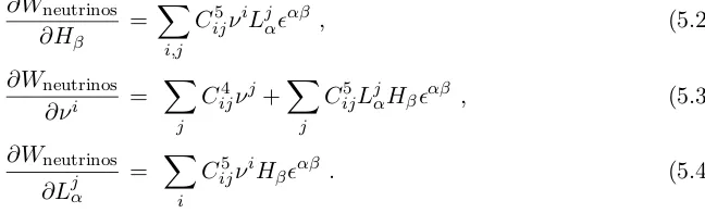
The corresponding superpotential terms are given by
Wneutrinos=
X
i,j
Cij4νiνj +X i,j
Cij5νiLjαHβαβ . (5.1)
Again, these interactions respect R-parity. Taking derivatives of the superpotential yields the F-terms:
∂Wneutrinos
∂Hβ
= X
i,j
Cij5νiLjααβ , (5.2)
∂Wneutrinos
∂νi =
X
j
Cij4νj +X j
Cij5LjαHβαβ , (5.3)
∂Wneutrinos
∂Ljα
= X
i
Cij5νiHβαβ . (5.4)
gives the full set of F-term equations:
X
i,j
Cij5νiLjααβ −C0Hααβ = 0, (5.5)
C0Hααβ +
X
i,j
Cij3eiLjααβ = 0, (5.6)
X
i
Cij5νiHβαβ+
X
i
Cij3eiHβαβ = 0, (5.7)
X
j
Cij4νj+X j
Cij5LjαHβαβ = 0, (5.8)
X
i
Cij3LjαHβαβ = 0. (5.9)
Recently in [9], it has been shown that this system of equations implies that the following GIOs vanish:
νi = 0, LH= 0, HH= 0, LHe= 0. (5.10)
Moreover, the only non-trivial equation remaining is (5.6). Contracting this condition with
Lkβ, we obtain:
X
i,j
Cij3eiLjαLkβαβ = 0. (5.11)
The vacuum geometry is therefore given by the relations and syzygies of the LLeoperators intersected with the hypersurface defined by (5.11).
For the sake of completeness, let us recall the demonstration from [9]. First, from (5.9) and from the non-singularity of the coupling matrix Cij3, we conclude that the GIOs LHe
must all vanish. Second, we contract (5.7) withLkα to obtain:
X
i
Cij5νiLkαHβαβ +
X
i
Cij3eiLkαHβαβ = 0. (5.12)
The second term vanishes by virtue ofLH = 0, and, assuming a generic matrixC5, we deduce
νiLkαHβαβ = 0. (5.13)
This implies that both νi and LH operators vanish. Indeed, if νi = 0, then6 LkαHβαβ = 0. From (5.8), we conclude thatνi= 0, in contradiction with the starting hypothesis. Therefore
5.1 Vacuum Geometry
Let us examine the geometries thus obtained. We start with the simple case of two flavors as an appetizer. Then we look at the famous Veronese solution and the corresponding higher-dimensional variety resulting from removing the Majorana mass terms. Then, we describe the corresponding vacuum geometry for the case of an additional flavor,Nf = 4.
Nf = 2
Let us first consider the case of two particle flavors as a warm up. We have seen that it has only two LLe operators coming from the two ei fields. Moreover, we now have two right-handed neutrino fields.
Considering the case without Majorana mass term, the system of equations (5.11) reduces to:
C113 e1L1αL2βαβ +C213 e2L1αL2βαβ = 0, (5.14)
C123 e2L1αL2βαβ+C223 e2L1αL2βαβ = 0. (5.15)
For the case when the coupling matrix C3 is a non-singular matrix, it is clear that the only solution to the above system is when LLe = 0. Thus the vacuum geometry consists of the point at the origin inC2.
Another way to write this ideal is to make the following change of variables:
˜
ej :=
X
i
Cij3ei. (5.16)
We subsequently definey variables in the same way as in Section 3:
y1= ˜e1L1αL2βαβ, y2= ˜e2L1αL2βαβ. (5.17)
Thus, the relations (5.14) immediately become
y1 = 0, y2= 0, (5.18)
and so we indeed have the point at the origin inC2 as the vacuum moduli space.
Nf = 3
To be complete, let us present again the defining polynomial ideal. Again, it is convenient to make the change of field variables:
˜
ej :=
X
i
Cij3ei , (5.19)
and define the followingy variables:
yI+C(Nf,2)·(k−1)= (−1)k−1LiαL j βe˜k
αβ . (5.20)
With this notation, the LLe˜relations retain a similar form to those we have found in Sec-tion3.2. In addition, we now have the relation (5.11) which corresponds to,
y1−y9 = 0, (5.21)
y2−y6 = 0, (5.22)
y4−y8 = 0. (5.23)
Thus, the full ideal is given by,
h y1y5−y2y4, y1y6−y3y4, y2y6−y3y5,
y1y8−y2y7, y1y9−y3y7, y2y9−y3y8, (5.24)
y4y8−y5y7, y4y9−y6y7, y5y9−y6y8,
y1−y9, y2−y6, y4−y8 i.
In fact, the last three linear terms can simply be used as constraints within the 9 quadrat-ics and, thus, reduce the ideal as a set of 6 quadratic polynomials. We have,
M= (5|3,4|26), (5.25)
and the corresponding Hilbert series,
1 + 3t
(1−t)3 . (5.26)
It should be noted that the Hilbert series is not palindromic and therefore the geometry is not Calabi–Yau.
The Veronese surface is an embedding ofP2intoP5. It is in fact the only Severi variety on
projective dimension two, and it is remarkable that two of the four Severi varieties appear as vacuum geometry for supersymmetric models with three flavor generations. The embedding is explicitly given by:
P2 → P5
[x0:x1:x2]7→ [x02:x0x1 :x12 :x0x2 :x1x2:x22]
This can again be understood in terms of the following change of variables:
y1→x0x2 , y2 →x0x1 , y3→x20 ,
y4→x1x2 , y5 →x21 , y6→x1x0 ,
y7→x22 , y8 →x2x1 , y9→x2x0 .
(5.28)
It should be observed that the effect of (5.11) is therefore to identify the two projective spaces arising from the Grassmannian Gr(3,2) and P2. Imposing the identification relation
[x0 : x1 : x2] = [z0 : z1 : z2] onto (3.33) lead to the vacuum geometry in the presence of right-handed neutrinos.
Again, we see from the binomial nature of the polynomial ideal (5.24) that the Veronese variety is toric. Using the same notation as previously, the corresponding diagram is given by,
N=
−1 −2 0
1 0 0
0 −1 0 1 0 −2 1 0 −1 0 −1 −1
=⇒ (5.29)
where we could include a pictorial representation of the toric cone, as it sits within three dimensions.
For the base space Bof the affine cone, we can compute its Hodge diamond
hp,q(B) =
h0,0
h0,1 h0,1
h0,2 h1,1 h0,2
h0,1 h0,1
h0,0
=
1 0 0
0 1 0
0 0 1
. (5.30)
Nf = 4
We give only the Hilbert series and dimension as writing the full ideal is tedious and ulti-mately unilluminating. However we realize that all the previous structures we have noted remain the same. The geometry stems out ofGr(4,2)×P3. As in the Veronese case, some identifications occur between the points inGr(4,2) andP3due to (5.11). With theyvariables
definition (5.20), these linear relations (5.11) become:
y1−y16+y23= 0, (5.31)
y2−y10+y24= 0, (5.32)
y3−y11+y18= 0, (5.33)
y7−y14+y21= 0. (5.34)
The identification is therefore not as straightforward as for the Veronese case, since we have a sum of three terms in each equality. In terms of theGr(4,2) and P3 variables, keeping the
same variables as defined by (3.45), these linear equations become
z0x0−z2x3+z3x4= 0, (5.35)
z0x1−z1x3+z3x5= 0, (5.36)
z0x2−z1x4+z2x5= 0, (5.37)
z1x0−z2x1+z3x2 = 0. (5.38)
The vacuum moduli space is therefore given by (3.45), subject to the constraints (3.46) and (5.35)–(5.38). It corresponds to a geometry of the type
M= (19|6,40|284) . (5.39)
It is irreducible, and its Hilbert series is
1 + 14t+ 21t2+ 4t3
(1−t)6 . (5.40)
5.2 Role of the Majorana Mass Term
It should be noted that key to the argument in the previous subsection is the fact that the
νi vanish due to equation (5.8). Now, when considering a superpotential without Majorana mass terms,e.g., with
C4 = 0,
this argument does not apply anymore. Instead, we have the following system for the F-term equations:
X
i,j
Cij5νiLjααβ −C0Hααβ = 0, (5.41)
C0Hααβ +
X
i,j
Cij3eiLjααβ = 0, (5.42)
X
i
Cij5νiHβαβ+
X
i
Cij3eiHβαβ = 0, (5.43)
X
j
Cij5LjαHβαβ = 0, (5.44)
X
i
Cij3LjαHβαβ = 0. (5.45)
From this, we can deduce again that allLH must vanish from (5.45). The difference is now that we can also deduce that all LH must vanish from (5.44). Finally, contracting (5.41) withHβ and with LH = 0, we also have that HH = 0. In summary, we have the following vanishing GIOs,
LH = 0, HH= 0, LHe= 0. (5.46)
Again, we have the conditions (5.11) for the LLe operators. However, we now have an extra condition coming from contracting equation (5.41) with Lkβel. This leads to the two constraints:
X
i,j
Cij3eiLjαLkβαβ = 0, (5.47)
X
i,j
Cij5νiLjαLkβelαβ = 0, (5.48)
and the geometry is given by theLLeand ν operators satisfying these conditions.
Nf = 2
Considering the case without Majorana mass terms for the right-handed neutrinos, we see that we now also need to satisfy (5.48). The first condition will lead toLLe= 0 as above and the second condition will thus be trivially satisfied. The right-handed neutrino fields thus remain unconstrained, and the vacuum moduli space is thenM=C2.
Nf = 3
Let us now consider the case without the Majorana mass term in the superpotential, when
C4 = 0. As explained previously, the right-handed neutrinos do not vanish anymore. Similarly to theei fields, we can absorb the coupling constantC5 into a field redefinition,
˜
νj :=
X
i
Cij5νi. (5.49)
We can also define the additionaly variables,
y10= ˜ν1, y11= ˜ν2, y12= ˜ν3. (5.50)
We must now consider an ideal inC12. The polynomials from (5.24) remain part of the defining
polynomials for the vacuum geometry. In addition, we now have the condition (5.48). This gives,
y11y1+y12y2 = 0, y10y1−y12y3= 0, y10y2+y11y3 = 0,
y11y4+y12y5 = 0, y10y4−y12y6= 0, y10y5+y11y6 = 0,
y11y7+y12y8= 0, y10y7−y12y9 = 0, y10y8+y11y9= 0. (5.51)
The full ideal is then,
h y1y5−y2y4, y1y6−y3y4, y2y6−y3y5,
y1y8−y2y7, y1y9−y3y7, y2y9−y3y8,
y4y8−y5y7, y4y9−y6y7, y5y9−y6y8,
y1−y9, y2−y6, y4−y8, (5.52)
y11y1+y12y2, y10y1−y12y3, y10y2+y11y3,
y11y4+y12y5, y10y4−y12y6, y10y5+y11y6,
y11y7+y12y8, y10y7−y12y9, y10y8+y11y9 i.
This ideal corresponds to
We can see that the last nine polynomials from (5.52) are the only ones containing the neutrino field variables y10, y11 and y12. They also have the property that they all vanish when y10=y11 =y12 = 0, thus recovering the Veronese ideal for the particular point in the vacuum where the neutrino fields vanish. This implies that the Majorana mass terms would simply lift the right-handed neutrinos from the vacuum.
In analogy with the Veronese analysis, we can define the following change of variables:
y1→x0x2 , y2 →x0x1 , y3→x20 ,
y4→x1x2 , y5 →x21 , y6→x1x0 ,
y7→x22 , y8 →x2x1 , y9→x2x0 ,
y10→x0λ , y11→x1λ , y12→x2λ ,
(5.54)
where we introduced a new coordinateλ. This change of variables satisfies automatically all constraints form the ideal (5.52). It can be understood as the following embedding,
P2 × C −→ P8
[x0:x1:x2] [λ] → [x02 :x0x1:x12:x0x2 :x1x2:x22 :x0λ:x1λ:x2λ]
(5.55)
A general treatment of the corresponding embedding for more general cases withNf ≥4 will be presented in Subsection5.3.
Using algebraic geometry packages [20,21], we can compute its Hilbert series and obtain
1 + 5t+t2
(1−t)4 . (5.56)
Thus the geometry is an (irreducible) non-compact affine Calabi–Yau. Moreover, we see that the ideal (5.52) contains only binomials, thus is toric again. The removal of the Majorana mass term for the right-handed neutrinos thus brings back this property. The toric diagram is given by,
N=
−2 0 0 −1 0 0 0 1
−1 0 0 0 0 −2 2 1 0 −1 1 1
−1 −1 1 0
−1 1 0 0
0 1 0 1 0 0 1 1
where the pictorial representation corresponds to the three-dimensional hyperplane in which all the vectors fit, due to the Calabi–Yau property.
The Hodge diamond of the compact base manifold B of the projective variety can be computed. We find
hp,q(B) =
h0,0
h0,1 h0,1
h0,2 h1,1 h0,2
h0,3 h1,2 h1,2 h0,3
h0,2 h1,1 h0,2
h0,1 h0,1
h0,0
=
1
0 0
0 2 0
0 0 0 0
0 2 0
0 0
1
. (5.58)
Similarly as for the five-dimensional vacuum of the minimal superpotential and the Veronese surface, this Hodge diamond has the property to be non-vanishing in its diagonal only. It is consistent with the Hodge diamond of P2 ×P1 as can be seen by using the K¨unneth
formula. Thus, as with (3.37), our vacuum moduli space is topologicallyP2×P1 but
algebro-geometrically we can pin-point it as the toric variety given above.
Nf = 4
Similarly to theNf = 3 case, we expect the geometry to be some fibration over the geometry described previously by (5.39) in the Nf = 4 case with the Majorana mass term. Let us introduce the neutrino variables
y25= ˜ν1, y26= ˜ν2, y27= ˜ν3, y28= ˜ν4. (5.59)
where the coupling constant C5 is absorbed into ˜ν as in (5.49). Since the Grassmannian
Gr(4,2) does not correspond to a projective space, it is not straightforward to give the embedding of the vacuum moduli space. However, we can give the constraint equations for the neutrinos variables which determine the fibration of these extra variables over the geometry described in (5.39). From (5.48), we have,
−y26y1+6n−y27y2+6n−y28y3+6n= 0, (5.60)
y25y1+6n−y27y4+6n−y28y5+6n= 0, (5.61)
y25y2+6n+y26y4+6n−y28y6+6n= 0, (5.62)
forn= 0,1,2,3. These 16 equations clearly vanish when the neutrino variables are set to zero and we recover the ideal from (5.39). Thus the effect of the Majorana mass term is simply to lift the neutrinos variables from the vacuum.
The above geometry, however, is not as trivial as for the Veronese case. Here, we have a geometry of the type
M= (23|8,71|311299) , (5.64)
which is irreducible, and with its Hilbert series given by,
1 + 16t+ 37t2+ 16t3+t4
(1−t)8 . (5.65)
As the numerator is palindromic, we conclude that the vacuum manifold is Calabi–Yau.
5.3 Vacuum Geometry: General Nf
Having gained experience with the cases ofNf = 2,3,4 using algorithmic geometry, we can now analytically study the general case. We assume that the matricesC5
ij and Cij3 have full rank, and, without loss of generality, thatC0 is nonzero. As previously, we set
˜
ej :=
X
i
Cij3ei , (5.66)
˜
νj :=
X
i
Cij5νi. (5.67)
Now, define three matrices of variables by:
E= e˜ ˜
ν
!
= 1
C0
−e˜1 −e˜2 . . . −e˜Nf ˜
ν1 ν˜2 . . . ν˜Nf
!
, L=
L1 L2
=
L11 L12
.. . ...
LNf 1 L Nf 2
, H= H1 H2
H1 H2
!
.
(5.68) We will think of the row vectors ˜eand ˜ν as hyperplanes, and the column vectorsL1 and L2 as points in an affine or projective space.
With this notation, the four equations (5.41) and (5.42) are equivalent to the matrix equation
H=EL ; (5.69)
the 2Nf equations (5.43) translate to the matrix equation
HT 0 1
−1 0
!
and the 2Nf equations (5.44) and (5.45) translate to
H 0 1
−1 0
!
LT = 0 . (5.71)
Eliminating the variables in H by using the first of these equations leaves 4Nf equations in the variables ˜ej, ˜νj, and Ljα:
LTET 0 1
−1 0
!
E= 0 , EL 0 1
−1 0
!
LT = 0. (5.72)
These equations are homogeneous separately in the four sets ofNf variables: ˜ej, ˜νj,Lj1, and
Lj2, so letX⊂PNf−1×
PNf−1×PNf−1×PNf−1 be the zero set of these 4Nf equations, with each factor of projective space parametrized by one of the four sets of variables.
As we are interested in the vacuum moduli space, which is the affine cone over the image of X under the GIO’s ν and LLe, let ∆ij = LiαL
j
βαβ be the 2×2 minors of the matrix L, and let ∆ be the ideal generated by these minors. Any point onV(∆), where V denotes the variety corresponding to the ideal, maps via the LLe operators to the origin, so the images of points in X ∩V(∆) are easy to understand, and are subvarieties of the moduli spaces identified below.
Let us compute equations which cut out X\V(∆). Multiply the second matrix equa-tion (5.72) by the Nf ×2 matrix which is zero except in rows i and j: the i-th row is (−L1j,−L2j), and thej-th row is (L1i, L2i), obtaining
0 =EL 0 1
−1 0
! LT 0 0 .. . ...
−L1j −L2j
.. . ...
L1i L2i
.. . ... 0 0
= ∆ijEL (5.73)
the identity matrix. The resulting four equations write ˜e1,˜e2,ν˜1,ν˜2 in terms of the other variables, which shows that the variety is irreducible of codimension four.) Therefore, the closure Y of X\V(∆) is also irreducible with codimension four (this holds for any Nf ≥2, although it is not very interesting forNf = 2). Therefore, dimY = 4(Nf −1)−4 = 4Nf−8. A closer analysis using Macaulay2 [20] shows that for Nf ≥ 4, the ideal of Y is generated by these four polynomials. For Nf = 3, the ideal is generated by these four polynomials, together with the 2×2 minors of the matrixE.
Notice that in the case Nf ≥4,Y can be described more geometrically as the locus of
(˜e,ν, L˜ 1, L2)∈PNf−1×PNf−1×PNf−1×PNf−1 (5.74)
such that the hyperplanes ˜eand ˜ν contain the points L1 and L2 (and therefore the line M joiningL1 and L2, if these points are distinct).
ForNf = 3, Y is described geometrically as the locus of
(˜e,ν, L˜ 1, L2)∈P2×P2×P2×P2 (5.75)
such that thelinese˜and ˜ν are equal, and contain the pointsL1 andL2 (and therefore equals the lineM joiningL1 andL2, if these points are distinct).
Now, consider the image of Y under the GIO’s LLeand ν. This map factors as follows:
PνNf−1×PeNf−1×PNL1f−1×P Nf−1 L2 −→ P
Nf−1
ν ×PNef−1×Gr(2, Nf) −→ PNνf−1×P(
Nf 2 )Nf−1
∪ ∪ ∪
Y −→ Y1 −→ Y2
,
(5.76) where the first map is given by the minors of the matrix L, and is the identity on the first two factors. The second map is the Segr`e embedding. As marked, let Y1 be the image of
Y under the first map, and let Y2 be the image under the final map. The fibers of the map
Y −→ Y1 have dimension two, and therefore the dimension of Y1 is 4Nf −10. The second map is an isomorphism of Y1 and Y2, and so they have the same dimension. In conclusion, forNf ≥3, the vacuum moduli spaceMis the affine cone overY2, and so has dimension two larger, giving in general that
dimM= 4Nf −8 , Nf ≥3 . (5.77)
The locusY1, in the case Nf ≥4, is described geometrically as the set of
(˜e,ν, M˜ )∈PNf−1
such that the hyperplanes ˜eand ˜ν contain the line M. In the caseNf = 3,Y1 is the set
(˜e,ν, M˜ )∈P2×P2×Gr(2,3) (5.79)
such that the lines ˜e, ˜ν, and M are all equal.
6 Discussion and Outlook
In order to fully appreciate the vacuum moduli space geometries’ dependence on the elec-troweak theories — that is, the field content and superpotential — let us tabulate a summary of all the results previously described. On physical grounds, we know that three generations of Standard Model matter fields are required for CP violation. On geometric grounds, the vacuum of the electroweak sector is trivial whenNf <3. Thus, in the table below, we omit the cases ofNf = 2, which give points orC2. The table lists the GIOs that are non-vanishing
in the vacuum. The toric property refers to whether the ideals are explicitly in a toric form. The Calabi–Yau property is checked by the palindromicity of the numerator of the Hilbert series associated to the geometryM.
W Vacuum GIOs Nf dimension degree Toric Calabi–Yau
HH+LHe LLe, LH 3? 5 6 X X
4 8 70 X
5 11 1050 X
HH+LHe+LHν+νν LLe 3† 3 4 X
4 6 40
HH+LHe+LHν LLe, ν 3 4 7 X X
[image:36.612.106.504.366.486.2]4 8 71 X
Table 6. Summary of algebraic geometries encountered as the vacuum moduli space of supersymmetric
electroweak theories. HereW is the superpotential; vacuum GIOs are the GIOs after imposing the F-terms,
and thus furnish explicit coordinates of the moduli space, of affine dimension and degree as indicated;Nf
is the number of generations. We also mark with “X” if the vacuum moduli space is toric or Calabi–Yau.
Furthermore, the†corresponds to the cone over the Veronese surface and the ?, the Segr`e variety. These
two are Severi varieties, in fact, the only two which are isomorphic to (products of) projective spaces.
geome-tries for this superpotential correspond to the affine cone overGr(Nf,2)×PNf−1, which is a
Calabi–Yau space. Therefore, the affine dimension11 of the moduli space is 3Nf −4.
With the addition of the right handed neutrino in the superpotential, i.e., W =HH+
LHe+LHν, the geometry becomes an affine cone over the bi-projective varietyY2 described in (5.76), of affine dimension 4Nf−8. Alternatively, the moduli space can be seen as a double affine cone over a complete intersection in (PNf−1)4. ForNf = 3, it is topologically a cone over
P2×P1. In any event, the moduli space is Calabi–Yau. However, when we further we add the
Majorana mass term for the neutrino, giving the superpotentialW =HH+LHe+LHν+νν, this lifts the neutrinos variables form the vacuum, having the effect of removing the Calabi– Yau property of the vacuum. In particular, forNf = 3, we have the cone over the Veronese surface.
One intriguing observation can be readily made: we have shown that only for three generations do we obtain toric varieties for all superpotentials considered. Moreover, at
Nf = 3, we obtain two of the four Severi varieties as the vacuum moduli space: the cone over the Veronese forW =HH+LHe+LHν+νν and the cone over the Segr`e variety for
W =HH+LHe. These unique Severi varieties of dimension two and four are, in fact, the only Severi varieties which are themselves projective. It is interesting that this “triadophilia” — the love of three generations of particles — could so be geometrically interpreted; one could compare and contrast with [27] for the context of this “threeness” in string compactification. An increase in the number of flavors introduces non-binomial constraints in the variety ideals. It would be worth investigating these varieties from an algebraic geometry point of view to understand whether any properties relate them together, such as in the case of the Severi varieties. We should also be mindful of (3.34), especially of the underlying Lie group structure of these spaces. Because we have obtained the first two Severi varieties which are essentially complex projective spaces and which haveS(U(1)×U(2)) isometry, it is conceivable that they arise because of the electroweak gauge group. It will be indeed interesting to see whether the other two arise for other gauge groups. These await further computations.
A full categorization of the vacuum moduli spaces obtained with all possible combinations of the renormalizable terms in the superpotential is under way. The algorithmic complexity of Gr¨obner bases decomposition render some computations out of reach of personal computers. However, it is not without hope that a numerical approach might lead to a complete
calcula-11 Incidentally, we note that the degree is (3Nf)!
Nf!3(9Nf−3), which happens to be [28] the number of possible
tion of all the different possibilities for the electroweak sector of supersymmetric theories.
Acknowledgements