[NORMAL] A validated BEM model to analyse hydrodynamic loading on tidal stream turbines blades

A validated BEM model to analyse hydrodynamic

loading on tidal stream turbines blades

Steven Allsop

_{, Christophe Peyrard}

_{, Philipp R. Thies}

_{, Evangelos Boulougouris}

_{, Gareth P. Harrison}

2_{EDF R&D – Electricité de France Research and Development (EDF R&D), LNHE, 6 Quai Watier, 78400 Chatou, France}

3_{Collegeof Engineering, Mathematics and Physical Sciences, Renewable Energy Group, University of Exeter, TR109FE, UK}

4_{Department of Naval Architecture, Ocean and Marine Engineering, University of Strathclyde, Glasgow G40LZ, UK}

5_{Institute for Energy Systems, School of Engineering, University of Edinburgh, King’s Buildings, Edinburgh, EH93LJ, UK} *_{[email protected]}

Abstract— This paper details a Blade Element Momentum (BEM) model for a 3 bladed, horizontal axis Tidal Stream Turbine (TST). The code capabilities are rigorously tested by applying a range of different turbine parameters and operating conditions, where results are compared to numerous validation datasets.

The model shows excellent agreement to performance and thrust measurements from 3 of the 4 datasets, where improved correlations are seen at high rotational speeds to other BEM models. The exception case shows over predictions of up to 30% in power at peak operating speed. In this case, CFD studies show better correlation due to the ability to capture detailed flow features around the blade as well as free surface effects, however require 3 to 4 orders of magnitude greater computational cost.

Steady, non-uniform inflow functionality is incorporated into the model, where distributions of thrust and torque along the blade as well as cyclic loads are determined. These show the potential of the model to be used in combination with tools such as stress and fatigue analyses to improve the blade design process.

This paper details the validation of an efficient BEM model through experimental results and additional CFD analysis, as well as demonstrating its application for detailed analysis of hydrodynamic loading to be used in blade designs.

Keywords— Tidal Stream Turbine (TST), Blade Element Momentum (BEM), performance modelling, non-uniform inflow, blade cyclic loading, hydrodynamic loading

I. INTRODUCTION

TST technology is currently at commercial scale array deployment phase, with EDF involved in the installation and grid connection of two 2MW rated OpenHydro devices in Brittany, Northern France in 2016.

Improvements in numerical modelling techniques have enabled the analysis of TSTs using complex CFD simulations. The modelling capabilities include performing detailed assessments of performance, dynamic loading, fluid/structure interactions and wake formation to a high degree of accuracy, however this comes at the price of high computational cost and long processing times.

The BEM model is a simple but effective and well understood method of predicting turbine performance and rotor thrust, commonly used in the wind industry and has been more recently adapted for tidal applications with commercial [1] and research-led [2] models. Benefits include significantly reduced running times and low computational intensity, making BEM models more suited to applications requiring multiple, iterative engineering assessments or when access to high grade computational resources is restricted.

The aim of this paper is firstly to present results of extensive testing of a BEM model developed for TSTs with 3 different scale model turbines, providing validations with experimental measurements and other numerical models. Secondly, the paper aims to demonstrate the effects of non-uniform inflow on blade cyclic loading, and how these are predicted using the model.

The paper is structured into 5 main sections: the theory behind the BEM model; definition of model inputs; results and validation; discussion of results; conclusion and further work.

II. THE BEMMETHODOLOGY A. Blade Element Momentum Theory (BEMT)

One dimensional momentum theory models the turbine as an infinitely thin, semipermeable actuator disc bounded by a streamtube (Figure 1a), where flow velocities and pressures at different positions can be related using conservation of mass and Bernoulli’s equations. The axial force (thrust) on the disc can then be derived from the change in momentum and pressure differential across the disc:

𝑑𝑇 = 4𝜋𝜌𝑈02𝑎(1 − 𝑎)𝑟𝑑𝑟

Where 𝑎 = 𝑈0−𝑈𝑑

𝑈₀ =

𝑈₀−𝑈_∞

Rotational momentum is gained by the flow in the wake which can be equated to the torque transmitted to the rotor. As this is a function of tangential velocity, the disc is split into a number of annular rings, where torque applied to each ring is expressed as:

𝑑𝑄 = 4𝜋𝜌𝑎′_Ω𝑈

0(1 − 𝑎)𝑟3𝑑𝑟

Where 𝑎′₌ 𝜔

2Ω is the tangential induction factor and, dQ is the element torque (N m), ω the angular velocity of the wake (rad s-1_{) and Ω the angular velocity of the turbine (rad s}-1_).

Blade element theory splits the blade into a number of discrete two-dimensional aerofoil sections, where radial interactions are neglected. Thrust and force causing torque can be resolved as a function of the aerodynamic forces (Figure 1b) and inflow angle using axial and tangential flow velocities:

𝑑𝑇 =1

2𝜌𝑊2𝐵𝑐(𝐶𝐿𝑐𝑜𝑠 𝜙 + 𝐶𝐷𝑠𝑖𝑛 𝜙)𝑑𝑟

𝑑𝑄 =1

2𝜌𝑊2𝐵𝑐(𝐶𝐿𝑠𝑖𝑛 𝜙 − 𝐶𝐷𝑐𝑜𝑠 𝜙)𝑟𝑑𝑟

Where W is the resultant fluid velocity (m s-1_{), B the number} of blades, c the blade chord (m), CL and CD the lift and drag coefficients respectively and ϕ the inflow angle (°).

Figure 1 a) velocity and pressure distribution of flow in a streamtube b) flow velocities and aerodynamic forces on a blade element

BEM is a combination of these theories, where it is assumed that the change in momentum is solely accountable from the aerodynamic forces on the blade elements. Coefficients of power (CP) and trust (CT) on the rotor are calculated for a range of tip speed ratio (TSR), defined as:

𝐶𝑇=

∑𝑅 𝑑𝑇

𝑟ℎ𝑢𝑏

1 2 𝜌𝐴𝑈02

, 𝐶𝑃=

∑𝑅 𝑑𝑄𝛺

𝑟ℎ𝑢𝑏

1 2 𝜌𝐴𝑈03

, 𝑇𝑆𝑅 =𝛺𝑅

𝑈0

Where 𝐴 = 𝜋𝑅2 _{is the swept area of the disc (m}2_).

B. Tip and hub losses

The reduction in hydrodynamic efficiency at the blade tips and root due to radial flow are not modelled due to 2D flow assumptions. A correction factor (F) is therefore introduced as devised by Glauert, taking Prandtl’s approximation of a helical wake as a succession of discs travelling at a velocity between the wake and free stream [3], incorporated into the baseline equations as:

𝐹 = 𝐹𝑡𝑖𝑝 𝐹ℎ𝑢𝑏 Where: 𝐹𝑡𝑖𝑝=_𝜋2𝑐𝑜𝑠−1 𝑒−

𝐵 2

𝑅 − 𝑟 𝑅

1 𝑠𝑖𝑛𝜙

𝐹𝑟𝑜𝑜𝑡 = 2

𝜋𝑐𝑜𝑠−1 𝑒

− ₂ 𝐵𝑟 − 𝑟_𝑟 ℎ ℎ

1 sin 𝜙

C. High loading conditions

At high axial induction factors, thrust forces are under predicted due to the streamtube model assuming no interactions with the control volume, leading to unphysical reversal of flow predictions in the wake. In reality, turbulent mixing with the freestream occurs, injecting momentum into the slow moving fluid in the wake. Experiments on flat plates by Glauert shows much higher thrust forces than BEMT at axial induction factors above 0.4, with various best fit lines proposed [3], [4] as seen in Figure 2. When combined with the tip/hub loss factor, a numerical instability occurs due to the gap at transition to the highly loaded regime. Buhl devised a solution to overcome this yielding a smooth transition from the Glauert parabola to the BEMT prediction [5], [6]. He has shown reasonable agreement with experimental data and a fixed boundary condition at a=1 which is analogous to solid flat plate which fully impedes flow. These are set as conditions such that:

When 𝑎 ≤ 0.4:𝐶𝑇= 4𝐹𝑎(1 − 𝑎)

When 𝑎 > 0.4:𝐶𝑇=8₉+ (4𝐹 −40₉) 𝑎 + (50₉ − 4𝐹) 𝑎2

D. Non-uniform inflow velocity

In order to account for non-uniform inflow velocities, the axial velocity component must be calculated as a function of the relative blade element position in the channel. The BEM model is optimised to calculate the height above the channel base for each element at each azimuth. The resultant velocity is determined using the local axial flow velocity of the element, and used within the BEM loop to calculate the corresponding thrust and torque.

E. Blockage correction

The presence of the channel walls in the experiments constrain the flow, resulting in higher velocities around the rotor and a restriction in the wake expansion. This leads to higher forces and power output than seen in ‘open water’ conditions. These effects have been investigated by [7], developing a one dimensional analysis of flow in a stream tube between two rigid surfaces. This is in agreement with equations presented in [8], where an iterative procedure is proposed to determine correction factors converting bounded flow to ‘equivalent open water’ values. Extensions of this work include accounting for deformation of a free surface behind the turbine seen in experiments [9].

Experimental results for Cases 1 and 2 presented in their blockage corrected form by the authors, whereas Case 3 recommends application of correction factors to the experimental measurements [10] based on the following:

𝑇𝑆𝑅𝑓= 𝑇𝑆𝑅 (

𝑈0

𝑈𝑓) , 𝐶𝑇𝑓= 𝐶𝑇(

𝑈0

𝑈𝑓) 2

, 𝐶𝑃𝑓= 𝐶𝑃( 𝑈0

𝑈𝑓) 3

Where denoted values are the equivalent open water, and

(𝑈0

𝑈𝑓)=0.94 is the ratio of bounded flow to equivalent open water velocity found using the iterative procedure defined in [8].

F. Numerical model

A model written in Python programming language is developed to couple the blade element and momentum theory equations, and incorporates an iterative loop to solve the axial and tangential induction factors. User specified inputs include turbine geometry, flow properties and aerodynamic coefficients of blade elements are read into the code, and post processing capabilities are developed to present turbine performance and thrust curves, as well as individual blade load distributions.

III.INPUT DATA

A. Experimental Parameters

Four datasets are used to validate the model, based on three different scale model experiments for a 3 bladed horizontal axis turbine, performed under different experimental conditions, summarised in Table 1. Case 1 (shown in Figure 3) is performed in a cavitation tunnel and therefore is not influenced by free surface effects. Case 2 is the most recent test to the author’s knowledge, performed in a very wide channel (width 5 times the height) and therefore benefits from a low blockage.

Table 1 Experimental parameters for 3 validation cases

1.a 1.b 2. 3.

Scale 1/20th 1/60th 1/30th

Radius 0.4 0.135 0.3 m

Tank Cavitation tunnel Flume Flume

Velocity 1.30 1.73 0.46 0.55 ms-1

Pitch 12 5 0 0 °

Aerofoil NACA638 12-24 Gottingen804 NACA4415

Blockage 17 2.5 19 %

Ref [8], [11] [12] [10], [13]

Figure 3 Experimental setup of 1/20th scale model TST in a cavitation tunnel for cases 1a and 1b [8]

B. Blade Parameters

Figure 4 and Figure 5 show the chord and twist distributions along the blades respectively, for each of the experimental cases. Case 3 larger chord was based on justifications made by [14] in order to increase the Reynolds numbers past the transition to laminar regime.

Figure 4 Chord distribution along normalised blade length

Figure 5 Twist distribution along normalised blade length

C. Inflow conditions

Boundary layer effects due to friction on the channel base can be approximated as a shear profile, where a 1/7th _{power law} shows excellent agreement with experimental measurements in a flume shown in Figure 6. This is then used to assess the level of load fluctuations experienced by the blades.

Figure 6 Shear inflow profile with 1/7th power law compared with flume measurements (left) and front contour view (right)

D. Aerofoil Coefficients

Aerofoil coefficients are used to calculate the aerodynamic forces within the blade element section of the model. Numerous data sources are available [15] and for Case 2, coefficients are provided based on catalogued data [16], at Reynolds numbers between 20000 – 30000.

For Cases 1 and 3, Lift and drag coefficients are generated using XFOIL [4], a linear vorticity function panel method with viscous boundary layer and wake model. Chord based Reynolds numbers for each case were calculated using the following equation:

𝑅𝑒𝑐ℎ= 𝜌𝐶𝑊

𝜇

Where 𝑊 = √𝑈02+ (𝛺𝑟)2 is the resultant velocity at the aerofoil (ms-1_{) and μ is the dynamic viscosity (Ns m}-2_{). In order} to reduce the number of cumbersome analyses for many Reynolds numbers, the rotational velocity was taken at the optimal performance of each turbine, and the local radius taken at 75% of the blade length.

2D static wind tunnel measurements or XFOIL data do not take into account the complex 3D interactions of flow over a rotating blade. The effects of radial forces in rotating foils induces a Coriolis force acting in the direction of the trailing edge, effectively delaying the onset of boundary layer separation. The delayed stall effects can be accounted by applying a Du-Selig model to the and lift [17], and Eggers adjustment to the drag [18]. These are dependent on the local element radius and chord, and therefore varies along the blade length.

Due to the high range of inflow angles to be analysed, angles of attack are able to exceed the point of stall, which is beyond the recommended capabilities of XFOIL. Post stall coefficients of lift and drag are therefore generated using a Viterna extrapolation function [5].

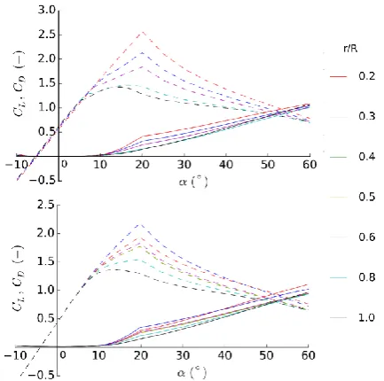
Coefficients against angle of attack at different points along the rotor radius for the Cases 1 and 3 are presented in Figure 7.

Figure 7 Blade local lift (dashed lines) and drag (solid lines) curves for Case 1 (top): NACA638(12-24), Re=3.0E+05 and Case 3 (bottom): NACA4415, Re=1.5E+05

IV.RESULTS A. BEM correction factors

As the BEM model requires correction factors to account for where physical effects are not captured, it is useful to determine the extent at which these are applied for assessments in their influence on the overall thrust and power predictions.

Figure 8 shows the axial induction factor and tip/hub loss correction factors calculated by the model for case 1b. From this, one can see that the model enters the ‘highly loaded regime’, based on the semi-empirical Buhl factor only at the tip and becomes more evident at higher TSRs. The tip/hub loss correction is significant, indicating large hydrodynamic losses particularly at low TSRs.

Figure 8 Case 1b normalised radial variation of axial induction factor and tip/hub loss correction factor at varying TSR

measurements with output from the BEM model in this study as well as other studies within the field of TST modelling.

Figure 9 shows that the present BEM model has excellent agreement with the 1/20th _{scale experimental data [8], and in in} line with a study using a research-led BEM model ‘SERG’ developed at Southampton University [11]. At the higher inflow velocity shown in Figure 10, there is again a strong correlation with measurements, however both models over predict power at high TSRs (>8) of up to 23%.

Figure 11 shows the BEM model performs very well with 1/60th _{scale parameters, showing again excellent agreement} with experiments [12]. The high levels of thrust seen at TSRs >4 is captured by the model, whereas a study using commercial software Tidal Bladed seems to show an under prediction of up to 10%.

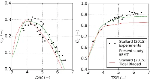
Figure 12 shows reasonable agreement with TSRs <3, however there are then over predictions in power and thrust. Results from CFD studies using a Hybrid RANS-BEM model, as well as a RANS fully blade resolved case [19] shows better agreement, however there is still an over prediction seen at TSRs >3. It was also noted that unlike previous cases, the numerical models also do not capture the optimal TSR where peak performance occurs. At peak TSR, BEM over predicts power by 28% and thrust by 20%.

Figure 9 Case 1a validation with 1/20th scale experiments at 1.3ms-1_{with12° pitch and SERG BEM model}

Figure 10 Case 1b validation with 1/20th scale experiments at 1.73ms-1 _{with 5° blade pitch and SERG BEM model}

Figure 11 Case 2 validation with 1/60th scale experiments a study using Tidal Bladed

Figure 12 Case 3 validation with 1/30th _{scale experiments and} CFD studies using RANS-BEM and RANS blade resolved cases Blade cyclic thrust loads

The average and cyclic thrusts experienced by each blade as the turbine passes through each rotation can be determined by the model, an example of which can be seen in Figure 13 for Case 1b. At higher velocities, the blade experiences higher thrusts, therefore the peak occurs at top dead centre. It can be seen that as the TSR increases, the average thrust increases, as to be expected from the CT curves. Additionally, it can also be seen that the variation of thrust forces also increases. At the optimal performance rotational velocity of 6 from Figure 10, the blade experiences fluctuations of around 20% around the rotor average.

C. Non-uniform blade loading

Additionally to the thrust levels for individual blades, the model also outputs the distribution of these thrusts down the blade length.

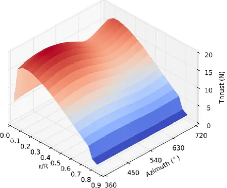
Figure 14 shows the thrust distribution with normalised rotor radius through one turbine rotation at the optimal performance rotational velocity. The peak again occurs at top dead centre, and it is seen that maximum values are seen close to the blade root.

Figure 14 Blade distribution of thrusts at optimal rotational velocity (TSR=6)

V. DISCUSSION

A. Validation

CP and CT curves from the model have excellent agreement with measurements for Cases 1 and 2, showing the methodology is well applied to these types of experiments. The strong correlations with other BEM models also show that the theory is well implemented in the code.

Over predictions in power, thrust and peak TSR are seen within Case 3 results at TSRs > 3, which are also seen (although less significantly) in the CFD studies. This error is thought to be a result of multiple causes:

1) Numerical errors in the generation of aero foil coefficients; 2) Measurement errors in the experiment;

3) Effects of high blockage correction and high widthwise velocity distributions seen across the channel;

4) Lack of free surface effects (CFD uses a volume of fluid free surface model).

Methods to combat these have been explored, including: CFD studies of 2D static aerofoils have been tested on NACA profiles, and show improved correlation to experimental data. This methodology may lower uncertainty in aerofoil coefficients, however are time intensive to generate. A free surface model developed by [9] could be applied to the model,

however difficulties have been identified when used in combination with the Buhl highly loaded correction factor.

To generate the CP and CT curves for each case, the present BEMT model took 3 minutes on a single quad core processor, equivalent to 0.05CPU-hours. In comparison, CFD studies of Case 3 reported a requirement of 12 CPU-hours for the RANS-BEM model, and 100 CPU-hours per turbine rotation of the RANS fully blade resolved model [20]. This indicates the significant computational savings of the present study, and hence its advantages in cases where processing time and ability to run on local machines outweighs the requirement for complex, high detailed simulations with wake characterisation. B. Blade loading

When a uniform inflow velocity is applied, blades experience a uniform thrust down its length. When non-uniform profiles are applied, such as in this case where a shear profile to account for boundary layer effects of the channel base, loading fluctuates as a function of azimuth. High fluctuations of almost 20% at the optimal rotational speed in Case 1b indicates the impact of just one component of the flow on loading conditions. Other inflow profiles could be applied to model actual flow regimes seen in the field, in order to gain cyclic loading information which could be used in a fatigue analysis.

Further assessment of the thrust forces shows that the blade is subjected to non-uniform loading along its length, which are not accounted for when considering average loads. Results are dependent on flow and operating conditions, however results from Case 1b at optimal TSR shows a peak occurs at a specific location along the blade. This shows the potential of using this tool as a methodology for attaining ‘hot spots’ where loads are concentrated, as well as generally more detailed loading information that can be used in Finite Element Analyses (FEA) to assess stress distributions. The resolution can be improved by splitting the blade into more elements.

It should be noted that this model considers steady, ‘frozen’ profiles, and is not optimised to consider dynamic inflows, which would be required to assess effects such as turbulence or waves. A time stepping function could be used to apply a series of different inflow profiles over time, however additional functions would need to be applied in order to consider dynamic effects such as inertia.

VI.CONCLUSIONS

iterative engineering assessments are made using low grade computational resources.

The model is then applied to assess the thrust and torque distributions along the blades, which can be used as more detailed inputs to FEA analyses as well as to determine localised ‘hotspots’ where stresses are concentrated. Additionally, fluctuating thrust forces as the turbine rotates through a non-uniform inflow profile are calculated, which can be used to determine cyclic loading conditions for a fatigue analysis. These indicate the potential of using this tool for improving the overall design process of turbine blades.

VII. FURTHER WORK

A methodology for attaining aerodynamic coefficients using CFD studies of static aerofoils in 2D flow are to be further developed in order to reduce uncertainty of the BEM inputs. This methodology will then be applied to ‘flat-plate’ aerofoil profiles, such as those seen in some full scale TSTs designs.

The model is currently under adaptation to perform assessments of the OpenHydro device, as high solidity, hubless and ducted turbine. Significant differences in design will be accounted for by using results from CFD studies and validations with a full scale deployment of a 2MW turbine at the Paimpol-Bréhat site in Jan 2016.

ACKNOWLEDGMENT

This research is carried out as part of the Industrial Doctoral Centre for Offshore Renewable Energy (IDCORE) programme, funded by the Energy Technology partnership and the RCUK Energy programme (Grant number EP/J500847/1), in collaboration with EDF R&D.

REFERENCES

[1] GL Garrad Hassan, “Tidal Bladed Theory Manual,” 2012.

[2] I. Masters, J. Chapman, M. Willis, and J. Orme, “A robust blade element theory model for tidal stream turbines including tip and hub loss corrections,” J. Mar. Eng. Technol., vol. 10, no. 1, pp. 25–35, 2011.

[3] T. Burton, Wind Energy Handbook. 2011.

[4] R. E. Wilson and P. B. S. Lissaman, “Applied aerodynamics of wind power machines,” 1974.

[5] M. L. Buhl, “A New Empirical Relationship between Thrust Coefficient and Induction Factor for the Turbulent Windmill State A New Empirical Relationship between Thrust Coefficient and Induction Factor for the Turbulent Windmill State,” 2005.

[6] J. C. Chapman, I. Masters, M. Togneri, and J. a C. Orme, “The Buhl correction factor applied to high induction conditions for tidal stream turbines,” Renew. Energy, vol. 60, pp. 472–480, 2013.

[7] C. Garrett and P. Cummins, “The efficiency of a turbine in a tidal channel,” vol. 588, pp. 243–251, 2007.

[8] A. S. Bahaj, A. F. Molland, J. R. Chaplin, and W. M. J. Batten, “Power and thrust measurements of marine current turbines under various hydrodynamic flow conditions in a cavitation tunnel and a towing tank,” Renew. Energy, vol. 32, no. 3, pp. 407–426, 2007.

[9] J. I. Whelan and J. M. Graham, “A free surface and blockage ratio correction for tidal turbines,” Fluid Mech., vol. 624, pp. 281–291,

2009.

[10] C. Buvat and V. Martin, “ETI PerAWaT Report: WG4 WP1 D1 Identification of test requirements and physical model design,” 2010.

[11] A. S. Bahaj, W. M. J. Batten, and G. McCann, “Experimental verifications of numerical predictions for the hydrodynamic performance of horizontal axis marine current turbines,” Renew. Energy, vol. 32, no. 15, pp. 2479–2490, 2007.

[12] T. Stallard, T. Feng, and P. K. Stansby, “Experimental study of the mean wake of a tidal stream rotor in a shallow turbulent flow,” J. Fluids Struct., vol. 54, pp. 235–246, 2015.

[13] C. Buvat, “ETI PerAWaT Report: WG4 WP1 D4 Performance of tank tests with physical scale model of horizontal axis turbine device installed,” 2012.

[14] J. I. Whelan and T. J. Stallard, “Arguments for modifying the geometry of a scale model rotor,” 9th Eur. Wave Tidal Energy Conf. Southhampt., 2011.

[15] I. H. Abbott, A. E. Von Doenhoff, and L. S. Stivers, “Summary of Airfoil Data, Report no. 824,” Langley, 1945.

[16] S. Miley, “A catalogue of low reynolds number airfoil data,” 1982.

[17] S.-P. Brenton, F. N. Coton, and M. Geir, “A Study on Different Stall Delay Models Using a Prescribed Wake Vortex Scheme and NREL Phase VI Experiment,” in EWTEC 2007, 2007.

[18] S. A. Ning, “AirfoilPrep documentation,” no. June, 2013.

[19] S. C. Mcintosh, C. F. Fleming, and R. H. J. Willden, “Embedded RANS-BEM Tidal Turbine Design,” Cell.