The Minimum Cost Design of Transparent Optical
Networks Combining Grooming, Routing,
and Wavelength Assignment
Agostinho Agra, Amaro de Sousa, and Mahdi Doostmohammadi
Abstract— As client demands grow, optical network operators are required to introduce lightpaths of higher line rates in order to groom more demand into their network capacity. For a given fiber network and a given set of client demands, the minimum cost network design is the task of assigning routing paths and wavelengths for a minimum cost set of lightpaths able to groom all client demands. The variant of the optical network design problem addressed in this paper considers a transparent optical network, single hop grooming, client demands of a single interface type, and lightpaths of two line rates. We discuss two slightly different mixed integer linear programming models that define the network design problem combining grooming, routing, and wavelength assignment. Then, we propose a parameters increase rule and three types of additional constraints that, when applied to the previous models, make their linear relaxation solutions closer to the integer solutions. Finally, we use the resulting models to derive a hybrid heuristic method, which combines a relax-and-fix approach with an integer linear programming-based local search approach. We present the computational results showing that the proposed heuristic method is able to find solutions with cost values very close to the optimal ones for a real nation-wide network and considering a realistic fiber link capacity of 80 wavelengths. Moreover, when compared with other approaches used in the problem variants close to the one addressed here, our heuristic is shown to compute solutions, on average, with better cost values and/or in shorter runtimes.
Index Terms— Optical transport networks, grooming, routing and wavelength assignment, mixed integer linear programming, valid inequalities, hybrid heuristics.
I. INTRODUCTION
C
ONSIDER a transparent optical network composed by a set of optical switching nodes and a set of fibers, each one connecting a pair of nodes. In modern fixed gridManuscript received December 30, 2014; revised August 14, 2015 and February 3, 2016; accepted March 8, 2016; approved by IEEE/ACM TRANS
-ACTIONS ONNETWORKINGEditor D. Medhi. The work of A. Agra and M. Doostmohammadi was supported by the Fundação para a Ciência e a Tecnologia under Grant UID/MAT/04106/2013 and the program COMPETE: FCOMP-01-0124-FEDER-041898 under Grant EXPL/MATNAN/1761/2013. The work of A. de Sousa was supported under Grant UID/EEA/50008/2013 and the Project “Optimizing Next-generation Elastic Core Network Infrastruc-ture” under Grant PTDC/EEITEL/3303/2012.
A. Agra is with the Centro de Investigação e Desenvolvimento em Matemática e Aplicações (CIDMA), Departamento de Matemática, Universidade de Aveiro, Aveiro 3810-193, Portugal (e-mail: [email protected]).
A. de Sousa is with the Instituto de Telecomunicações/DETI, Universidade de Aveiro, 3810-193 Aveiro, Portugal (e-mail: [email protected]).
M. Doostmohammadi is with the Centro de Investigação e Desenvolvimento em Matemática e Aplicações (CIDMA), Departamento de Matemática, Uni-versidade de Aveiro, Aveiro 3810-193, Portugal, and also with the Instituto de Engenharia Mecânica (IDMEC), Instituto Superior Técnico, University of Lisbon, Lisbon 1649-004, Portugal (e-mail: [email protected]).
Digital Object Identifier 10.1109/TNET.2016.2544760
networks, the spectrum of each fiber is organized in a set T of|T|different wavelengths of 50 GHz spectrum width where, typically, |T|= 80. Data is transmitted from its source node to its destination node by lightpaths which are optical paths crossing a set of fibers and using one wavelength on each fiber. In a transparent optical network, a lightpath must be assigned with the same wavelength on all fibers of its path. For a given set of lightpaths to be established on a given fiber network, the classical Routing and Wavelength Assignment (RWA) problem consists in assigning a routing path and a wavelength for each lightpath, aiming to optimize a given target objective.
Since data is in the electrical domain and lightpaths are in the optical domain, a pair of electrical-optical converters, named transponders, is placed on the end nodes of each lightpath. Moreover, the optical signal propagation is affected by different factors like attenuation, dispersion, crosstalk and other non-linear factors, commonly named physical impair-ments, which limit the maximum length the signal can be propagated from transmitter to receiver. To work properly, a lightpath has an associated maximum length, commonly named transparent reach. If a lightpath is required on a path whose length is higher than its transparent reach, regenerators must be placed at one or more intermediated nodes of the lightpath (a regenerator is a back-to-back pair of transponders that recovers the optical signal into the electrical domain and resends it back to the optical domain). Nevertheless, the use of regenerators is expensive and puts an additional burden on the network management and, therefore, they are avoided when possible (when regenerators are used, the network is referred to as a translucent network).
Modern optical networks allow the client demands to be groomed on lightpaths, i.e., multiple client demands grouped to be transmitted over a single lightpath. This has two benefits: it reduces the required number of lightpaths and it enlarges the total transmission capacity of the network. In this case, the transponders at the end nodes of a lightpath have one multiplexer coupled to each of them (a transponder coupled with a multiplexer is named a muxponder). The Optical Trans-port Network (OTN) ITU-T G.709 recommendation defines the grooming alternatives and resulting line rates for different types of client demand interfaces. In this recommendation, grooming is implemented in an electrical layer, named Optical Transport Unit (OTU), and there are different OTU types to support different client interface types. For example, for client interfaces of10Gbps Ethernet type: (i) one such interface can be transmitted in a lightpath of type OTU-2 with a line rate of
approximately 10 Gbps (in this case, there is no grooming), (ii) four such interfaces can be groomed into a lightpath of type OTU-3 with a line rate of approximately 40 Gbps or (iii) ten such interfaces can be groomed into a lightpath of type OTU-4 with a line rate of approximately 100 Gbps.
Each lightpath alternative has its own associated cost and transparent reach and, in practice, lightpaths of higher line rates can groom more client demands at the cost of being more expensive and having shorter transparent reach. The Grooming, Routing and Wavelength Assignment (GRWA) network design problem is the combination of the grooming problem with the classical RWA problem and consists in assigning routing paths and wavelengths for a minimum cost set of lightpaths able to groom all client demands.
In general, we can distinguish two grooming types: single hop and multi hop grooming. In single hop grooming, light-paths groom only client demands between their end nodes. In multi hop grooming, a client demand can be groomed with some other demands into a lightpath from its source node to an intermediate node and groomed again with other demands from the intermediate node to its destination node (this is the two hop grooming case but the idea can be generalized to multiple hops). Although some gains can be achieved with lightly loaded networks, these gains become marginal for reasonably loaded networks (most lightpaths become fully occupied with direct demands) and, since it makes network management more complex, network operators usually resort to single hop grooming only.
We address the GRWA network design problem in the context of a network operator with a highly loaded network based on lightpaths of a given OTU type who aims to upgrade it by introducing lightpaths of the next higher line rate OTU type. Such lightpaths enable it to support more client demands preventing the network to become fully occupied. So, the operator aims to compute the lowest cost set of lightpaths able to groom all its client demands allowing lightpaths of the two OTU types to coexist on its network. The GRWA network design problem addressed in this paper considers a transparent optical network, single hop grooming, client demands of a single interface type and lightpaths of two line rates.
Since GRWA (and, also, RWA) is NP-hard, most previous works addressing these problems either propose pure heuris-tic approaches or decompose the problem into subproblems (grooming problem+routing problem+wavelength assign-ment problem) and solve them sequentially. Although the decomposition approach can be exact when the network is lightly loaded (in this case, the grooming optimal solution can be computed separately since there is always a RWA solution for any grooming configuration), this is not our case of interest. Some works (reviewed in the next section) have proposed integer linear programming formulations for the classical RWA problem and, more recently, for the harder GRWA problem but the reported results have shown so far that they can deal with problem instances significantly smaller than the real cases. Nevertheless, using advanced integer linear program-ming modeling techniques, together with the huge increase of computer CPU processing capacity (multiple core CPUs and multi-thread solver packages) and RAM memory capacity, we
can now aim to use integer linear programming to deal with real sized problem instances.
In this paper, we first discuss two slightly different mixed integer linear programming models that define the GRWA net-work design problem. Then, we improve them with strength-ening techniques (one based on increasing some problem parameters and the others based on three types of additional constraints) that, when applied to the previous models, make their linear relaxation solutions closer to the integer solutions. Finally, we use the resulting models to derive a hybrid heuris-tic method which combines a relax-and-fix approach with an integer linear programming based local search approach. We present computational results showing that this heuristic is able to find solutions with a cost value very close to the opti-mal one. Moreover, when compared with previous approaches (used in problem variants close to the one addressed here), the proposed heuristic is shown to compute solutions, on average, with better cost values and/or in shorter runtimes.
This paper is organized as follows. Section II presents the previously published related work. Section III discusses the two formulations defining our GRWA problem variant, together with a method to compute valid lower bounds and a decomposition that is used by other works. Section IV describes the different techniques used to strengthen the pre-vious formulations. Section V presents the hybrid heuristic. The computational results are described and discussed in Section VI. Finally, Section VII presents the main conclusions.
II. RELATEDWORK
The classical RWA problem is known to be NP-hard [1]. It has been extensively studied in the literature although only some of the works have dealt with efficient integer linear programming formulations for it. In [2], Integer Linear Programming (ILP) models are proposed for the RWA problem assuming that wavelength conversion is available on network nodes (a problem variant that makes the problem tractability much easier) and the aim is to minimize the average number of demand routing hops. In [3], different ILP models for the RWA network design problem are compared (a flow based formulation and a source based formulation) addressing both cases with or without wavelength conversion. Nevertheless, the computational results reported in both works ([2], [3]) show that only problem instances with a fiber capacity up to10wavelengths can be solved to optimality. Finally, in [4], different path-based formulations are compared to solve the RWA problem aiming to maximize the total number of estab-lished lightpaths. They show that branch-and-price methods can solve the problem more efficiently than using compact models (i.e., models with a polynomial number of variables) and the computational results show that near optimal solutions can be obtained for relevant sized networks with fiber capacity of up to 34 wavelengths. A similar approach was also proposed in [5] with more modest computational results, also due to the computational resources available by then.
longer transparent reach values for each lightpath if wave-lengths are assigned on each fiber minimizing the interference between them. In [6], this problem is addressed showing that efficient ILP models to define such problem are quite hard. In [7], the authors propose ILP models, for small and medium sized transparent networks and, since the models are hard to solve larger networks, a three-phase heuristic is proposed. In [8], the authors propose a heuristic where the RWA problem is decomposed into its routing and wavelength assignment subproblems which are solved separately. Nevertheless, the transparent reach gains, while considering the impairment aware variant, are only possible with lightly loaded networks where only a few wavelengths are required on each fiber. When total demand is significant, most of the wavelengths have to be used in all fibers and the transparent reach of each lightpath becomes a conservative value independent of the wavelengths assigned to the other lightpaths.
The GRWA problem, which is much harder than the clas-sical RWA problem, has been also addressed in recent works. In [9], an additional constraint is considered on the maximum number of transceivers on each node and the objective is the throughput maximization (it is assumed that the network cannot accommodate the total required demand). The authors propose a path-based formulation and, since computational results show that only small network sizes can be dealt with, they propose a heuristic based on column generation techniques. In [10], the GRWA network design problem is addressed considering the minimization of the number of lightpaths. They solve to optimality a test instance with 6 nodes with a fiber capacity of up to 30 wavelengths (still significantly lower than the capacity of current optical net-works). For bigger instances, they propose the decomposition of the problem in two subproblems (Grooming problem + RWA problem) that are solved sequentially. For heavily loaded networks, though, this decomposition might fail since the solution of the grooming problem might be unfeasible to the RWA problem. Some works ([11], [12]) use path based formulations and branch-and-price as a solution technique but also do not consider the wavelength continuity constraints. Other works use a reduced set of candidate paths ([11], [13]) to make the methods scalable for larger problem instances. This approach will be compared with our approach in Section VI. All these previous works dealing with the GRWA prob-lem consider that all lightpaths are of the same line rate. In [14], though, the authors deal with the mixed line rates case. They propose the decomposition of the problem in the Grooming and Routing (GR) subproblem and the Wavelength Assignment (WA) subproblem that are solved sequentially. They start by solving the two subproblems considering a fiber capacity of T wavelengths. If the solution of GR makes the WA unfeasible, they decrementT and repeat the process. This approach will be compared with our approach in Section VI.
As a final remark, note that network design problems fall in the category of static (G)RWA problems. On the other hand, dynamic problems consider that demand requests arrive randomly, one at a time, and last in the network a finite random time. In this case, the aim is to optimize some performance metric like blocking probability (see [15]–[17]).
III. MIXEDINTEGERLINEARPROGRAMMINGMODELS
Consider a fiber network defined by the graphG= (N, E) such that the spectrum of each fiber e ∈ E is organized in a set T of |T| wavelengths. Consider a set of demand pairs D such that each demand pair d ∈ D is a node pair that has at least one client demand between them. So, a demand pair d∈ D is defined by a pair of end nodes in G and an integer demand valuevd with the aggregated number
of client demand interfaces that must be supported between its end nodes. To support the demands of each d ∈ D, consider two types of lightpaths (type 1 and 2) that can be set on the fiber network, defined by their capacitiesδ1 andδ2 (in number of client demand interfaces), respectively, such that δ1 < δ2. Since we consider single hop grooming, the end nodes of each lightpath are the end nodes of the demand pair supported by it (note that different lightpaths supporting the client demand interfaces between the same end nodes can be routed differently).
Each lightpath can be set in the underlying fiber network through a routing path whose length cannot be higher than its transparent reach and lightpaths with higher line rates have lower transparent reach values. So, the transparent reachl1of a lightpath of type1is higher than the transparent reachl2of a lightpath of type2. ConsiderPd as the set of all routing paths
for lightpaths of type 1 between the end nodes of demand paird∈D whose total length is not higher thanl1. For each routing path p ∈ Pd, the binary parameter αp is one if the
total length ofpis also not higher thanl2. A lightpath of type i ∈ {1,2} routed in path p ∈Pd between the end nodes of
d ∈ D has an associated cost of cpi, such that cp1 < cp2.
Additionally, consider the set P = d∈DPd of all routing
paths and, from this set, the subsetsPeas the sets of all routing
paths that include fibere∈E.
Consider the following variables. Variable xpti indicates
the amount of demand routed through path p∈ P with the assigned wavelength t ∈ T and using a lightpath of type i∈ {1,2}. Binary variableyptitakes the value1if pathp∈P
is in the solution with the assigned wavelength t ∈ T as a lightpath of typei∈ {1,2} (it takes value 0, otherwise). The GRWA network design problem can be formulated as:
min
p∈P
t∈T
2
i=1
cpiypti, (III.1)
s.t.
p∈Pd
t∈T
2
i=1
xpti=vd, d∈D, (III.2)
xpt1≤δ1ypt1, p∈P, t∈T, (III.3)
xpt2≤αpδ2ypt2, p∈P, t∈T, (III.4)
p∈Pe
2
i=1
ypti≤1, e∈E, t∈T, (III.5)
xpti≥0, p∈P, t∈T, i∈ {1,2}, (III.6)
ypti∈ {0,1}, p∈P, t∈T, i∈ {1,2}. (III.7)
lightpaths have enough capacity to groom their supported client demands. Constraints (III.5) ensure that, on each fibere, each wavelength t is assigned to at most one lightpath. Constraints (III.6) and (III.7) are the variable domain constraints.
Alternatively, consider variables xpt representing the
demand that is routed through path p ∈ P in the solution with the assigned wavelength t∈T, i.e.:
xpt=
2
i=1
xpti, (III.8)
With these new variables, the GRWA network design prob-lem can be formulated as:
min
p∈P
t∈T
2
i=1
cpiypti, (III.9)
s.t.
p∈Pd
t∈T
xpt=vd, d∈D, (III.10)
xpt≤δ1ypt1+αpδ2ypt2, p∈P, t∈T, (III.11)
p∈Pe
2
i=1
ypti≤1, e∈E, t∈T, (III.12)
xpt≥0, p∈P, t∈T, (III.13)
ypti∈ {0,1}, p∈P, t∈T, i∈ {1,2}. (III.14)
Henceforward we consider the following two mixed integer linear programming models: Model1defined by (III.1)–(III.7) and Model2defined by (III.9)–(III.14). In terms of complex-ity, the number of constraints is O(max{|D|,|P| · |T|})and the number of variables is O(|P| · |T|)in both models. In the general case, |P| increases exponentially with the graph size but in our case the transparent reach of the lightpaths keeps this number within reasonable values for relevant sized graphs. Next, we provide two important remarks.
Remark 1: Constraints (III.11) are obtained by summing up constraints (III.3) and (III.4), and applying (III.8). Thus, relating the two models by summing up variables xpti,
i ∈ {1,2}, and adding constraints (III.8) to the second
model, one can easily check that the aggregated Model 2 is weaker than Model 1, in the sense that the projection of its linear relaxation set contains the linear relaxation of constraints (III.2)–(III.7). However, since the xvariables do not appear in the objective function one can also check that the linear relaxation of both models provides the same lower bound.
Remark 2: One can check that the matrix of coefficients of
xvariables is totally unimodular in both models, that is, each square submatrix of the matrix of coefficients has determinant
0,−1,or+1.Therefore, for each binary set of values for the
y variables the linear relaxation of the resulting feasible set will always provide integer values for xvariables, see [18] for details. Hence, we can drop the integrality requirements onxvariables in both models, as defined in constraints (III.6) and (III.13).
Based on these two remarks, we might expect that Model2 is better than Model 1 since it has slightly less number of constraints and half of the real variables although the number
of integer variables remains the same. Nevertheless, with the improvements described in the next section, the computational results show that the resulting methods based on Model 1 obtain solutions with lower cost values.
Note that, when removing constraints (III.5) on Model1and maintaining the integrality of the ypti variables, the problem
becomes easy to solve since it can be separated in a set of subproblems, one for each d ∈ D. This is an easy way to determine valid lower bounds that will be used in the computational results. Assuming that cpi =ci, for all p∈P
(since in a transparent network regenerators are not used), the subproblem associated with demand pair d ∈ D becomes a 2-dimensional knapsack problem defined as:
min{c1Y1+c2Y2:δ1Y1+δ2Y2≥vd, Y1, Y2∈Z+},
where Y1 =
p∈Pd
t∈Typt1
and Y2 =
p∈Pd
t∈Tαpypt2.
This
subproblem can be efficiently solved by an algorithm based on the Euclidean algorithm (see [19] for details).
The overall problem can be decomposed in different ways and many works use different decompositions to derive solu-tion techniques. The one used in [14] decomposes the problem in the Grooming and Routing (GR) problem and the Wave-length Assignment (WA) problem. Since the method of [14] will be used in the computational results, we formally define this decomposition. The GR problem is modeled as:
min
p∈P
2
i=1
cpiYpi, (III.15)
s.t.
p∈Pd
2
i=1
Xpi=vd, d∈D, (III.16)
Xp1≤δ1Yp1, p∈P, (III.17) Xp2≤αpδ2Yp2, p∈P, (III.18)
p∈Pe
2
i=1
Ypi ≤K, e∈E, (III.19)
Xpi ≥0, p∈P, i∈ {1,2}, (III.20)
Ypi∈ {0,1}, p∈P, i∈ {1,2}, (III.21)
where K = |T|, Xpi =
K
t=1xpti and Ypi =
K
t=1ypti.
The new variables are aggregated versions of the original ones and GR assigns a routing path to each lightpath ensuring that the fiber capacities are not exceeded. The WA subproblem determines a wavelength assignment to the lightpaths of the GR solution. In order to define an objective function to WA, we use the minimization of the number of used wavelengths. Let wt be a binary variable indicating whether wavelengtht
is used or not. Given a solution (X∗, Y∗) of GR, the WA problem is modeled as:
min
t∈T
wt, (III.22)
s.t.
t∈T
ypti=Ypi∗, d∈D, p∈Pd, i∈ {1,2}, (III.23)
ypti≤wt, p∈P, t∈T, i∈ {1,2}, (III.24)
wt≤wt−1, t∈T, t >1, (III.25)
wt∈ {0,1}, t∈T, (III.26)
where constraints (III.23) guarantee that a wavelength t∈T is assigned to each lightpath defined in Y∗.
IV. IMPROVEMENTS
It is well-known that the derivation of strong formulations is of key importance to solve mixed integer linear program-ming problems using Branch and Cut (B&C) algorithms [18]. The linear programming (LP) relaxation of a problem is the problem considering the original formulation with the integer variables replaced by real variables (i.e., obtained by replacing constraints (III.7) or (III.14) by 0 ≤ ypti ≤ 1).
The performance of B&C depends on how close the fractional solutions of the LP relaxation are from the integer solutions of the original problem. Linear programming techniques able to cut off fractional solutions from the LP relaxation feasible set while maintaining all integer solutions of the original problem make the formulations stronger in the sense that B&C is able to find either an optimal solution in shorter runtime or a better solution for the same runtime limit. In this section, we describe two types of techniques to derive stronger formulations while keeping the total number of constraints of the model under control. The first type is the increase of the demand values. The second type is related with the addition of different constraints. These constraints are based on valid inequalities derived for simple mixed integer sets arising from relaxations of the original feasible set. We describe these improvements in detail in the following subsections.
A. Demand Values Increase
Since the cost of a solution depends only on the lightpaths and is not influenced on how occupied each lightpath is, we can increase the demand values provided that the required set of lightpaths remains unchanged. By increasing the demand valuesvd, d∈D,we force the values of somexvariables to
increase, which forces the values ofyvariables also to increase in the LP relaxation (due to constraints (III.3) and (III.4) in Model 1 or (III.11) in Model 2). Note that the demand values increasing rule is parameter dependent. For δ1 = 4 and δ2 = 10, as considered in our problem instances, the possible values for the installed lightpaths capacity are the positive values given by all nonnegative integer linear combinations of 4 and10, which are4,8,10,12,14,16, . . .. Hence, the demand values increasing rule is: for each d∈D, (i) we set vd = 4 if vd < 4, (ii) we set vd = 8 if
4 < vd < 8 and (iii) we set vd = vd + 1 if vd > 8
and odd.
B. Valid Inequalities
[image:5.612.345.521.53.163.2]One possible approach to derive valid inequalities for a mixed integer linear problem is, first, to identify sim-ple mixed integer sets arising as relaxations of the origi-nal feasible set. Consider the set of feasible solutions of Model 1 defined by X. In this section, we discuss three different relaxation sets of X for which valid inequalities are known. Using such inequalities, we derive valid inequalities forX.
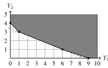
Fig. 1. Facet-defining inequalities for conv({(Y1, Y2) ∈ Z2 | 4Y1 +
10Y2≥34}, Y1, Y2≥0).
1) Integer Knapsack Relaxation: A first relaxation is
obtained for each d ∈ D from inequalities (III.2), (III.3) and (III.4) as follows:
p∈Pd
t∈T
(δ1ypt1+δ2αpypt2)≥
p∈Pd
t∈T
(xpt1+αpxpt2) =vd.
Setting Y1 =
p∈Pd
t∈T
ypt1 and Y2 =
p∈Pd
t∈T
αpypt2, the previous inequality can be written as
δ1Y1+δ2Y2≥vd. (IV.1)
Thus, the following two integer variables knapsack set is obtained as a relaxation ofX.
XIK=
(Y1, Y2)∈Z2 | δ1Y1+δ2Y2≥vd, Y1, Y2≥0
.
The strongest valid inequalities forXIK are the facet-defining
inequalities which, for such sets, can be derived in polynomial time [19] and whose coefficients are obtained, in general, using the euclidian algorithm. The number of facet-defining inequal-ities is polynomial. For the particular case of coefficients considered in the computational results (δ1= 4andδ2= 10), we have at most four non-trivial facet-defining inequalities for eachd∈D(Y1≥0andY2≥0 are called trivial), which are of the following forms:2Y1+ 5Y2≥
vd
2
+ 1,Y1+ 3Y2 ≥
vd
4
+ 1, Y1+ 2Y2 ≥
vd
5
+ 1 and Y1+Y2 ≥
vd
10
+ 1 leading to the following valid inequalities forX:
2
p∈Pd
t∈T
ypt1+ 5
p∈Pd
t∈T
αpypt2 ≥
v
d
2
+ 1,
p∈Pd
t∈T
ypt1+ 3
p∈Pd
t∈T
αpypt2 ≥
v
d
4
+ 1,
p∈Pd
t∈T
ypt1+ 2
p∈Pd
t∈T
αpypt2 ≥
v
d
5
+ 1,
p∈Pd
t∈T
ypt1+
p∈Pd
t∈T
αpypt2 ≥
v
d
10
+ 1.
Example 3: Let vd = 34, for some d ∈ D. So XIK =
{(Y1, Y2)∈Z2 |4Y1+ 10Y2≥34, Y1, Y2≥0}. The segment
line4Y1+10Y2= 34is drawn by dashed line in Fig. 1. As it is
shown in Fig. 1, the convex hull ofXIK has three non-trivial
facet-defining inequalities:2Y1+5Y2≥17,Y1+3Y2≥9, and Y1+Y2 ≥4. Note that, for vd = 34, one of the inequalities
These inequalities can be added a priori to the models or added dynamically, that is, an inequality is added when the fractional solution violates that inequality. These inequalities can also be extended to the case where more than two types of lightpaths are considered, as described in [20].
2) Clique Inequalities: A common relaxation, when
incom-patibility between binary variables is considered (i.e., variables that cannot simultaneously assume value 1 in the solution) is the vertex packing set. These incompatibilities are often called conflicts and are represented in a conflict graph where nodes represent variables and edges represent incompatibil-ity between two binary variables. Given a conflict graph G = (N,E), the vertex packing set [21] is defined as XV P =
z ∈ {0,1}n | z
u +zv ≤ 1,(u, v) ∈ E
, where zu is a binary variable indicating whether nodeuis selected
or not andn=|N |.
Here, each node u of the conflict graph in N is a triple (p, t, i) that corresponds to a variable ypti and there is an
edge in E between two nodes (p, t, i) and (p, t, i), if the corresponding variables cannot be set simultaneously to one, that is, ypti+ypti ≤ 1. Constraints (III.5) impose
incom-patibility between all pairs of variables representing lightpaths that use the same wavelength on the same fiber. A complete description of the convex hull ofXV P is not known and since
optimizing a linear function overXV P is NP-hard, there is no
much hope in finding such a description. Nevertheless, families of valid inequalities are known [18] and one of the most well-known families is the set of clique inequalities. A clique in a graph is a subset of nodes such that for each pair of nodes in the subset there exists an edge connecting them. In the present case, a clique is a set of variables that are pairwise incompatible. Then, the following result stands:
Proposition 4: IfC⊂ N is a clique in the conflict graphG,
then the inequality (called clique inequality)
(pti)∈C
ypti≤1, (IV.2)
is valid forX.
A maximal clique is a clique that cannot be extended by including one more adjacent node, meaning it is not a subset of a larger clique. It is well-known that only clique inequalities associated with maximal cliques need to be considered [21]. As the number of clique inequalities can increase exponen-tially with the number of variables, this family of inequalities is, in general, added dynamically.
Our preliminary experiences showed that there are too many clique inequalities resulting in too large models (some of these clique inequalities can also be identified and added auto-matically by the solver). Therefore, we focused on deriving clique inequalities that use the knowledge of the structure of the GRWA network design problem. A family of clique inequalities that was shown to be effective in cutting off fractional solutions with a small number of inequalities is as follows. We define a Y-structure of a network as a subgraph which contains four nodes with the structure shown in Fig. 2 where node B is the central node. Considering the conflicts
Fig. 2. Y-structure subgraph.
arising from Y-structures, fort∈T, the clique inequality
p∈PB
2
i=1
ypti≤1,
is valid for X where
PB=
p∈P |ppasses through central nodeB
.
In order to identify these clique inequalities, we identify each Y-structure on the fiber network defined by the graph G = (N, E) (note that each node on N with a degree of 3 is the central node of a Y-structure) and add the value of all ypti variables representing paths that include two edges of the
Y-structure. If the total value is greater than one, then the corresponding clique inequality (IV.2) is added.
3) Mixed Integer Rounding (MIR) Inequalities: MIR is a
technique to derive strong valid inequalities for mixed integer sets. The well-known MIR inequalities [18] can be stated as follows.
Proposition 5: Consider the simple mixed integer set
XSMI ={(S, Y)∈R+×Z|S+aY ≥b}where a, b∈R+
are arbitrary constants. The inequality (called MIR inequality)
S≥r b/a −Y, (IV.3)
is valid forXSMI, wherer=b−(b/a −1)a.
Next, we apply this proposition to derive valid inequalities for X. In order to do that, we define mixed integer sets of the form of XSMI that result from the relaxation of X. For
each lightpath type i ∈ {1,2}, each demand pair d ∈ D and considering a subset of paths P ⊂ Pd and a subset
of wavelengths T ⊂ T, we use constraints (III.2), (III.3) and (III.4) to show that:
p∈Pd
t∈T
j∈{1,2}|j=i
αpjxptj+
p∈Pd\P
t∈T\T
αpixpti
+
p∈P
t∈T
αpiδiypti≥
p∈Pd
t∈T
2
j=1
αpjxptj=vd.
whereαp1 = 1 and αp2 =αp. To obtain this inequality, we
start from constraint (III.2) and replace variables xpti (with
p∈P andt∈T) with the termδiypti(ifi= 1) coming from
constraints (III.3) or the termαpδiypti(ifi= 2) coming from
constraints (III.4). In this way, for a given typeiand demand paird, the inequality (IV.3) holds by setting
S =
p∈Pd
t∈T
j∈{1,2}|j=i
αpjxptj+
p∈Pd\P
t∈T\T
αpixpti,
Y =
p∈P
t∈T
Fig. 3. MIR inequality forXM ={(S, Y)∈R+×Z|S+ 4Y ≥14}.
Algorithm 1 Relax and Fix Algorithm
1: Solve the LP relaxation of Model1with increased demand values
2: repeat
3: Identify and add violated inequalities
4: Solve the LP relaxation of the resulting model
5: until no new violated inequalities are found
6: Set (x, y)to the fractional solution
7: Set variablesypti to one if ypti = 1 and run solver for at
mostT ime1 seconds
8: Set variables ypt2 to one ifypt 2= 1 and run solver for at
mostT ime1 seconds
9: Set (x, y) to the best solution found
Example 6: Let a = δ1 = 4 and vd = 14. In Fig. 3, the
facet of the convex hull ofXSMIdefined by the MIR inequality
S+ 2Y ≥ 8 ⇔ S ≥2(4−Y) is the line segment between points(0,4) and(2,3).
In order to identify the MIR inequalities, we have to decide whether each pair (p, t) belongs to (P , T)or not. We select one MIR inequality for eachi∈ {1,2}and eachd∈Din the following way: for a given relaxation solution, we compare the value of xpti with r·ypti and put (p, t) in (P , T) if
xpti> r·ypti.
V. HYBRIDHEURISTICPROCEDURE
As we are dealing with an NP-hard problem, one can hardly expect to solve all problem instances to optimality within reasonable runtime limits. Hence, in this section, we propose a heuristic procedure combining two algorithms: a Relax and Fix Algorithm that aims at finding an initial feasible solution and a Local Search Algorithm that aims at improving the feasible solution provided by the first algorithm.
In the Relax and Fix Algorithm (see Algorithm 1), we start by determining a fractional solution (x, y) (steps1 to 6) in the following way: we solve the LP relaxation of Model1with the demand values increasing rule as defined in the previous section (Step 1) and, then, we add the valid inequalities that are violated and solve again the LP relaxation until no new violated inequalities are found (steps2 to 5). The addition of the valid inequalities follows the order: Knapsack, MIR, and Clique inequalities (the computational tests have shown that this order leads to the smallest number of added inequalities, keeping the size of the models as small as possible).
Then, some of the y binary variables with value 1 in the fractional solution (x, y) are fixed to 1 and the resulting
Algorithm 2 Local Search Algorithm
1: repeat
2: Fix the variablesypt1 to one ifypt 1= 1andypt1= 1
3: Add inequality (V.1)
4: Run solver for at mostT ime2 seconds
5: If a better solution is found then update(x, y)
6: until No improvement is obtained
restricted integer model is solved with a runtime limit of T ime1. We have considered two fixing strategies: (i) fix to1 all ypti variables i.e., for both types of lightpaths i ∈ {1,2}
that have value1 (step 7) and (ii) fix to 1 the ypt2 variables
(i.e., only for lightpaths of type2) that have value1(step 8). In the first case, we have a more restrictive integer model that is solved in shorter runtime but has a lower probability of being feasible. In the second case, we have a less restrictive integer model that is solved in longer runtime but has a higher probability of being feasible. If both approaches provide a feasible solution, the best one is chosen (step 9).
The Local Search Algorithm (see Algorithm 2) takes as input the best solution, denoted by (x, y), obtained by the previous algorithm, and searches for better solutions in a neighborhood of this solution. This neighborhood is charac-terized by those solutions such that the number of lightpaths assigned to a path and/or to a wavelength that differs from the one in y is at most Δ. From a modeling point of view, this corresponds to adding (in step 3) a constraint ensuring that at mostΔ variables ypti can have a different value from the
value they have in solution(x, y), which is given byypti:
p∈P,t∈T,i∈{0,1}|ypti=0 ypti
+
p∈P,t∈T,i∈{0,1}|ypti=1
(1−ypti)≤Δ. (V.1)
The first term counts the number of variablesypti that have a
value0in(x, y)and flip their value to1while the second term counts the number of variablesyptithat have a value1in(x, y)
and flip their value to 0. Then, we solve the resulting model for at most T ime2 seconds (step 4), update the best feasible solution if a better solution is found (step 5) and repeat the process until no improvement is obtained (step 6). In order to speed up the algorithm, we fix to 1 all variables that have value1 in both the fractional and the best solution (step 2).
Note that Δ, T ime1 and T ime2 are parameters of the heuristic procedure. For the problem instances considered in the computational results, and after some preliminary com-putational tests, we have observed that the best trade-off between the quality of the final solution and the runtime to find it, on average, was obtained with the parametersΔ = 5, T ime1= 1500seconds andT ime2= 600seconds.
αp= 1 we set xpt1= 0andypt1= 0 in Model 1). We solve
this model (which is much easier). If the problem is feasible, the feasible solution is given as input to the Local Search Algorithm. Otherwise, we show that the problem is infeasible. As a final remark, note that two alternative approaches for the Relax and Fix Algorithm used in other works could be as follows. After computing the fractional solution (x, y), the initial solution (x, y) is determined by (i) applying rounding techniques or (ii) solving the integer problem restricted to the non-null variables of (x, y). Our computational tests have shown that the proposed Relax and Fix Algorithm computes always significantly better cost solutions due to the obvious reason that is less restrictive (we fix to 1 some variables that are 1 in the LP solution and we keep in the model all other variables free) and, in many cases, the alternative approaches fail to provide a feasible solution.
VI. COMPUTATIONALRESULTS
The problem instances used for these computational results assume that all client demand interfaces are of Ethernet 10 Gbps type and lightpaths can be either of type OTU-3 (δ1 = 4) or of type OTU-4 (δ2 = 10). Following a recent paper [22] (which proposes a cost model for different core network components, including optical components, together with predictions for technology evolution up to 2018), we have assumed a transparent reach of l1 = 2500 km for lightpaths of type OTU-3 and of l2 = 2000 km for lightpaths of type OTU-4. Note that the transparent reach of a lightpath is imposed by the optical degradation suffered not only on the fibers but also of the intermediate optical switching nodes. We consider that the optical degradation suffered by a lightpath while traversing an optical switching node is equivalent to the degradation incurred due to transmission over a 160 km of fiber link [23].
Concerning costs, since we do not consider regenerators in the middle of lightpaths, a lightpath cost is the sum of the muxponder costs of its end nodes. We assume a reference cost of 100 (i.e., cp1 = c1 = 100, for all p ∈ P) for a pair of muxponders required in a lightpath of type OTU-3 (muxponders grooming4Ethernet10Gbps demands into one OTU-3 lightpath). Then, we consider three possible cost values for the muxponder pairs required in the lightpaths of type OTU-4 (muxponders grooming10Ethernet10Gbps demands into one OTU-4 lightpath): a cost of 340 (representing an early introduction of this technology in the market with a very high price), a cost of 260 (representing a decrease of price due to increased market penetration) and a cost of 180 (representing a huge decrease of price due to advances in equipment manufacturing). Therefore, cp2 = c2 = 340, 260
or 180, for allp∈P.
In all problem instances, we have considered the topology of the German Backbone Network (GBN), with 17 nodes and 26 edges (Fig. 4) and a fiber capacity of|T|= 80wavelengths. The fiber lengths of GBN (also shown in Fig. 4) are such that it is always possible to set up a lightpath between any pair of nodes within the considered transparent reach values.
[image:8.612.324.553.55.295.2]Concerning client demands, we have randomly generated 9 demand scenarios involving different numbers of demand
Fig. 4. German Backbone Network (fiber lengths in km).
pairs and different levels of aggregated demand. We have considered three values for the number of demand pairs|D| ∈
{50,70,90}which represent around 37%, 51% and 66% of the total number of node pairs, respectively. For each value of|D|, three instances were randomly generated corresponding to three levels of aggregated demand. First, the end nodes of each demand pair d are randomly selected (considering all nodes with the same probability). Then, the aggregated demand value vd of each pair d is an integer number
ran-domly generated in the intervals]0,3000/|D|],]0,6000/|D|], ]0,9000/|D|]and the corresponding instances are denoted by a, b, c, respectively. Note that, on average, the total number of Ethernet 10 Gbps client demands is 1500 on instances a, 3000 on instancesb and 4500 on instancesc. In general, the best solutions for instances of typeahave few fully occupied fibers (i.e., using the 80 wavelengths), while the best solutions for instances of type c have typically many fully occupied fibers.
All computations were performed using the optimization software Xpress-Optimizer Version 28.01.04 with Xpress Mosel Version 3.10.0, on a computer with processor Intel Core i7, 2.4 GHz and with 16 GB RAM.
TABLE I
LOWERBOUNDS FOR THECASEc2= 180
TABLE II
LOWERBOUNDS FOR THECASEc2= 260
TABLE III
LOWERBOUNDS FOR THECASEc2= 340
increased demands, Knapsack, MIR and Clique inequalities (column M +IKM C). These tables also present the no. of variables that are set to 1 in the fractional solutions (columns 1’s) and the no. of inequalities added by each method (columns Cuts).
A first observation of these results is that the number of added inequalities is reasonably low, therefore, not penal-izing significantly the performance of B&C (as explained in Section IV). Moreover, the increased demands and the Knapsack inequalities improve significantly the lower bounds of the resulting models while the MIR and the Clique inequalities have a minor impact since, although cutting off fractional solutions, they do not improve the lower bound for any of the problem instances. Concerning the number of variables that are set to 1 in the fractional solutions, there is a significant increase of this value from Model 1without any improvement to Model 1 with all improvements. Therefore, not only the lower bounds are improved but also the fractional solutions exhibit more variables set to1which is of paramount importance to the efficiency of the Relax and Fix strategy (see Section V). Note that the addition of each different type of valid inequalities does not necessarily result in the increase
TABLE IV
LOWERBOUNDSOBTAINEDTHROUGH THE2-DIMENSIONAL
KNAPSACKSUBPROBLEMSRELAXATION
of the number of variables set to 1. The results show that the number of such variables might even decrease in some cases (especially when adding the MIP and Clique inequalities). In general, the fractional solutions become closer to the integer solutions not only when the variables that should be 1in the integer solutions become closer to1in the fractional solutions but also when the variables that should be 0 in the integer solutions become closer to 0in the fractional solutions.
TABLE V
BOUNDSGIVEN BYMODEL1 WITHALLIMPROVEMENTS(OPTIMALVALUES INBOLD, TIMEVALUES INh:mm:ss FORMAT)
TABLE VI
RESULTSOBTAINEDUSING THEHEURISTICPROCEDURE(TIMEVALUES INh:mm:ss FORMAT)
in Section III. Comparing these values with the previous lower bounds, we can see that the lower bounds obtained from the linear relaxation with the proposed improvements are always either better or equal.
Before running the heuristic procedure, we have run Xpress to solve Model1 with all improvements with a runtime limit of 2 hours. The results are presented in Table V where the best solution cost values are shown in columns UB (the optimal values are highlighted in bold), the lower bound values at the end of the runs are shown in columns LB and the running times (in h:mm:ss) are shown in columns
Time (a running time of 2:00:00 means that the runtime limit
was reached). Note that in 12 out of 27 problem instances, a provable optimal solution was not obtained, despite the significant lower bound improvements of the strengthening techniques. Overall, problems are harder to solve for higher values of c2, higher values of aggregated demand, and client demands spread among more node pairs. Nevertheless, these results enable another important conclusion. Note that if we consider the decomposition of the GRWA problem into the Grooming subproblem + the RWA subproblem (the usual decomposition for lightly loaded problem instances), the solu-tion of the Grooming subproblem is given by the solusolu-tion of the 2-dimensional knapsack subproblems (as described in Section III). So, the problem instances whose cost values shown in Table IV are lower than the lower bounds shown in Table V cannot be solved with this decomposition, (i.e., the optimal solution of the Grooming subproblem does not allow a feasible solution to the RWA subproblem). Note that this happens whenc2 is 260 or 340 (the cases that have motivated this work) showing that solving techniques based on such decomposition are invalid for the cases addressed here.
In Table VI, we present the results obtained by the heuristic procedure, as described in Section V. The cost values of the best solutions obtained by the heuristic procedure are given in columns H while columns BLB present the best known lower bound for each problem instance (this bound is the best bound among the ones presented in the previous tables). The corresponding gap 100∗(H −BLB)/BLB is presented in columns GAP. The overall running time is given in columns Time. Note that for all 15 problem instances that were optimally solved before, the heuristic procedure was also able to find solutions with the same optimal cost value (the ones whose gap is 0%). Moreover, in the remaining cases, all gaps were below 1.0% showing, in this way, that the proposed heuristic approach is able to find solutions with cost values always very close to the optimal ones (the average gap increases as c2 increases but, for any c2 value, the average gap is always below 0.2%). Finally, comparing these results with the ones shown in Table V, the heuristic procedure was always faster, providing a better solution for 8problem instances and a slightly worst solution for2problem instances.
TABLE VII
VALUESOBTAINEDTHROUGHOTHERHEURISTICSINSPIRED ONRELATEDWORKS
before, the MIR and Clique inequalities neither improve the lower bounds nor increase the number of variables set to1in the fractional solutions.
In order to evaluate the merits of the proposed heuristic, we have considered two other approaches proposed for problem variants close to ours. The cost values of the best solutions and runtime values are shown in Table VII.
The first approach is based on the iterative method proposed in [14] that considers the decomposition of the problem in the Grooming and Routing (GR) subproblem + the Wavelength Assignment (WA) subproblem solved sequentially on each iteration. We start by solving the two subproblems (using the models as described in Section III) considering a fiber capacity ofK=|T|wavelengths. If the solution of GR makes the WA unfeasible, we decrementK and repeat the process. Note that the process might end without any solution if it reaches a value of K which makes GR infeasible. Our implementation is an improved version of the original one since, in [14], the GR subproblem is restricted to the 3 shortest paths for each demand pair and the WA subproblem is solved heuristically. The results of our implementation are shown in columnsD of Table VII. These results show that our improved version of that approach could not find solutions for7out of the 27 instances. For the other instances, the cost values of the best solutions were worse in8instances and better in none. In the instances where both methods gave equal cost solutions, though, that method was faster, on average, than our method. In conclusion, our approach clearly outperformed the improved version of the approach proposed in [14].
The second approach is to consider a restricted set of routing paths for each demand pair d ∈ D (we have considered the 7 shortest paths in number of hops) and solve Model 1 on this restricted set (an approach used in many works to let the models scale to larger instances). Two settings were tested: with and without using the improvements proposed in Section IV. The results with a runtime limit of 2 hours are shown, respectively, in columnsR+impandRof Table VII where numbers between brackets indicate the runtime value (otherwise, the runtime limit was reached). Comparing the cost of the best solutions between the two settings, without the proposed improvements the restricted model has failed to find a feasible solution in 7instances (with the improvements a feasible solution was found for all instances), the cost values were worse in 12 of the remaining instances and were better in none of the remaining instances. These results show
that the improvements proposed in Section IV are also a valid contribution to improve the efficiency of other known methods. Comparing the best setting of the restricted method with our approach (whose results were shown on Table VI), we can check that it was significantly worse in 7 instances and slightly better in only 2 instances. Moreover, in terms of running times, our method exhibits shorter runtime values for 24 out of 27 instances. In conclusion, our approach clearly outperformed this approach even when improved with the techniques proposed in Section IV.
VII. CONCLUSIONS
This paper has addressed the minimum cost network design of transparent optical networks combining grooming, routing and wavelength assignment. We have discussed two mixed integer linear formulations for the design problem and intro-duced strengthening techniques to improve them. With the improved formulations, it was possible to solve some instances to optimality and to derive good lower bounds that are essential to evaluate the quality of the feasible solutions obtained through heuristics.
Based on the improved formulations, and by combining two heuristic techniques (relax-and-fix and local search), we have derived a hybrid heuristic technique that allowed us to obtain optimal or near optimal solutions for all tested problem instances. The tests were based on a real nation-wide network and have considered a realistic fiber link capacity of 80 lightpaths. Moreover, we have compared our approach with two other approaches proposed for problem variants close to the one addressed here and the results have shown that our approach outperformed the other ones.
Note that the proposed techniques can be easily adapted to other values of client demand types and lightpath line rates. Moreover, they can also be extended for more complex cases with multiple client demand types and more than two line rates. Nevertheless, in practice, the usefulness of such cases might be low. For example, the number of line rates on real networks tends to be low since when an higher line rate and cost effective technology becomes commercially available, the lowest line rate technology is progressively removed to make room for the new one.
of subproblems such that both problems are not very hard to solve. Applying such techniques to the GRWA problem is a challenging problem since, in this case, the master problem should deal with the grooming part of the problem. In this work, such techniques were not required since the solver was able to deal with the models containing all possible routing paths and, such techniques become more interesting only when such models become prohibitively large.
REFERENCES
[1] I. Chlamtac, A. Ganz, and G. Karmi, “Lightpath communications: An approach to high bandwidth optical WAN’s,” IEEE Trans. Commun., vol. 40, no. 7, pp. 1171–1182, Jul. 1992.
[2] D. Banerjee and B. Mukherjee, “Wavelength-routed optical networks: Linear formulation, resource budgeting tradeoffs, and a reconfiguration study,” IEEE/ACM Trans. Netw., vol. 8, no. 5, pp. 598–607, Oct. 2000.
[3] M. Tornatore, G. Maier, and A. Pattavina, “WDM network design by ILP models based on flow aggregation,” IEEE/ACM Trans. Netw., vol. 15, no. 3, pp. 709–720, Jun. 2007.
[4] B. Jaumard, C. Meyer, and B. Thiongane, “On column generation formulations for the RWA problem,” Discrete Appl. Math., vol. 157, no. 6, pp. 1291–1308, 2009.
[5] M. Saad and Z.-Q. Luo, “On the routing and wavelength assignment in multifiber WDM networks,” IEEE J. Sel. Areas Commun., vol. 22, no. 9, pp. 1708–1717, Nov. 2004.
[6] K. Christodoulopoulos, K. Manousakis, and E. Varvarigos, “Offline routing and wavelength assignment in transparent WDM networks,”
IEEE/ACM Trans. Netw., vol. 18, no. 5, pp. 1557–1570, Oct. 2010.
[7] N. Sengezer and E. Karasan, “Static lightpath establishment in multilayer traffic engineering under physical layer impairments,” IEEE/OSA J. Opt.
Commun. Netw., vol. 2, no. 9, pp. 662–677, Sep. 2010.
[8] L. Velasco et al., “Statistical approach for fast impairment-aware provi-sioning in dynamic all-optical networks,” IEEE/OSA J. Opt. Commun.
Netw., vol. 4, no. 2, pp. 130–141, Feb. 2012.
[9] M. Dawande, R. Gupta, S. Naranpanawe, and C. Sriskandarajah, “A traffic-grooming algorithm for wavelength-routed optical networks,”
INFORMS J. Comput., vol. 19, no. 4, pp. 565–574, 2007.
[10] H. Wang and G. N. Rouskas, “Traffic grooming in optical networks: Decomposition and partial linear programming (LP) relaxation,”
IEEE/OSA J. Opt. Commun. Netw., vol. 5, no. 8, pp. 825–835,
Aug. 2013.
[11] A. Jaekel, A. Bari, Y. Chen, and S. Bandyopadhyay, “Strategies for optimal logical topology design and traffic grooming,” Photon. Netw.
Commun., vol. 19, no. 2, pp. 223–232, 2010.
[12] S. Raghavan and D. Stanojevi´c, “Designing WDM optical networks using branch-and-price,” J. Math. Model. Algorithms Oper. Res., vol. 12, no. 4, pp. 407–428, 2013.
[13] Z. Liu and G. N. Rouskas, “A fast path-based ILP formulation for offline RWA in mesh optical networks,” in Proc. IEEE GLOBECOM, Dec. 2012, pp. 2990–2995.
[14] J. Pedro, J. Santos, P. Monteiro, and J. Pires, “Optimization framework for supporting 40 Gb/s and 100 Gb/s services over optical transport networks,” in Proc. 12th ICTON, 2010, pp. 1–4, paper Mo.D4.1. [15] X. Chu and B. Li, “Dynamic routing and wavelength assignment in the
presence of wavelength conversion for all-optical networks,” IEEE/ACM
Trans. Netw., vol. 13, no. 3, pp. 704–715, Jun. 2005.
[16] A. E. Ozdaglar and D. P. Bertsekas, “Routing and wavelength assign-ment in optical networks,” IEEE/ACM Trans. Netw., vol. 11, no. 2, pp. 259–272, Apr. 2003.
[17] H. Zang, J. Jue, and B. Mukherjee, “A review of routing and wavelength assignment approaches for wavelength-routed optical WDM networks,”
Opt. Netw. Mag., vol. 1, no. 1, pp. 47–60, 2000.
[18] G. L. Nemhauser and L. A. Wolsey, Integer and Combinatorial
Opti-mization. New York, NY, USA: Wiley, 1988.
[19] A. Agra and M. Constantino, “Description of 2-integer continuous knapsack polyhedra,” Discrete Optim., vol. 3, no. 2, pp. 95–110, 2006. [20] A. Agra and M. F. Constantino, “Lifting two-integer knapsack
inequal-ities,” Math. Program., vol. 119, no. 1, pp. 115–154, 2007.
[21] A. Atamtürk, G. L. Nemhauser, and M. W. P. Savelsbergh, “Conflict graphs in solving integer programming problems,” Eur. J. Oper. Res., vol. 121, no. 1, pp. 40–55, 2000.
[22] F. Rambach et al., “A multilayer cost model for metro/core networks,”
IEEE/OSA J. Opt. Commun. Netw., vol. 5, no. 3, pp. 210–225, Mar. 2013.
[23] A. Eira, J. Pedro, and J. Pires, “On the impact of optimized guard-band assignment for superchannels in flexible-grid optical networks,” in Proc.
OFC, 2013, pp. 1–3, paper OTu2A.5.
Agostinho Agra received the Ph.D. degree in
statistics and operations research from the University of Lisbon, Portugal, in 2004. He is currently a Professor with the Departamento de Matemática, Universidade de Aveiro, Portugal, where he is also a Senior Researcher with the Centro de Investigação e Desenvolvimento em Matemática e Aplicações. His research interests include mixed integer programming theory, and operations research applications.
Amaro de Sousa received the Ph.D. degree in telecommunications engineering from the Uni-versidade de Aveiro, Portugal, in 2001. He is currently a Professor with the Departamento de Eletrónica, Telecomunicações e Informática, Uni-versidade de Aveiro, where he is also a Senior Researcher with the Applied Mathematics Group, Instituto de Telecomunicações. His research inter-ests include network design and traffic engineer-ing of telecommunication networks with a special focus on operations research and computer science techniques.
Mahdi Doostmohammadi received the B.Sc. and