Strong-form governing equations and solutions for variable kinematic beam theories with practical applications

(1)

City, University of London Institutional Repository

Citation

:

Pagani, Alfonso (2016). Strong-form governing equations and solutions for

variable kinematic beam theories with practical applications. (Unpublished Doctoral thesis, City, University of London)

This is the accepted version of the paper.

This version of the publication may differ from the final published

version.

Permanent repository link: http://openaccess.city.ac.uk/15963/

Link to published version

:

Copyright and reuse:

City Research Online aims to make research

outputs of City, University of London available to a wider audience.

Copyright and Moral Rights remain with the author(s) and/or copyright

holders. URLs from City Research Online may be freely distributed and

linked to.

(2)

Strong-form governing equations and

solutions for variable kinematic beam

theories with practical applications

Alfonso Pagani

School of Mathematics, Computer Sciences and Engineering

City University London

This dissertation is submitted for the degree of

Doctor of Philosophy

Supervisors:

J.R. Banerjee

(3)

(4)

È neciessaria chosa che piegando la molla ch’era dritta, che dalla parte del suo colmo ella

si rarifichi, e dalla parte del cavo ella si condensi. La qual mutatione fa a uso di piramide,

onde si dimostra che in mezo d’essa molla non si a mai mutatione.

(5)

(6)

Acknowledgements

(7)

(8)

Abstract

Due to the work of pioneering scientists of the past centuries, the three-dimensional theory of elasticity is now a well-established, mature science. Nevertheless, analytical solutions for three-dimensional elastic bodies are generally available only for a few particular cases which represent rather coarse simplifications of reality. Against this background, the recent development of advanced techniques and progresses in theories of structures and symbolic computation have made it possible to obtain exact and quasi-exact resolution of the strong-form governing equations of beam, plate and shell structures.

In this thesis, attention is primarily focused on strong-form solutions of refined beam theories. In particular, higher-order beam models are developed within the framework of the Carrera Unified Formulation (CUF), according to which the three-dimensional displacement field can be expressed as an arbitrary expansion of the generalized displacements.

The governing differential equations for static, free vibration and linearized buckling analysis of beams and beam-columns made of both isotropic and anisotropic materials are obtained by applying the principle of virtual work. Subsequently, by imposing appropriate boundary conditions, closed-form analytical solutions are provided wherever possible in the case of structures with uncoupled axial and in-plane displacements. The solutions are also provided for a wider range of structures by employing collocation schemes that make use of radial basis functions. Such method may be seriously affected by numerical errors, thus, a robust and efficient method is also proposed in this thesis by formulating a frequency-dependant dynamic stiffness matrix and using the Wittrick-Williams algorithm as solution technique.

(9)

(10)

List of Figures

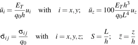
1.1 Leonardo’s description of beam bending [1]. . . 1

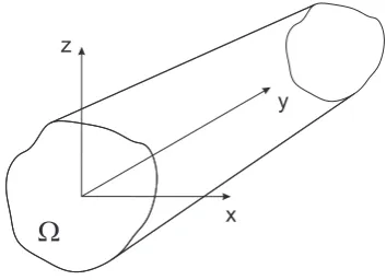
2.1 Adopted coordinate system. . . 9

2.2 Differences between Euler-Bernoulli and Timoshenko beam theories. . . . 10

2.3 Homogeneous condition of transverse stress components at the unloaded edges of the beam. . . 11

2.4 Rigid torsion of the beam cross-section. . . 13

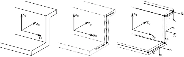
2.5 GBT approximation, global,()g, and local,()L, reference systems. . . 14

3.1 Coordinate system and fiber orientation angle. . . 21

3.2 Cross-section L-elements in natural geometry. . . 23

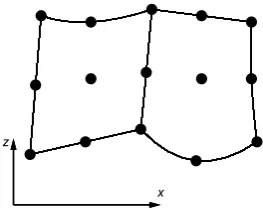
3.3 Two assembled L9 elements in actual geometry. . . 24

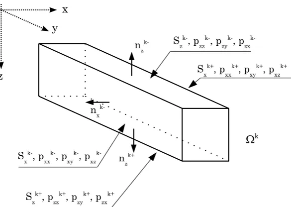
4.1 Components of a surface loading; lateral surfaces and normal vectors of the beam. . . 29

4.2 Components of a line loading. . . 31

4.3 Generalized forces applied at the ends of the beam. . . 32

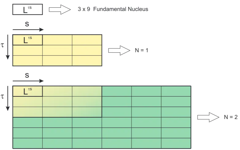
7.1 Expansion of the matrixLτs_{for a given expansion order and TE. . . .} ₅₆

7.2 Boundary conditions of the beam element and sign conventions. . . 62

7.3 Assembly of dynamic stiffness matrices. . . 65

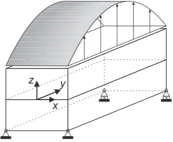
8.1 Simply supported composite beam of two-layer square cross-section sub-jected to sinusoidal pressure load. . . 68

8.2 Distribution of normalized axial displacement ¯uyalong ¯zand at(x,y) = (0,0); simply-supported composite beam under sinusoidal surface loading. . . 70

(15)

8.5 Distribution of normalized axial stress, ¯σzz, along ¯zand at(x,y) = (0,L/2);

simply-supported composite beam under sinusoidal surface loading. . . 72

8.6 Distribution of normalized axial stress, ¯σyz, along ¯z and at (x,y) = (0,0);

8.7 Solid rectangular cross-section. . . 77

8.8 First (a), second (b) and third (c) bending modes for a SS square beam

(L/b=10); DSMN=4 TE model. . . 79

8.9 First bending (a), second bending (b), first torsional (c) and second torsional

(d) modes for a CF square cross-section beam (L/b=10); DSMN=5 TE

model. . . 80

8.10 Cross-section of the thin-walled cylinder. . . 81

8.11 Percentage error between the RBFs and exact DSM solutions for various

expansion orders and boundary conditions; Thin-walled cylinder. . . 83

8.12 First flexural (a), second flexural (b), first shell-like (c), second shell-like (d), first torsional (e) and second torsional (f) modes for a CC thin-walled

cylinder; DSMN=5 TE model. . . 84

8.13 Effect of ply orientation angle on first flexural natural frequencies of

two-layer CF beams; DSMN=4 TE model versus [144]. . . 86

8.14 Effect of material anisotropy on the first flexural natural frequencies of

angle-ply and cross-ply CF beams; DSMN=4 TE model versus [144]. . . 86

8.15 First four modes of the SS-F-SS-F cross-ply plate witha/h=5,N=6. . . 88

8.16 First four modes of the SS-F-SS-F cross-ply plate witha/h=10,N=6. . . 88

8.17 Experimental setup for the measurement of the natural frequencies,

symmet-ric 32-layer plate. . . 90

8.18 First five modes of the FFFF symmetric 32-layer thin plate,N=6. . . 90

8.19 Semi-circular cross-section. . . 91

8.20 Uncoupled (a, b, c) and coupled (d, e, f) modal shapes for the unloaded

(P=0) SS semi-circular beam; DSM-TEN=6 model. . . 95

8.21 First non-dimensional critical buckling load (P_cr∗ = PcrL2

π2EI) versus

length-to-height ratio,L/h, for the rectangular metallic beam. . . 97

8.22 Cross-section of the C-shaped beam. . . 98

8.23 Second flexural-torsional buckling mode of the C-shaped section beam by

the seventh-order (N=7) CUF model. . . 99

(16)

List of Tables

3.1 McLaurin’s polynomials. . . 22

8.1 Maximum non-dimensional transverse displacement, ¯u_z(0,L/2,−h/2), of

the simply-supported composite beam under sinusoidal surface loading. . . 69

8.2 Non-dimensional axial displacement, ¯uy(0,0,−h/2), of the simply-supported

composite beam under sinusoidal surface loading. . . 72

8.3 Non-dimensional axial stress, ¯σyy, at various z coordinates and (x,y) =

(0,L/2); simply-supported composite beam under sinusoidal surface loading. 73

8.4 Non-dimensional transverse normal stress, ¯σzz, at(x,y,z) = (0,L/2,h/2);

8.5 Non-dimensional transverse shear stress, ¯σyz, at (x,y,z) = (0,0,−h/4);

8.6 First to fourth non-dimensional bending frequenciesω∗= ωL

2

b

q

ρ

E for the

SS square beam;L/b=10. . . 78

8.7 Comparison between TE and LE CUF models; non-dimensional natural

frequenciesω∗=ωL

2

b

q

ρ

E for the SS square beam (L/b=10). . . 79

8.8 Non-dimensional natural periods ω∗= ωL

2

b

q

ρ

E for the CF square beam;

L/b=10. . . 80

8.9 Natural frequencies (Hz) of the thin-walled cylinder for different boundary

conditions; Comparison of RBFs and DSM solutions. . . 82

8.10 Non-dimensional natural frequencies, ω∗= ωL

2

b

q

ρ

E11, of a CC [+45/−

45/+45/−45]antisymmetric angle-ply beam. . . 85

8.11 Non-dimensional natural frequencies,ω∗=ωa_h

q

ρ

E2, for the cross-ply

SS-F-SS-F plate. . . 87

8.12 Natural frequencies (Hz) of the FFFF symmetric 32-layer composite thin plate. 89

8.13 Natural frequencies (Hz) for the unloaded (P=0) semi-circular cross-section

(17)

8.14 Natural frequencies (Hz) for the semi-circular cross-section beam undergoing

a compression load (P=1790 N). . . 93

8.15 Natural frequencies (Hz) for the semi-circular cross-section beam undergoing

a traction load (P=−1790 N). . . 94

8.16 First three non-dimensional buckling loads (P_cr∗ = PcrL2

π2EI) of the metallic beam,

L/h=20. . . 96

8.17 First non-dimensional buckling load (P_cr∗ = PcrL2

π2EI) of the metallic beam for

different length-to-height ratiosL/h. . . 97

8.18 Flexural-torsional buckling loads [N] for the axially compressed C-section

beam. . . 98

8.19 Critical buckling loads [MPa] for various length-to-side ratio,L/a, of the SS

square box beam. . . 100

8.20 First four buckling loads [MPa] of the SS square box beam forL/a=100. . 101

8.21 Effect of length-to-height ratio,L/h, on the non-dimensional critical

buck-ling loads (P_cr∗ = PcrL2

E2bh3) of symmetric and anti-symmetric cross-ply SS

lami-nated beams. . . 102

(18)

Nomenclature

Roman Symbols

Bτs ₃_×_{6 fundamental nucleus of the matrix containing the coefficients of the natural}

boundary conditions

˜

C Matrix of the material coefficients

c RBFs shape parameter

D Linear differential operator

F_τ Cross-sectional expansion functions

Kτs ₃_×_{3 fundamental nucleus of the differential stiffness matrix}

Kτs

σyy0 3×3 fundamental nucleus of the differential, geometrical stiffness matrix

Kτsi j ₃_×_{3 fundamental nucleus of the algebraic stiffness matrix due to RBFs collocation}

KKK Dynamic stiffness matrix

L4 Bi-linear Lagrange polynomial expansion

L9 Quadratic Lagrange polynomial expansion

L16 Cubic Lagrange polynomial expansion

L Length of the beam

Lext Work of the external loadings

L_ine Work of the inertial loadings

L_int Strain energy work

L_σ0

(19)

lk Line load vector on the k-th subdomain

Lτs ₃_×_{9 fundamental nucleus of the matrix containing the coefficients of the ordinary}

differential equations

M Number of terms of the expansion

m Number of half-waves along the beam axis

Mτs ₃_×_{3 fundamental nucleus of the mass matrix}

Mτsi j ₃_×_{3 fundamental nucleus of the mass matrix due to RBFs collocation}

N Expansion order of TE models

n Number of centres for RBFs collocation

Π

ΠΠτs 3×3 fundamental nucleus of the differential matrix of the natural boundary conditions

Π ΠΠτs

σyy0 3×3 fundamental nucleus of the differential matrix of the geometrical boundary

conditions

Π

ΠΠτsi j 3×3 fundamental nucleus of the algebraic matrix of the natural boundary conditions

due to RBFs collocation

pk Pressure load vector on the k-th subdomain

pτ

k 3×1 fundamental nucleus of the loading vector

Ps Generalized loads at the end of the beam

q_si Vector of the collocated unknowns

u Displacement vector

uτ Generalized displacement vector

Uτ Vector of the displacements amplitudes

V Beam volume

Greek Symbols

δ Virtual variation

ε

(20)

Nomenclature

φi Radial basis function

ω Angular frequency

Ω Beam cross-section

σσσ Stress vector

σ_yy0 Axial pre-stress

Superscripts and subscripts

i Collocation index of the variable

j Collocation index of the variation

s Expansion index of the variable

τ Expansion index of the variation

Acronyms / Abbreviations

BLWT Beam Layer-Wise Theory

CLPT Classical Lamination Plate Theory

CUF Carrera Unified Formulation

DOFs Degrees of Freedom

DSM Dynamic Stiffness Method

DSV De Saint-Venant

EBBM Euler-Bernoulli Beam Model

ESCBP Exact Solution for the Cylindrical Bending of Plates

FEM Finite Element Method

FSDT First order Shear Deformation Theory

GBT Generalized Beam Theory

HSDT Higher order Shear Deformation Theory

(21)

LTSDT Layer-wise Trigonometric Shear Deformation Theory

ODEs Ordinary Differential Equations

PVW Principle of Virtual Work

RBFs Radial Basis Functions

PGD Proper Generalized Decomposition

TBM Timoshenko Beam Model

TE Taylor Expansion

VABS Variational Asymptotic Beam Sectional Analysis

(22)

Chapter 1 Introduction

1.1 One-dimensional structural theories

Beam models have been developed and exploited extensively over the last several decades for structural analysis of slender bodies, such as columns, arches, helicopter and turbine blades, aircraft wings and bridges amongst others. These models reduce the three-dimensional (3D) problem into a set of one-dimensional (1D) variables, which depend only on the beam-axis coordinate. Clearly, 1D structural theories, or beam theories, are simpler and computationally more efficient than 2D (plate/shell) theories or 3D (solid) elasticity solutions. This simple feature makes beams still very appealing for static and dynamic analyses of structures.

Over the years, many beam models have been developed using different approaches. The main contributions made to the development of the beam theories are outlined in this chapter by referring to different categories depending on the levels of complexity involved. Each category is then described in detail in the subsequent chapters of this thesis.

[image:22.595.217.389.646.710.2]

The first known description of the mechanical behavior of a beam under bending was given by Leonardo da Vinci. In his Madrid Codex [1], Leonardo correctly described the bending behavior of a slender beam, as shown in Fig. 1.1. He hypothesized the well-known linear distribution of the axial strain on the cross-section.

(23)

The classical, oldest and most frequently employed beam models are those by Bernoulli [2] and Euler [3], hereafter referred to as Euler-Bermoulli Beam Model (EBBM), de Saint Venant [4] (DSV) and Timoshenko Beam Model [5, 6] (TBM). These theories share many important features but they also have some important differences. A comprehensive compari-son of EBBM and TBM can be found in [7] and in Chapter 2 of this thesis. In essence, TBM enhances EBBM and DSV by considering the rotatory inertia and shear deformation effects. However, TBM considers only a uniform shear distribution through the cross-section of the beam. It is well-known that a more appropriate distribution should at least be parabolic in order to accommodate the zero stress boundary conditions on the free edges of the beam. Shear correction factors related to the cross-sectional geometry are commonly employed as remedies to compensate for the zero shear condition at the boundaries. While EBBM and DSV are reliable tools for the analysis of homogenous, compact, isotropic slender beam structures under bending, TBM can be employed for moderately thick orthotropic or isotropic beams.

Classical beam theories represent a computationally cheap and, to some extent, reliable tool for many structural mechanics problems. These models are essentially based on a linear axial, out-of-plane displacement field and a constant transverse, in-plane displacement field. In other words, these models can predict linear axial strain distributions and rigid transverse displacements. Although this simplified displacement field requires no more than five degrees of freedom (DOFs), it also precludes the possibility of detecting many important effects, such as out-of-plane warping, in-plane distortions, torsion, coupling effects, or some other local effects. These additional phenomena usually occur due to small slenderness ratios, thin walls, geometrical and mechanical asymmetries, and the anisotropy of the material.

Many methods have been proposed to overcome the above limitations of classical beam theories so as to allow the application of 1D models to any geometry or boundary conditions, without jeopardizing their computational efficiency when compared to 2D and 3D models. Several examples of these models can be found in well known books on the theory of elasticity, for example, the book by Novozhilov [8]. A possible and modern grouping of all these methodologies to build higher-order beam models could be made as follows:

• The introduction of shear correction factors.

• Inclusion of warping functions.

• Saint-Venant based 3D solutions and the implementation of the Proper Generalized Decomposition (PGD) method.

(24)

1.1 One-dimensional structural theories

• The Generalized Beam Theory (GBT).

• The Carrera Unified Formulation (CUF).

As previously mentioned, some of the preliminary approaches were based on the intro-duction of shear correction factors to improve the global response of classical beam theories, see Timoshenko [5, 6, 9], Sokolnikoff [10] and Cowper [11].

The introduction of warping functions to improve the displacement field of beams is another well-known strategy that followed. Warping functions were first introduced in the framework of the Saint-Venant torsion problem [10, 12, 13]. Some of the earliest contributions to this approach were those made by Umanskij [14], Vlasov [15] and Benscoter [16].

The Saint-Venant solution has been the theoretical basis of many advanced beam models.

For instance, 3D elasticity equations were reduced to beam-like structures by Ladevéze and his co-workers [17]. Using this approach, a beam model can be built as the sum of a Saint-Venant part and a residual part and then applied to thick beams and thin-walled sections.

The PGD for structural mechanics was first introduced by Ladevéze [18]. It is a useful

tool to reduce the numerical complexity of a 3D problem. Bognetet al. [19, 20] extended

PGD to plate/shell problems, whereas Vidalet al. [21] extended PGD to beams.

The asymptotic method, on the other hand, represents a significant tool to develop

structural models. In the beam model scenario, the works by Berdichevskyet al. [22, 23]

were among the earliest contributions that exploited the VAM. Such initiatives introduced an alternative approach to construct refined beam theories in which a characteristic parameter (e.g. the cross-sectional thickness of a beam) is exploited to build an asymptotic series. The terms that exhibit the same order of magnitude as the parameter are retained. Some valuable contributions on asymptotic methods related to VABS models can be found in [24].

(25)

One of the most recent contributions to beam theories has been developed within the framework of the CUF [34]. The main novelty of CUF models is that the order of the theory is a free parameter, or can be an input of the analysis and it can be chosen using a convergence study. CUF can also be considered as a tool to evaluate the accuracy of any structural model in a unified manner. For a comprehensive review of CUF literature, the readers are referred to [35].

1.2 Numerical methods

In the majority of the literature on 1D-CUF, the Finite Element Method (FEM) has been used to handle arbitrary complex geometries and loading conditions. Closed form solutions of the structural problems discussed in this thesis can be solved in an exact sense only for a limited class of problems. For example, by assuming the beam kinematics such as the ones which satisfy the simply supported boundary conditions and by limiting the analysis to metallic or cross-ply laminated composite structures, exact solution can be achieved. In this way the axial and in-plane displacement fields can be decoupled and the governing equations can be solved analytically.

To obtain quasi type closed-form solutions with arbitrary boundary conditions for eigen-value problems, the Dynamic Stiffness Method (DSM) can be used. DSM has been quite

extensively developed for beam elements by Banerjee [36–40], Banerjeeet al. [41], and

Williams and Wittrick [42]. Plate elements based on DSM were originally formulated by Wittrick [43] and Wittrick and Williams [44]. Recently, DSM has been applied to Mindlin plate assemblies by Boscolo and Banerjee in [45, 46] and to a higher order shear deformation

theory for composite plates by Fazzolariet al. [47, 48]. In these papers, some background

information on the use of DSM can be found.

The DSM is appealing in elastodynamic analysis because, unlike the FEM, it provides the exact solution of the equations of motion of a structure once the initial assumptions on the displacements field have been made. This essentially means that, unlike the FEM and other approximate methods, the model accuracy is not unduly compromised when a small number of elements are used in the analysis. For instance, one single structural element can be used in the DSM to compute any number of natural frequencies to any desired accuracy. Of course, the accuracy of the DSM will be as good as the accuracy of the governing differential equations of the structural element in free vibration. In fact, the exact Dynamic Stiffness (DS) matrix stems from the solution of the governing differential equations.

(26)

1.3 Thesis objectives and outline

of further numerical methodologies to be used for the approximate solution of the strong form governing equations can be of interest. As an example, the use of alternative methods to FEM and DSM for the analysis of structures, such as the meshless methods based on collocation theory with Radial Basis Functions (RBFs), is attractive due to the absence of a mesh and the considerable ease of the collocation techniques. In recent years, RBFs method showed excellent accuracy in the interpolation of data and functions. The RBFs method was first used by Hardy [50, 51] for the interpolation of geographical scattered data and later used by Kansa [52, 53] for the solution of partial differential equations. Afterward, Ferreira successfully applied RBFs to the analysis of beams and plates [54, 55]. RBFs method is appealing because it results either in an algebraic system or in a linear eigenvalue problem depending on the case. However, numerical instabilities may be encountered in this method and they are discussed later in the present work.

In this thesis and in Paganiet al. [56–59], DSM has been extended to 1D-CUF models

for both metallic and generically laminated composite structures. Also, RBFs method is explored as an alternative method for the solution of strong form governing equations for CUF beams (see [60]).

1.3 Thesis objectives and outline

The present work aims at providing differential governing equations in strong form (as opposed to weak form, which represents an integral form of these equations) of 1D refined CUF structural models and their subsequent solutions by various closed-form and numerical methods. A wide range of problems are considered, including static analysis, free vibration analysis, free vibration of axially loaded beams, and linearized buckling analysis of beam-columns. The main novelties of this research are: (i) the explicit expressions of the strong form governing equations of CUF beam theories, especially the equations of motion of axially-loaded beam-columns; (ii) the extension of DSM and RBFs to free vibration and buckling analysis of refined CUF beam theories; and (iii) the exact closed-form benchmark solutions for various structural problems, including analytical layer-wise solutions of laminated beams and plates. The general lay-out of the thesis is as follows:

• Brief bibliographic surveys on classical and refined beam modelling techniques and related solution methods are given in this introductory chapter.

(27)

the additions of terms within the displacement field. Various state-of-the-art approaches are also discussed, including GBT, VAM and asymptotic models.

• In Chapter 3, higher-order beam models are formulated in a unified manner by em-ploying the CUF. Within the framework of CUF, the beam kinematics are written as the generic expansion of the generalized displacements using arbitrary cross-sectional functions. Depending on the choice of the kind and the order of the cross-sectional functions, various beam theories can be formulated. In this thesis, two classes of 1D CUF models are considered. These are namely, the Taylor Expansion (TE) class and the Lagrange Expansion (LE) class.

• The strong form governing equations of the generic, refined beam model are developed in Chapter 4. By using the Principle of Virtual Work (PVW) as variational statement, various problems are addressed by either including or excluding the virtual works due to inertial loadings, external loadings and pre-stress along with the virtual work of the strain energy. According to CUF, the governing equations are written in terms of the fundamental nuclei. These nuclei, given the theory order, can be automatically expanded to obtain the equations of the desired theory.

• In Chapter 5, closed-form analytical solutions are provided by imposing simply sup-ported boundary conditions and limiting the analysis to metallic or cross-ply laminates. Attention is focused on the static and free vibration problems, although the procedure can be extended to other problems.

• The material and boundary condition limitations are overcome in Chapter 6, where a collocation method is formulated by using RBFs to approximate the displacement functions and the corresponding derivatives.

• In Chapter 7 the governing equations are rearranged and the transcendental dynamic stiffness matrix is formulated. By using an iterative procedure, namely the Wittrick and Williams algorithm [49], the non-linear eigenvalue problem is solved.

• Some selective results are discussed in Chapter 8. The attention is mainly focused on the efficiency of both TE and LE models as well as on the accuracy of the proposed numerical methodologies when applied to the analysis of solid and thin-walled cross-section beams. Both metallic and composite beams and plates are addressed.

• The conclusions are finally drawn in Chapters 9 and 10.

(28)

1.3 Thesis objectives and outline

• In Appendix A, the material coefficients and the constitutive relations are discussed in detail.

• Appendix B briefly recalls the resolution technique for a generic system of second order differential equations, which is useful in the DSM formulation.

• An innovative forward/backward Gauss elimination algorithm is devised in Appendix C.

(29)

(30)

Chapter 2 Kinematics of beams

This chapter provides details of some of the most important beam models that have been developed in the last few years and, in most cases, are still being developed. For the sake of brevity, only the main features of each formulation are given and described in order to highlight their advantages and disadvantages. The right-handed Cartesian coordinate system shown in Fig. 2.1 is adopted throughout this thesis.

x z

y

[image:30.595.215.392.413.541.2]

W

Figure 2.1 Adopted coordinate system.

2.1 Classical beam theories

Consider a beam structure under bending in the planexy(see Fig. 2.2). The kinematic field

of EBBM (Euler-Bernoulli Beam Model) can be written as:

u_x=u_x₁ uy=uy1−x

∂ux1

∂y

(31)

∂u x1

∂y x

Deformed configuration

Un-deformed configuration

x

y

f_z= f_zx

u x1

(a) EBBM

∂u

x1 ∂y

f_z f_zx

u

x1 x

(b) TBM

Figure 2.2 Differences between Euler-Bernoulli and Timoshenko beam theories.

whereu_xandu_yare the displacement components of a point belonging to the beam domain

alongxand y, respectively. u_x₁ andu_y₁ are the displacements of the beam axis, whereas

−∂ux1

∂y is the rotation of the cross-section about thez-axis (i.e. φz) as shown in Fig. 2.2a.

According to EBBM, the deformed cross-section remains plane and orthogonal to the beam axis. EBBM neglects the cross-sectional shear deformation. Shear stresses play a very important role in many problems (e.g. short beams, composite structures) and their omission can lead to incorrect results. One may like to generalize Eq. (2.1) and overcome the EBBM assumption of the orthogonality of the cross-section. The improved displacement field leads to the TBM (Timoshenko Beam Model),

ux=ux1 uy=uy1+xφz

(2.2)

TBM constitutes an improvement over EBBM since the cross-section does not necessarily remain perpendicular to the beam axis after deformation and one degree of freedom (i.e. the

unknown rotationφz) is added to the original displacement field (see Fig. 2.2b). Nevertheless,

(32)

2.1 Classical beam theories

x

y

Actual distribution of shear stresses

Shear stress distribution according

to TBM

b/2

Figure 2.3 Homogeneous condition of transverse stress components at the unloaded edges of the beam.

One of the earlier attempts to improve the accuracy of TBM was the adoption of shear correction factors. Shear correction factors have been introduced over the years to enhance classical beam theories by several authors, see for example [5, 6, 9–11]. Shear correction factors can be defined in various ways, and they depend on the problem characteristics to a great extent. Two examples of shear correction factor definitions are given here. Cowper

[11] considered the mean deflection of the cross-section (W), the mean angle of rotation of

the cross-section around the neutral axis (Φ) and the total transverse shear force acting on

the cross-section (Q), using the following integrals.

W = 1

Ω

Z Z

u_xdx dz (2.3)

Φ= 1 I

Z Z

xu_ydx dz (2.4)

Q=

Z Z

σxydx dz (2.5)

whereΩis equal to the cross-section area, andI is the second moment of area of the

cross-section. The shear correction factor, KC, is then calculated by exploiting the following

equation:

∂W

∂y −Φ=

Q

KC_AG (2.6)

whereGis the shear modulus of beam material.

Gruttmann and Wagner [61] adopted the following definition of shear correction or shape factor, which was earlier introduced in [62, 63]:

Z Z

(σ_yx2 +σ_yz2)dx dz= F

2

x

K_xGA+ F_z2

K_zGA (2.7)

In Eq. (2.7) the shear correction factors,K_xGandK_zG, are respectively obtained by imposing

(33)

The shear correction factor can be seen as a nonphysical, but artificial way to overcome

classical beam modelling inconsistency. As shown by Carreraet al. [64], refined beam

models based on higher-order displacement fields do not require shear correction factors.

2.2 Higher-order models

For a complete removal of the inconsistency in Timoshenko’s beam theory and an improve-ment of the accuracy of classical beam theories, one may have to assume an arbitrary number of terms in the displacement field [29]. However, the number and the characteristics of

thesehigher-orderterms should be chosen properly. For example, in order to overcome the

inconsistency of TBM, one can require Eq. (2.2) to have null transverse strain components

(γxy= ∂_∂u_yx +∂_∂u_xy) at x=±b₂ of Fig. 2.3. This leads to a third-order displacement field as

follows, which provides the basis for the well-known Vlasov-Reddy beam theory [15, 65],

u_x=u_x₁

uy=uy1+f1(x)φz+g1(x)

∂ux1

∂y

(2.8)

where f₁(x)andg₁(x)are cubic functions of thexcoordinate. It should be noted that, even

though the model based on Eq. (2.8) has the same number of degrees of freedom as the TBM, it clearly overcomes classical beam theory limitations by postulating a quadratic distribution of transverse stresses on the cross-section of the beam.

However, the above theories are not able to include any kinematics resulting from the application of torsional moments. The simplest way to include torsion consists of considering

a rigid rotation of the cross-section around they-axis (i.e. φy), see Fig. 2.4. The resulting

displacement model is:

u_x=zφy

u_z=−xφy

(2.9)

whereu_zis the displacement component along thez-axis. According to Eq. (2.9), a linear

distribution of transverse displacement components is needed to detect the rigid rotation of the cross-section about the beam axis. Beam models that include second-order shear strain capabilities and torsional components can be obtained by summing all the contributions

discussed above. By considering the deformations also in theyz-plane, one has

ux=ux1+zφy

uy=uy1+f1(x)φz+f2(z)φx+g1(x)

∂ux1

∂y +z

φy

∂y

+g2(z)

∂uz1

∂y −xφy

∂y

uz=uz1−xφy

(34)

2.2 Higher-order models

z

x

f_y f_yz

[image:34.595.229.380.113.205.2]

f_yx

Figure 2.4 Rigid torsion of the beam cross-section.

where f₁(x),g₁(x), f₂(z), andg₂(z)are all cubic functions. For example, in the case of a

rectangular cross-section, the cubic functions from Vlasov’s theory [15] are

f₁(x) =x− 4

3b2x

3_, _g

1(x) =− 4 3b2x

3

f₂(z) =z− 4

3h2z

3_, _g

2(z) =− 4 3h2z

3

(2.11)

wherebandhare the dimensions of the rectangular cross-section along thex- andz-axis,

respectively.

The aforementioned beam model, although an advancement, cannot account for many

other higher-order effects, such as the second-order in-plane deformations of the

cross-section and out-of-plane warping. Many refined beam theories have been proposed over the last decades to overcome these limitations of classical beam modelling and they are briefly discussed in the following sections. As a general guideline, one can state that the richer the kinematic field, the more accurate the 1D model turns out to be [29]. However, a richer displacement field clearly leads to a higher number of equations to be solved. Furthermore, the choice of the additional expansion terms is obviously problem dependent. The most accurate beam models that have been developed in the last few years are now briefly discussed.

2.2.1 Generalized beam theory

(35)

xg

yg

zg

xg

yg

zg

s

xg

yg

zg

xL

yL

zL

xL

yL

zL

xL

yL

[image:35.595.138.444.107.202.2]

zL

Figure 2.5 GBT approximation, global,()g, and local,()L, reference systems.

were proposed by Davies and Leach [67], while refined second-order models were given simultaneously by the same authors in [68]. An extension of GBT to orthotropic materials was proposed by Silvestre and Camotim [28] and Silvestre [69]. The GBT approach, as shown in [28], assumes that the displacement field of a prismatic thin-walled beam (see Fig. 2.5) is a product of two functions as shown below

u(x_g,y_g,z_g) =u(s)ψ(yg) (2.12)

whereu(s)is the mid-wall displacement vector, which depends on the curvilinear coordinate

sgoing around the cross-section (see Fig. 2.5), andψ(yg)is an amplitude function defined

along the beam axis y. Figure 2.5 also shows how, according to GBT, the beam can be

assumed to be composed of a number of panels (see [28]). In its simplest form, GBT states that, for each panel:

• The Kirchhoff’s hypotheses are satisfied (γxy=0,γxz=0 andεxx=0).

• The only membrane (m) strain considered is the longitudinal one, i.e. ε_yym ̸=0. On the

other hand, all the flexural (f) strains are taken into account, i.e. εyyf ̸=0,εzzf ̸=0 and

γyzf ̸=0.

The mid-wall deflection curve can be considered as a piece-wise segment defined by using a

number of nodes (see Fig.2.5). If the generalized displacementsu(s)are assumed to have a

linear behaviour, the GBT kinematics becomes

u(xg,yg,zg) =ukFk(s)ψ(yg) (2.13)

whereF_k(s)is a linear function that is equal to 1 in thek-th node and 0 in the other nodes,

andu_k is the displacement vector in thek-th node. Moreover, GBT introduces a number of

geometrical relations that allow the transverse displacements,uxanduz, to be expressed in

(36)

2.2 Higher-order models

The GBT has been widely used in the analysis of thin-walled structures over the past twenty years. This type of model has been used to solve several structural problems and a few examples are reviewed next. The GBT was applied to dynamic problems in the works by Bebiano [70, 71], in which the global and local modes were investigated. Also, the elastic stability of thin-walled structures has been investigated extensively using the GBT. Schardt [72, 27] used the GBT model to perform the buckling analysis of thin-walled structures. The same approach was used by Goncalves and Camotim [73] to investigate the local and the global buckling of isotropic structures. Other investigators who used the GBT models in

buckling analysis are Diniset al. [74], Silvestre [75] and Basagliaet al. [76] amongst others.

An experimental verification of the GBT for the buckling analysis was provided by Leach and Davies [77]. The capabilities of GBT in the analysis of thin-walled structures and its low computational costs make GBT particularly useful for non-linear analyses. Goncalves and Camotim [78] introduced a non-linear formulation based on GBT to investigate the post-buckling behaviour of thin-walled structures, in which plasticity and inelastic effects

were included. Other non-linear beam models based on GBT were presented by Basagliaet

al. [79] and Abambreset al. [80, 81].

2.2.2 Warping functions

The so-called warping function was originally introduced with the Saint-Venant torsion problem, which has been formulated in many textbooks and papers over the years [10, 12, 13] as a standard procedure in the theory of elasticity. According to the Saint-Venant free warping problem, the warping function is the solution of Laplace’s equation subjected to Neumann boundary conditions [82].

The most well-known theories that account for higher-order phenomena through the

use of the warping function are those by Vlasov [15] and Benscoter [16]. In these theories, non-uniform warping in thin-walled profiles is taken into account by including, in the

displacement field, the following longitudinal warping displacement,uwrpy :

uwrp_y (x,y,z) =Γ(x,z)µ(y) (2.14)

whereyis the longitudinal axis of the beam,xandzare the coordinates of the cross-section,

µ is the warping parameter, andΓis the Saint-Venant warping function, which depends on

the geometry of the cross-section. In the case of a shear-bending problem on thexy-plane,

the warping function is a cubic function of the x-coordinate [83] and µ does not necessarily

(37)

warping parameterµ is the derivative of the rotation angle [15] or it can be an independent

function [16].

The application of the Vlasov beam model to thin-walled beams with a closed cross-section leads to unsatisfactory results, since the mid-plane shear strains in the walls cannot be neglected. One of the earliest investigators to formulate the warping function for closed profiles was Umanskij [14]. From then on, many researchers have developed advanced beam theories based on the use of the Saint-Venant warping function. Some recent important contributions are summarized as follows. El Fatmi [84–86] developed a non-uniform warping theory that accounts for three independent warping parameters and related warping functions. Prokic [87–89] formulated a new warping function that is able to account for both closed and open cross-sections. Sapountzakis and his co-workers developed a boundary element method that includes the warping DOF (Degree of Freedom) for non-uniform torsional dynamic [90, 91] and static [92–94] analyses. Wackerfub and Gruttmann [95] developed a Finite Element (Finite Element) based on the Hu-Washizu variational formulation and focussing on the construction of ‘locally-defined’ warping functions. In [82, 96], the unknown warping function has been approximated using an isoparametric concept. Prandtl’s membrane analogy and the Saint Venant torsion theory have been used in [97], on the basis of the Vlasov theory, to obtain an approximate Saint Venant warping function for a prismatic thin-walled beam. In [98], the warping functions have been determined iteratively using equilibrium equations along the beam. Yoon and Lee [99] formulated the entire warping displacement field as a combination of the three basic warping functions (one free warping function and two interface warping functions).

2.2.3 3D Solutions based on the Saint-Venant model and the proper

generalized decomposition

Ladevéze and Simmonds [17, 13] and Ladevézeet al. [100] built models for 3D solutions

of beam problems by adding enrichment terms to the Saint Venant solution. In such a framework, the displacement field can be written as

u(x,y,z) =u_SV(x,y,z) +u_NSV(x,y,z) (2.15)

whereu_SV and u_NSV are the Saint-Venant and residual parts of the displacement field,

re-spectively. The u_NSV term, also known as the decaying term, takes into account various

(38)

2.3 Asymptotic methods

Another important contribution to the solution of the 3D elasticity problem is the Proper Generalized Decomposition (PGD), which was introduced by Ladevéze [18]. Given a 3D

problem, PGD decomposes it as the summation ofN 1D and/or 2D functions ( noting thaty

is the axial coordinate of the beam) as follows

u(x,y,z)≈

N

∑

i=1

Ux_i(x)·Uy_i(y)·Uz_i(z) (2.16)

or,

u(x,y,z)≈

N

∑

i=1

Uxz_i (x,z)·Uy_i(y) (2.17)

whereU are the 2D or 1D unknown functions. This decomposition allows one to solve the

3D problem with 2D or 1D complexity. Bognetet al. [19, 20] applied PGD to plate/shell

problems, while Vidalet al.[21] extended PGD to beams.

2.3 Asymptotic methods

So far, refined beam theories derived from axiomatic methods have been discussed. Ax-iomatic theories are developed on the basis of a number of hypotheses that cannot be always mathematically proved [101]. Moreover, another important drawback of axiomatic methods is the lack of information about the accuracy of the approximated theory with respect to the exact 3D solution. In other words, it is not usually possible to evaluate a-priori the accuracy of an axiomatic theory. The difficulty due to this lack of information has to be overcome by engineers who have to evaluate the validity of a theory on the basis of their knowledge and experience.

The asymptotic method is generally seen as a step towards the development of approxi-mate theories with known accuracy with respect to the 3D exact solution (see [102]), which, in the case of beams, is a good method that can approximate the 3D energy though 1D terms with known accuracy.

The Variational Asymptotic Method (VAM) is an interesting proposition that was origi-nally introduced by Berdichevsky [22] in modelling beams. VAM exploits small parameters

of a beam structure, such as the thickness of the cross-section,h. The unknown functions

(e.g. warping) are then expanded in terms ofhas

(39)

The strain energy is then obtained according to this expansion and only the terms of a certain

order with respect tohare retained. The unknown functions, which are asymptotically correct

up to a chosen order ofh, are then obtained by minimizing the strain energy. The solution

to this variational problem can then be found in closed-form for certain cross-sectional geometries and materials only. In order to overcome the limitations of VAM and to be able to deal with anisotropic and non-homogenous materials, as well as arbitrary cross-sections, the Variational Asymptotic Beam Sectional Analysis (VABS) has been developed [24, 103– 106]. Essentially, VABS exploits the FE approach over the beam cross-section to solve the variational problem.

In general, the development of asymptotic theories is more difficult than the development of axiomatic ones. The main advantage of these theories is that they contain all of the terms whose effectiveness is of the same order of magnitude. Moreover, these theories are exact as

(40)

Chapter 3 Carrera Unified Formulation

Whether axiomatic or asymptotic, the accuracy of a structural theory depends very much on the problem to be analysed. One may merge or amalgamate together the beam theories discussed in the previous chapter in order to address a particular problem. For example, a beam model able of addressing shear, twisting and warping can be formulated by combining Eqs. (2.10) and (2.14). Unfortunately, the resulting model may not be suitable for a different problem, e.g., it may not be able to detect in-plane deformations on the beam cross-section.

In this chapter, the Carrera Unified Formulation (CUF) is introduced. In essence, CUF, by employing a index notation, allows the unification of all the theories of structures in one single formula. Subsequently, in the next part of the thesis, CUF will be used in conjunction with variational principles to derive the governing equations for any-order beam model in a concise and general manner.

3.1 Preliminaries

The rectangular Cartesian coordinate system adopted in this thesis has already been shown in Fig. 2.1, together with a schematic beam structure. The cross-section of the beam, which

lies on thexz-plane, is denoted byΩ, whereas the limits ofyare 0≤y≤L. Consider the

transposed displacement vector, which can be expressed as

u(x,y,z;t) =n u_x u_y u_z

oT

(3.1)

The time variable (t) is implied, but omitted in the remaining part of this chapter for clarity

(41)

follows:

σσσ =

n

σyy σxx σzz σxz σyz σxy

oT

εεε=

n

εyy εxx εzz εxz εyz εxy

oT

(3.2)

In the case of small deformations and angles of rotation, the strain-displacement relations are

εεε=Du (3.3)

whereDis the following linear differential operator matrix

D=             0 ∂

∂y 0

∂

∂x 0 0

0 0 ∂

∂z ∂

∂z 0 ∂ ∂x 0 ∂ ∂z ∂ ∂y ∂ ∂y ∂ ∂x 0

            (3.4)

Constitutive laws are now exploited to obtain stress components to give

σ σ

σ =C˜εεε (3.5)

In the case ofmonoclinic material(i.e., material with one single plane of symmetry, which is

thexy-plane in the present analysis) the matrixC˜ is

˜ C=           ˜

C₃₃ C˜₂₃ C˜₁₃ 0 0 C˜₃₆

˜

C₂₃ C˜₂₂ C˜₁₂ 0 0 C˜₂₆

˜

C₁₃ C˜₁₂ C˜₁₁ 0 0 C˜₁₆

0 0 0 C˜₄₄ C˜₄₅ 0

0 0 0 C˜₄₅ C˜₅₅ 0

˜

C₃₆ C˜₂₆ C˜₁₆ 0 0 C˜₆₆

          (3.6)

Note that the the above matrix describes the constitutive relations of a fibre reinforced lamina

with respect to a generic coordinate system(x,y,z)rotated by an angleθ with respect to the

material coordinate system(1,2,3), see Fig. 3.1. In fact, a fibre reinforced lamina exhibits

(42)

3.2 Unified formulation of beams

x

z 1

2

3

y

Figure 3.1 Coordinate system and fiber orientation angle.

are fully characterized by nine elastic coefficients. Therefore, the 13 elastic coefficients ˜

C_{i j}, which are elements of matrixC˜ in Eq. (3.6), can be expressed as functions of the nine

coefficients with respect to the orthotropic axes(1,2,3)and the fibre rotation angleθ. The

explicit expressions for the coefficients ˜C_{i j} are given in Appendix A. It should be stressed that

models with constant and linear distributions of the in-plane displacement components,u_x

andu_z, may require modified material coefficients to overcome the Poisson locking problem,

see [107]. The explicit expressions of the reduced material coefficients are not reported

here, but the readers are referred to the text by Carreraet al. [108], where the details are

given together with a more comprehensive analysis of the effect of Poisson locking and its correction.

3.2 Unified formulation of beams

According to Carrera Unified Formulation (CUF), the generic displacement field of a beam model can be expressed in a compact manner as an expansion in terms of arbitrary functions,

F_τ,

u(x,y,z) =F_τ(x,z)uτ(y), τ =1,2, ...,M (3.7)

whereF_τ are the functions of the coordinatesxandzon the cross-section;u_τ is the vector of

thegeneralized displacements;Mstands for the number of terms used in the expansion; and

the repeated subscript,τ, indicates summation. The choice ofFτ determines the class of the

(43)

3.2.1 Taylor expansion (TE)

Taylor Expansion (TE) 1D CUF models consists of McLaurin series that use the 2D

polyno-mialsxizjas theF_τ basis. Table 3.1 showsM andF_τ as functions of the expansion order,N,

which represents the maximum order of the polynomials used in the expansion.

N M Fτ

0 1 F1=1

1 3 F2=x,F3=z

2 6 F4=x2,F5=xz,F6=z2

3 10 F7=x3,F8=x2z,F9=xz2,F10=z3 ..

. ... ...

N (N+1)(₂N+2) F₍_N2₊_N₊₂₎_/₂=xN,F₍_N2₊_N₊₄₎_/₂=xN−1z,. . .,F_N(N+3)/2=xzN−1,F(N+1)(N+2)/2=zN

Table 3.1 McLaurin’s polynomials.

According to CUF, classical (see Eqs. (2.1) and (2.2)) and higher-order models (e.g., Eqs. (2.10)) consist of particular cases of TE theories. It should be noted that Eqs. (2.1), (2.2),

and (2.9) are degenerated cases of the linear (N=1) TE model, which can be expressed as

u_x=u_x₁+x u_x₂+z u_x₃ u_y=u_y₁+x u_y₂+z u_y₃ u_z=u_z₁+x u_z₂+z u_z₃

(3.8)

where the parameters on the right-hand side (u_x₁, u_y₁, u_z₁, u_x₂, etc.) are the unknown

generalized displacements of the beam axis as functions of they-coordinate. Higher-order

terms can be taken into account according to Eq. (3.7). For instance, the displacement fields

of Eqs. (2.8) and (2.10) can be considered as particular cases of the third-order (N=3) TE

model,

ux=ux1+x ux2+z ux3+x

2_u

x4+xz ux5+z

2_u x6+x

3_u x7+x

2_{z u} x8+xz

2_u x9+z

3_u x10

uy=uy₁+x uy₂+z uy₃+x2uy₄+xz uy₅+z2uy₆+x3uy₇+x2z uy₈+xz2uy₉+z3uy₁₀

uz=uz1+x uz2+z uz3+x

2_u

z4+xz uz5+z

2_u z6+x

3_u z7+x

2_{z u} z8+xz

2_u z9+z

3_u z10

(3.9)

A more comprehensive treatment of the TE CUF models can be found in [108], where

details about the derivation of classical models from the linear (N=1) TE model and various

(44)

3.2 Unified formulation of beams

(-1, 1)

(-1, -1)

(1, 1)

(1, -1)

(-1, 0) (1, 0)

r s

1 2

3 4

(a) Four-point element, L4

(-1, 1)

(-1, -1)

(1, 1)

(1, -1)

(0, 1)

(0, -1)

(-1, 0) (1, 0) (0, 0)

r s

1 2 3

4 5 6 7

8 9

(b) Nine-point element, L9

(-1, 1)

(-1, -1)

(1, 1)

(1, -1) (-.5, -1)

(-1, -.5) (1, -.5)

r s

1 2 3 4 12 13 14 5 11

15 6 16

10 9 8 7

(-1, .5) (1, .5)

(.5, -1) (-.5, -.5) (.5, -.5) (-.5, .5) (.5, .5)

(-.5, 1) (.5, 1)

(c) Sixteen-point element, L16

Figure 3.2 Cross-section L-elements in natural geometry.

3.2.2 Lagrange expansion (LE)

In this work, another CUF class of models has played an important role and it is referred to as the Lagrange Expansion (LE) class. The LE models exploit Lagrange polynomials to build

1D higher-order models; i.e., Lagrange polynomials are used asF_τ cross-sectional functions.

In the current research, three types of cross-sectional polynomial sets have been adopted. These are shown in Fig. 3.2 which are namely, four-point polynomials (L4), nine-point polynomials (L9), and sixteen-point polynomials (L16). The isoparametric formulation is exploited to deal with arbitrarily shaped geometries.

Some aspects of the Lagrange polynomials as interpolation functions can be found in [109]. However, for the sake of completeness, an illustrative example of the interpolation function is given below for the case of an L4 beam model.

F_τ =1

4(1+r rτ)(1+s sτ) τ =1,2,3,4 (3.10)

whererandsvary from−1 to+1, whereasr_τ ands_τ are the coordinates of the four corner

points whose numbering and location in the natural coordinate frame are shown in Fig. 3.2a. In the case of an L9 kinematics, see Fig. 3.2b, the interpolation functions are given by:

F_τ =1₄(r2+r r_τ)(s2+s s_τ) τ =1,3,5,7

F_τ =1₂s2_τ(s2−s s_τ)(1−r2) +1₂r_τ2(r2−r r_τ)(1−s2) τ =2,4,6,8

F_τ = (1−r2)(1−s2) τ =9

(45)

z

[image:45.595.224.356.106.211.2]

x

Figure 3.3 Two assembled L9 elements in actual geometry.

Finally, the L16 polynomials with reference to Fig. 3.2c are as follows:

F_τ_IJ =L_I(r)LJ(s) I,J=1,· · ·,4 (3.12)

where

L₁(r) = 1

16(r−1)(1−9r

2₎ _L

2(r) = 9

16(3r−1)(r 2₋₁₎

L₃(r) = 9

16(3r+1)(1−r

2₎ _L

4(r) = 1

16(r+1)(9r 2₋₁₎

(3.13)

The complete displacement field of a beam model discretized with one single L9 polynomial is given below for illustrative purposes:

u_x=F₁u_x₁+F₂u_x₂+F₃u_x₃+F₄u_x₄+F₅u_x₅+F₆u_x₆+F₇u_x₇+F₈u_x₈+F₉u_x₉ uy=F1uy1+F2uy2+F3uy3+F4uy4+F5uy5+F6uy6+F7uy7+F8uy8+F9uy9

u_z=F₁u_z₁+F₂u_z₂+F₃u_z₃+F₄u_z₄+F₅u_z₅+F₆u_z₆+F₇u_z₇+F₈u_z₈+F₉u_z₉

(3.14)

where u_x₁, ...,u_z₉ are the displacement variables of the problem, and they represent the

(46)

Chapter 4 Governing differential equations

In this chapter, by taking a recourse to the calculus of variations, the governing differential equations of refined beam models are derived. Attention is particularly focussed on static, free vibration and buckling analyses. Using CUF, the governing differential equations are written in a general, but unified and compact manner. Except for free vibration analysis of axially loaded beams, the same equations can be found in [108], where the same problems are addressed by making use of a slightly different notation.

4.1 Principle of virtual work

Consider a system of particles in equilibrium under applied forces and some prescribed

geometrical constraints. The principle of virtual work states thatthe sum of all the virtual

work,δL, done by the internal and external forces existing in the system in any arbitrary

infinitesimal virtual displacements satisfying the prescribed geometrical constraints is zero:

δL=0 (4.1)

An alternative form of the principle of virtual work states that, ifδLvanishes for any arbitrary

(47)

as a whole and provides all these equations. This principle takes the form of minimizing a certain quantity: the potential energy, for example in static problems. It is significant to note that, since a minimum principle is independent of any special reference system, the equations of analytical mechanics hold for any set of coordinates. This allows one to adjust the coordinates employed to the specific nature of each problem [112].

Calculus of variations and analytical1 mechanics are fascinating topics, but important

though they are, details pertaining to the subject are out of the scope of the present work. For further readings, interested readers are referred to [112, 29]. In this thesis, the principle of virtual work is applied mainly to derive the equations of motion of arbitrary higher-order beam models. In general, by considering inertial effects, external loads, and the contribution of an axial pre-stress in the beam structure, Eq. (4.1) can be written as

δL=δLint+δLine−δLext−δLσyy0 =0 (4.2)

whereL_int stands for the strain energy;L_ine is the contribution of the inertial loads;Lextis

the work done by the external loadings;L_σ0

yy is the work done by the axial pre-stressσ

0

yyon

the corresponding non-linear strainε_yynl; andδ stands for the usual virtual variation operator.

In the following sections each of the contributions in the make up of Eq. (4.2) above are considered separately and written in terms of CUF.

4.1.1 Virtual variation of the strain energy

As detailed in [108], the virtual variation of the strain energy is

δLint=

Z

V

δ εεεTσσσdV (4.3)

Equation (4.3) is rewritten using Eqs. (3.3), (3.5) and (3.7). After integrations by parts (see [101]), it becomes

δLint=

Z

L

δuT_τKτsusdy+

h

δuT_τΠΠΠτsus

iy=L

y=0 (4.4)

where Kτs _{is the differential linear stiffness matrix and} _Π_Π_Πτs _{is the matrix of the natural}

boundary conditions in the form of 3×3 fundamental nuclei. The components ofKτs_are

given below in the case of monoclinic material and they are referred to asKτs

(rc), whereris 1_{According to Lanczos [112], the word “analytical” is used here with reference to the mathematical term}

(48)

4.1 Principle of virtual work

the row number (r=1,2,3) andcdenotes the column number (c=1,2,3):

Kτs

(11)=E

22 τ,xs,x+E

44

τ,zs,z+ E

26 τ,xs−E

26 τs,x

∂

∂y−E

66 τs

∂2

∂y2

Kτs

(12)=E

26 τ,xs,x+E

45

τ,zs,z+ E

23 τ,xs−E

66 τs,x

∂

∂y−

E_τ36_s ∂ 2

∂y2

Kτs

(13)=E

12 τ,xs,z+E

44

τ,zs,x+ E

45 τ,zs−E

16 τs,z

∂

∂y

Kτs

(21)=Eτ26,xs,x+E

45

τ,zs,z+ E

66 τ,xs−E

23 τs,x

∂

∂y−E

36 τs

∂2

∂y2

Kτs

(22)=E

66 τ,xs,x+E

55

τ,zs,z+ E

36 τ,xs−E

36 τs,x

∂

∂y−E

33 τs

∂2

∂y2

Kτs

(23)=E

16 τ,xs,z+E

45

τ,zs,x+ E

55 τ,zs−E

13 τs,z

∂

∂y

Kτs

(31)=E

44 τ,xs,z+E

12

τ,zs,x+ E

16 τ,zs−E

45 τs,z

∂

∂y

Kτs

(32)=E

45 τ,xs,z+E

16

τ,zs,x+ E

13 τ,zs−E

55 τs,z

∂

∂y

Kτs

(33)=E

44 τ,xs,x+E

11

τ,zs,z+ E

45 τ,xs−E

45 τs,x

∂

∂y−E

55 τs

∂2

∂y2

(4.5)

The generic termE_τα β_,

θs,ζ above is a cross-sectional moment parameter given by

E_τα β_,

θs,ζ =

Z

Ω

˜

C_{α β}F_τ,_θFs,_ζdΩ (4.6)

where the cross-sectional functionsF_τ have been defined in Chapter 3. The suffix after the

comma in Eq. (4.5) denotes the partial derivatives. As far as the boundary conditions are

(49)

Πτ₍₁₁s ₎=E_τ26_s_,_x+E_τ66_s ∂

∂y, Π

τs

(12)=E

66 τs,x+E

36 τs

∂

∂y, Π

τs

(13)=E

16 τs,z

Πτ₍₂₁s ₎=E_τ23_s_,_x+E_τ36_s ∂

∂y, Π

τs

(22)=E

36 τs,x+E

33 τs

∂

∂y, Π

τs

(23)=E

13 τs,z

Πτ₍₃₁s ₎=E_τ45_s_,_z, Πτ₍₃₂s ₎=E_τ55_s_,_z, Πτ₍₃₃s ₎=E_τ45_s_,_x+E_τ55_s ∂

∂y

(4.7)

It will be shown later that the termΠΠΠτsus represents the generalized reaction forces at the

end of the beam. It is worth to underline that the main property of the fundamental nuclei,

Kτs _and

Π

ΠΠτsin this section, is that their formal mathematical expression does not depend

either on the order of the beam theory or on the geometry of the problem. This aspect will also be discussed more in detail later in the thesis.

4.1.2 Virtual variation of the work done by axial pre-stress

The virtual variation of the work due to the axial pre-stress is given by

δL_σ0 yy =

Z

L

Z

Ω

σ_yy0δ ε_yynldΩ

dy (4.8)

Here, the geometric non-linearities are introduced in the axial strain in the following Green-Lagrange manner:

ε_yynl =1

2(u 2

x,y+u

2

y,y+u

2

z,y) (4.9)

After substituting Eqs. (3.7) and (4.9) into Eq. (4.8) and performing integration by parts, one obtains

δL_σ0

yy =−σ

0

yy

Z

L

δuT_τKτs

σyy0usdy+σ

0

yy

h

δuT_τΠΠΠτs σyy0us

iy=L

y=0 (4.10)

whereKτs

σ_yy0 as given below is the fundamental nucleus of the differential geometric stiffness

matrix.

Kτs

σyy0 =



  

E_τs∂

2

∂y2 0 0

0 E_τ_s ∂2

∂y2 0

0 0 E_τ_s ∂2

∂y2

    (4.11) where

Eτs=

Z

Ω

(50)

[image:50.595.164.457.121.329.2]

4.1 Principle of virtual work

Figure 4.1 Components of a surface loading; lateral surfaces and normal vectors of the beam.

The components ofΠΠΠτs

σyy0 are

ΠΠΠτs σyy0 =



 

E_τ_s ∂

∂y 0 0

0 E_τ_s ∂

∂y 0

0 0 E_τ_s∂

∂y





 (4.13)

4.1.3 Virtual variation of external work

The virtual work done by the external loadings is assumed to be due to a surface loading and

a line loading, see Carreraet al.[108]. The components of a surface loading acting above a

k-th sub-domain of the cross-section are:

pk=n pk_xx± pk_xy± p_xzk± pk_zx± pk_zy± pk_zz±

oT

(4.14)

The components of the surface load are shown in Fig. 4.1. The lateral surfaces n

Sk±

φ :φ =x,z

o

of the beam are defined on the basis of the normal unit vector n

nk±

φ :φ =x,z

o

. A normal

unit vector with the same orientation asxorzaxis identifies a positive lateral surface. The

external virtual work due to the pressure loadingpk is given by

δLext=

δLk_p±

xx+δL

k

p±xy+δL

k

p±xz+δL

k

p±zx+δL

k

p±zy+δL

k p±zz

Strong-form governing equations and solutions for variable kinematic beam theories with practical applications

City, University of London Institutional Repository

Citation

:

This is the accepted version of the paper.

This version of the publication may differ from the final published

version.

Permanent repository link: http://openaccess.city.ac.uk/15963/

Link to published version

:

Copyright and reuse:

City Research Online aims to make research

outputs of City, University of London available to a wider audience.

Copyright and Moral Rights remain with the author(s) and/or copyright

holders. URLs from City Research Online may be freely distributed and

linked to.

Strong-form governing equations and

solutions for variable kinematic beam

theories with practical applications

Alfonso Pagani

School of Mathematics, Computer Sciences and Engineering

City University London

This dissertation is submitted for the degree of

Doctor of Philosophy

Supervisors:

J.R. Banerjee

Acknowledgements

Abstract

Contents

List of Figures

List of Tables

Nomenclature

Chapter 1

Introduction

1.1

One-dimensional structural theories

1.2

Numerical methods

1.3

Thesis objectives and outline

Chapter 2

Kinematics of beams

W

2.1

Classical beam theories

2.2

Higher-order models

2.2.1

Generalized beam theory

2.2.2

Warping functions

2.2.3

3D Solutions based on the Saint-Venant model and the proper

generalized decomposition

∑

∑

2.3

Asymptotic methods

Chapter 3

Carrera Unified Formulation

3.1

Preliminaries

3.2

Unified formulation of beams

3.2.1

Taylor expansion (TE)

3.2.2

Lagrange expansion (LE)

Chapter 4

Governing differential equations

4.1

Principle of virtual work

4.1.1

Virtual variation of the strain energy

4.1.2

Virtual variation of the work done by axial pre-stress

4.1.3

Virtual variation of external work