Modal analysis and experimental research into improved centering-leveling devices

      

City, University of London Institutional Repository

Citation

:

Siaudinyte, L., Kilikevicius, A., Sabaitis, D. and Grattan, K. T. V. (2016). Modal

analysis and experimental research into improved centering-leveling devices. Measurement,

88, pp. 9-17. doi: 10.1016/j.measurement.2016.01.044

This is the accepted version of the paper.

This version of the publication may differ from the final published

version.

Permanent repository link:

http://openaccess.city.ac.uk/15811/

Link to published version

:

http://dx.doi.org/10.1016/j.measurement.2016.01.044

Copyright and reuse:

City Research Online aims to make research

outputs of City, University of London available to a wider audience.

Copyright and Moral Rights remain with the author(s) and/or copyright

holders. URLs from City Research Online may be freely distributed and

linked to.

City Research Online:

http://openaccess.city.ac.uk/

[email protected]

Modal analysis and experimental research into improved

centering–leveling devices

Lauryna Šiaudinyte˙

a,⇑

, Art

uras Kilikevicˇius

b

, Deividas Sabaitis

a

,

Kenneth Thomas Victor Grattan

a,c

a_{Vilnius Gediminas Technical University, Institute of Geodesy, Sauletekio al. 12, LT-10223 Vilnius, Lithuania}

b_{Vilnius Gediminas Technical University, Dept. of Mechanical Engineering, Sauletekio al. 12, LT-10223 Vilnius, Lithuania} c

City Graduate School, City University London, Northampton Square London, EC1V0HB, United Kingdom

a b s t r a c t

Centering–leveling devices are often used together with rotary tables to improve measur-ing process in various fields of metrology. The most important factor of measurement qual-ity – accuracy – is affected by numerous external and internal factors. To ensure the optimum quality of measurements, several factors have to be well known and thus taken into account in the final measurement to minimize their influence. Analysis of structural dynamics provides data on sensitivity as well as an appropriate method to verify the ana-lytical model. The paper deals with an analysis of structural dynamics of a plain structure centering–leveling device by performing appropriate modal analysis. The experimental setup for vibration monitoring and measurement principle underpinning the work is described in the paper. Measurement results of table dynamics as well as a comparison of theoretical and experimental modal shapes are discussed.

1. Introduction

The monitoring of the position of an object is very important while performing a wide range of other mea-surements on the object. Coordinate tables, which come in a wide range of sizes, have been developed to adjust the position of a measured object. Some are produced with small dimensions and are designed to have high sensitivity to the adjustment of the object displacement. However, coordinate tables are designed to adjust the position of measured object only in one plane and this causes some problems in practical measurements if there is a need to set up the devices coaxially or to perform a displacement of the object in a vertical plane.

In order to address these issues, the centering–leveling device developed here and investigated in this work can be implemented in association with other precision measure-ment systems, i.e., it can be attached to a rotary or indexing table with a circular scale on the top of it. One of the advantages of the device is its simplified structure and therefore it simplifies the operational alignment proce-dure. Moreover, the measured object can be adjusted in both horizontal and vertical planes [9,19] which is an important advantage.

2. Means and methods for modal analysis

2.1. Overview of the state-of-the-art modal analysis methods

Although operational modal analysis is often used in the fields of earthquake engineering and structural engi-neering including buildings and other great structures to determine modal parameters under real operational condi-tions[8,12,13], it can also be applied in laboratories for testing the individual devices or various sets of laboratory equipment.

Modal analysis is a process in which the structure is characterized by dynamic features, such as an eigenvalue (resonance) frequency, damping and modal shapes. Most of widely used constructions and machinery are affected by some specific form of fluctuation. To understand the problems and the nature of such fluctuations in different types of construction, it is necessary to evaluate the system resonance frequencies. It is common practice to acquire these data by defining the key modal parameters which leads to a mathematical model of the dynamics in the sys-tem. Such a model consists of the appropriate mode shapes, where each represents a frequency and the modal damping. It is these parameters which provide the dynamic description of the construction.

Modal analysis is categorized into two main sections – classical modal analysis (experimental modal analysis) and operational modal analysis. Of these, classical modal analysis allows the calculation of the frequency response function, based on the measured forces of excitation and the response of the construction. Operational modal analy-sis is based on the measurement of the output signals, including environmental noise and forces as a non-measured input signal[5]. The latter is used when there is a physical construction and controlling of artificial con-struction excitation is complicated or impossible. There are many methods for the application of modal analysis described in literature. One of these – fully automated (operational) modal analysis – was developed to avoid parameters that need to be specified or tuned by the user. This modal analysis produced similar results as in a man-ual analysis. Also, an improved modal analysis for three-dimensional problems using face-based smoothed finite element method is discussed in[10], where the main focus is on the Finite Element Method which is used together with meshfree methods and the generalized gradient smoothing techniques[3,13,14,17].

In every research there are certain circumstances which have to be dealt with while performing an experiment. Therefore, the method and means for modal analysis are chosen depending on measurement object shape, size, material, etc. The nature of the proposed experimental approach is based on the principles of the experimental modal analysis. Observing the performance of the pro-posed experimental approach provides sufficient data to conclude the experimental approach results and therefore, to compare theoretical and experimental mode shapes.

Also, a brief review and analysis of the current state-of-the-art of circular scale measurement research has revealed the key problematic areas to be scale precision,

as well as taking steps to increase measurement effective-ness[9,19].

2.2. The centering–leveling table

To determine the angular position of raster scale grat-ing, the centering–leveling device is very useful when scanning the surface of the scale. Raster scales can be made of glass, plastic, etc. The research undertaken here reports a novel technique, using a standardized Optical Disk[7]as a measuring scale as well as several other issues originating from this idea. Also, the experimental modal analysis per-formed on this novel setup provides essential data for mea-surement accuracy improvement. Most significantly, the positioning of an object (its centering and leveling) which has the highest impact on the accuracy of the measure-ment results is addressed. The research carried out reports on a new centering–leveling precision positioning table for raster scale measurement, which has the following key features:

A main frame (outer ring) on which the rest of the com-ponents are mounted;

A centering–leveling disk (inner ring);

A lower ring allowing mounting of the system on other measuring systems;

Two micro-traverses for centering;

Additional supporting components (springs, spheres and cone-shaped heads) for motion transfer.

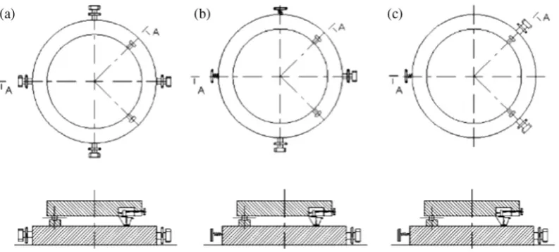
The initial layout for the centering–leveling system, designed to increase the accuracy of the measurements that can be made, is presented inFig. 1.

The position of centering and leveling can be adjusted on the same surface, along two perpendicular axis. The mechanisms for this process are positioned concentrically and the motion is transferred to two supports of the disk. The two mechanisms are specifically positioned to improve the accuracy of the motion and consequently the centering and leveling pitches, using mechanisms that are independent from each other. The centering position is adjusted using two circular elements with a 0.2 mm slope, and to do so this operation includes moving the main cir-cular element. Further, the leveling position is adjusted using two cams with cone-shaped endings mounted on their end. Thus rotating the cams to one side or the other provides the motion required for leveling. The device developed can be easily utilized for other measuring sys-tems to eliminate the type of errors caused by the position of the measured object.

3. Experimental approach

3.1. Modeling and system design

The dynamic parameters of the table can be described by the following formula given by Eq.(1):

½Afq€ðtÞg þ ½Bfq_ðtÞg þ ½CfqðtÞg ¼0 ð1Þ

where (A), (B), (C) are matrices of inertia, damping and stiffness; fqðtÞg;fq_ðtÞg;f€qðtÞg are vectors of velocity and acceleration.

The solution for the above of this phenomenon can be expressed as is shown in Eq.(2):

qðtÞ ¼X

2n

k¼1

zðkÞekkt ð₂Þ

Therefore, the reaction of the system is modal with the base [_z(1). . .z(2n)]. Considering the time momentum, 2n, is

being evaluated, the data are collected in matrix the Q

given by:

[image:4.595.101.498.87.266.2] [image:4.595.71.519.482.701.2]

½qðt1Þ. . .qðt2nÞ |fflfflfflfflfflfflfflfflfflfflfflffl{zfflfflfflfflfflfflfflfflfflfflfflffl}

Q

¼ ½zð1Þ. . .zð2nÞ |fflfflfflfflfflfflfflfflffl{zfflfflfflfflfflfflfflfflffl}

Z

ek1t1 ek1t2n

... .. . ...

ek2nt1 _ek2nt2n

2 66 66 4 3 77 77 5 |fflfflfflfflfflfflfflfflfflfflfflfflfflfflfflfflfflffl{zfflfflfflfflfflfflfflfflfflfflfflfflfflfflfflfflfflffl} K

ð3Þ

Considering the same expression but with a delay of intervalt, it may be expressed by the following:

½qðt1þDtÞ. . .qðt24þDtÞ |fflfflfflfflfflfflfflfflfflfflfflfflfflfflfflfflfflfflfflfflfflfflffl{zfflfflfflfflfflfflfflfflfflfflfflfflfflfflfflfflfflfflfflfflfflfflffl}

QDt

¼ ½zð1Þ. . .zð2nÞ

ek1ðt1þDtÞ _ek1ðt2nþDtÞ

... .. . ...

ek2nðt1þDtÞ _ek2nð2nþDtÞ 2

64

3 75

¼ ½zð1Þek1Dt _z ð2nÞek2nDt

ek1t1 _ek1t2n

... ... ...

ek2nt1 _ek2nt2n 2

64

3 75

¼bzð1Þ. . .bzð2nÞ

|fflfflfflfflfflfflfflfflfflffl{zfflfflfflfflfflfflfflfflfflffl} bz

ek1t1 _ek1t2n

... .. . ...

ek2nt1 _ek2nt2n 2 64 3 75 |fflfflfflfflfflfflfflfflfflfflfflfflfflfflfflfflfflfflffl{zfflfflfflfflfflfflfflfflfflfflfflfflfflfflfflfflfflfflffl} K

ð4Þ

The third reaction of the system, with a delay of inter-val, 2t, is expressed as follows:

qðt1þ2DtÞ...qðt2nþ2DtÞ

½

|fflfflfflfflfflfflfflfflfflfflfflfflfflfflfflfflfflfflfflfflfflfflfflffl{zfflfflfflfflfflfflfflfflfflfflfflfflfflfflfflfflfflfflfflfflfflfflfflffl} Q2Dt

¼ bbzð1Þ...bbzð2nÞ

h i

|fflfflfflfflfflfflfflfflfflffl{zfflfflfflfflfflfflfflfflfflffl} bbz

s

ek1t1 _ek1t2n

... .. . ...

ek2nt1 _ek2nt2n

2 64 3 75 |fflfflfflfflfflfflfflfflfflfflfflfflfflfflfflffl{zfflfflfflfflfflfflfflfflfflfflfflfflfflfflfflffl} K

ð5Þ

Fig. 1.Centering–leveling layouts: (a) centering using four bolts; (b) centering using a pair of bolts and a pair of springs; and (c) centering using a pair of bolts and a single spring.

wherebbzðiÞ¼zðiÞe2kiDt_.

Merging Eqs.(3) and (4)results in:

Q QDt 2 64

3 75¼

Z

b

Z

2 64

3

75

K

ir

U

¼A

K

ð6Þ

In an analogous way, merging Eqs.(4) and (5), results in the following, Eq.(7):

Q_Dt

Q2Dt 2 64

3 75¼

b

Z

bb

Z

2 66 4

3 77

5

K

ir

U

b ¼Ab

K

ð7Þ

Eliminating the matrix between Eqs.(6) and (7)results in the following:

b

UU

1_A¼Ab _ð8Þ

IfA¼ ½a1. . .anandAb¼ ½ba1. . .ban, the expression given

in Eq.(9)provides association between elementsaifrom AtobaifrombA

b

UU

1_a

i¼bai ð9Þ

Additionally, due tobai¼ekiDtai,

b

UU

1_a

i¼ekiDtai ð10Þ

This relationship given in Eq. (10)is expressed as an eigenvalue equation, wheren,the first coordinate of vector

aiis similar to the shape of the construction of Eq.(6). The

eigenvalue allows for equality toekiDt_{, where}k

iis the value

[image:5.595.141.456.87.381.2]

of the complex structure. Eq.(8)reveals that the order of matrices UUb 1 should be equal to double the mode, this acquired by measuring after excitation. To simplify this procedure that is used, the method of least squares for error minimization can be used. It enables more data to

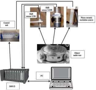
Fig. 3.General overview of the instrumental setup used in this work.

[image:5.595.70.283.539.697.2]

be taken into account by using a greater number of modes.

UandUbare square matrices and therefore the Eq.(10)can be transformed into Eq.(11)as follows:

b

UU

T

h i

UU

T

1

ai¼ekiDtai ð11Þ

3.2. The dynamics of the table

The mechanical instability, influencing the qualitative parameters of the system is next discussed in this research based on modal analysis.

1

₂

3

4

5

6

[image:6.595.99.493.85.610.2]

7

The function of the response to a certain frequency is one of the most effective means of acquiring a frequency-related model of the system. The frequency response func-tion is the spectrum of response, expressed as a spectrum of excitation with a system specific ratio given in Eq.(12):

Xð

_x

Þ ¼Hð

_x

Þ Fð

_x

Þ ð12Þ

The system specific ratioH(

x

) may be expressed as:

Hð

_x

Þ Hð

_x

Þ=Fð

_x

Þ ð13Þ

This describes a complex relation between the excita-tion and response as a funcexcita-tion of frequency

x

. The com-plex ratio leads to introduction of multiplier |H(

x

)| and phase H(

x

) =u(

x

).

From the physical point of view, the response function reveals that the sinusoidal force of excitation with a fre-quency,f, would generate a sinusoidal response force of the same frequency. The amplitude of the response force will be magnified by |H(

x

)|, and the difference between the excitation and response force phases will be equal to

H(

x

). The result response function provides the modal

data, the eigenvalue frequencies and the errors and the damping ratios of the system[4].

3.3. Experimental arrangement and measurements

The key parameters of the system vibration were mea-sured using instrumentation produced by Brüel & Kj

æ

r and this has included:

A Mobile measurement result storing and processing module 3(TYPE 660-D) as shown inFig. 2,

A PC (DELL), as shown inFig. 3,

Shift sensors U20B and U3B (Lion Precision), as shown in Fig. 2c with amplifiers and adapters (Fig. 2a), a piezo-electric excitation source (Fig. 2c) and the inclu-sion of a control unit (Fig. 2b).

A general overview of the instrumental setup used for the determination of the dynamic features is presented in

Fig. 3.

For convenience, portable equipment for the oscillation measuring system control, data processing and measure-ment result storage was used for the experimeasure-ment as this could be readily used in other applications.

4. Results of the investigation

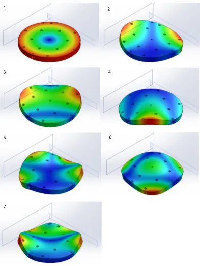
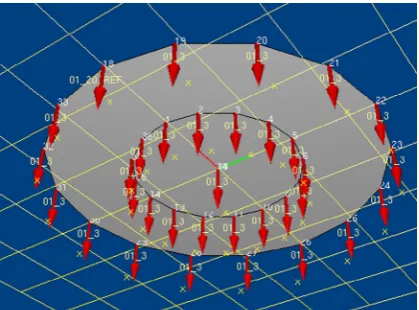
[image:7.595.71.281.90.245.2]

The results of research into the dynamics of the center-ing–leveling device are presented later in this section. However, in order to simulate the most accurate response of the upper plate of centering–leveling device to excita-tion and thus to determine the possible resonant frequen-cies, a finite element method (FEM) analysis was performed[11,16]. In this, the upper plate of centering– leveling device is simulated being divided into finite ele-ments is shown inFig. 4.Fig. 5represents first seven mode shapes of the upper plate of the centering–leveling device. After performing the modal analysis by using the finite element method, seven different modal shapes as well as the correct frequencies and their shifts were determined.

Fig. 6.Measurement points of the centering–leveling device.

Measurement 32 - Response 1 - 16Z-Modal : Measurement 32 : Input : 16Z-Modal TCA 1

400m 800m 1,2 1,6 2 2,4 2,8 3,2 3,6 -6u

-4u -2u 0 2u 4u 6u

[s]

[m] _{Modal : Measurement 32 : Input : Modal TCA 1}Measurement 32 - Response 1 -

16Z-0 100 200 300 400 500 600 700 800 900 1k 0

10n 20n 30n 40n 50n 60n

[Hz] [m]

[image:7.595.81.520.541.707.2]

(a)

(b)

The frequencies determined from the analysis were 298 Hz, 431 Hz, 593 Hz, 1121 Hz, 2312 Hz, 2510 Hz and 2623 Hz for 1, 2, 3, 4, 5, 6 and 7 modal shapes respectively. The measured points for the modal analysis of the center-ing–leveling device are shown inFig. 6.

The structure of the centering–leveling device as well as the improvement of measurement process, thus avoiding harmful working modes which excite oscillations of the device, were determined, based on the research data devel-oped in the model and illustrated inFig. 5.

Measurement 32 - Response 1 - 16Z-Modal : Measurement 32 : Input : 16Z-Modal TCA 1

0 100 200 300 400 500 600 700 800 900 1k

-180 -160 -140 -120

1 2

3

[Hz]

[dB/1,00 m]

[s] (Nominal Values)

Measurement 12 - Response 1 - 30Z-Modal : Measurement 12 : Input : 30Z-Modal TCA 1

0 100 200 300 400 500 600 700 800 900 1k

-180 -160 -140 -120

1 2

3

[Hz]

[dB/1,00 m]

[s] (Nominal Values)

Measurement 28 - Response 1 - 14Z-Modal : Measurement 28 : Input : 14Z-Modal TCA 1

0 100 200 300 400 500 600 700 800 900 1k

-180 -160 -140 -120

1 2

3

[Hz]

[dB/1,00 m]

[s] (Nominal Values)

(a)

(b)

[image:8.595.165.424.85.627.2]

(c)

Fig. 7shows the motion amplitude of the center point of the device under testing and power spectral density of the noise which both show the response to the external excita-tion. The shape of the excitation signal generated by piezo ceramic excitation source by using the swept-sine method is shown inFig. 7wherexaxis represents the time during which the signal was measured andyaxis shows the range of motion of the center point.

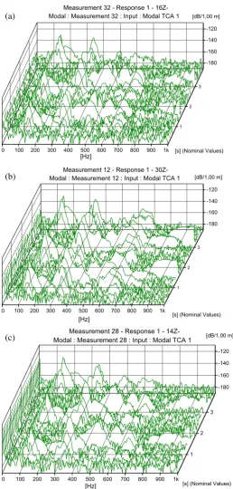
Fig. 8shows a series of 3-D plot of noise spectrum. Here frequency fluctuations that relate both to time and shift amplitudes are displayed.Fig. 8a–c shows greater levels of detail and represents the parameters of center point, inner circle and outer circle of the centering–leveling device respectively.

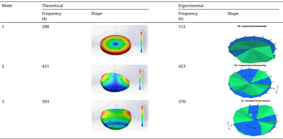
It is inevitable in simulations of this type that minor dif-ferences will appear between the results of the theoretical model and the outputs that represent the experimental data. The comparison between the experimental and the theoretical results is affected by any differences between the actual and the simulated material properties and any imperfections in geometry that may result from the fabri-cation of the device[19,18]. However, it is important to compare both the theoretical and the experimental mode shapes obtained from these two analyses of the center-ing–leveling device.

As shown inFigs. 5 and 8, the dominant frequencies are 312 Hz, 423 Hz and 570 Hz for the first, second and third modes respectively. The biggest portions of the surface of the device are affected by these frequencies and therefore it could have a direct impact on the comparison between the results of actual measurement and of simulation. This comparison is displayed inTable 1. For the figures shown for the experimental work, the green color in the diagrams in theTable 1represents the experimental modal analysis

and shows the deformed surface of the instrument when under test. By contrast, the blue color represents the non-deformed parts of the system geometry. The results of the experimental modal analysis for mode 1 and mode 2 were obtained by using the frequency domain decompo-sition technique and, for mode 3, the stochastic subspace identification technique with unweighted principal com-ponent[15,16].

During the measurement process random errors were unavoidable and an electrical signal was obscured by var-ious sources of noise – shot noise, thermal noise, partition noise, generation–recombination noise, flicker noise, etc.

[6].

5. Conclusion

The research undertaken has enabled data to be obtained from both experimental and theoretical studies of a centering–leveling system and this has showed that shapes, higher than the first mode can be excited in verti-cal plane. Moreover, the comparison of experimental data to that from the theoretical approach yields a very accept-able deviation in the range of 1.9–4.5%. Although the experiment deals with the three first shapes of the table, bounded by 1000 Hz, further research of these frequencies during the operational period should be considered and this is the subject of on-going work.

Acknowledgement

[image:9.595.70.529.106.331.2]

This research was funded by the European Social Fund under the Global Grant measure.

Table 1

Comparison of theoretical and experimental modal analysis.

Mode Theoretical Experimental

Frequency Shape Frequency Shape

Hz Hz

1 298 312

2 431 423

[image:9.595.67.538.108.332.2]

References

[1] R.J. Allemang, A.W. Phillips, The unified matrix polynomial approach to understanding modal parameter estimation: an update, in: Proceedings of the International Seminar on Modal Analysis (ISMA), Leuven, Belgium, 2004.

[2] R.J. Allemang, Experimental modal analysis for vibrating structures. Modal testing and model refinement, in: Proceedings of the Symposium, Boston, MA, November 13–18, 1983 (A84-22613 08-39), American Society of Mechanical Engineers, New York, 1983, pp. 1–29.

[3] R.J. Allemang, D.L. Brown, A.W. Phillips, Survey of modal techniques

applicable to autonomous/semi-autonomous parameter

identification, in: P. Sas, B. Bergen (Eds.), Proceedings of ISMA2010 International Conference on Noise and Vibration Engineering, Leuven, Belgium, September 2010, pp. 3331–3372.

[4]R. Brincker, C. Ventura, Introduction to Operational Modal Analysis, Wiley, New York, 2015. 344 p.

[5]C. Devriendt, G. De Sitter, S. Vanlanduit, P. Guillaume, Operational modal analysis in the presence of harmonic excitations by the use of transmissibility measurements, Mech. Syst. Signal Process. 23 (3) (2009) 621–635.

[6]J.B. Donovan, M.M. Driscoll, Vibration – Induced Phase Noise in Signal Generation Hardware, April 20, EFTF–IFCS Joint Conference, Besancon, France, 2009.

[7] ECMA-364 standard, Data interchange on 120 mm and 80 mm optical disk using +R DL format – capacity: 8.55 and 2.66 Gbytes per Side, third ed. Geneva, 2007 (198 p).

[8]C. Gentile, A. Saisi, Operational modal testing of historic structures at different levels of excitation, Constr. Build. Mater. 48 (2013) 1273– 1285.

[9]V. Giniotis, A. Hope, Measurement and Monitoring, Momentum Press, New York, USA, 2014. 187 p (ISBN 978-1-606-50-379-9). [10]Z. He, G. Li, Z. Zhong, A. Cheng, G. Zhang, E. Li, An improved modal

analysis for three-dimensional problems using face-based smoothed

finite element method, Acta Mechanica Solida Sinica, vol. 26, AMSS Press, Wuhan, China, 2013.

[11]A. Kasparaitis, A. Kilikevicˇius, J. Ve˙zˇys, V. Prokopovic, Dynamic research of angle measurement comparator, J. Vibroeng. 16 (5) (2014) 2287–2296.

[12]A. Kilikevicˇius, V. Vekteris, Diagnostic testing of the comparator carriage vibrations, Ultragarsas (Ultrasound) 2 (59) (2006) 26–30. [13]F. Magalhães, Á. Cunha, Explaining operational modal analysis with

data from an arch bridge, Mech. Syst. Signal Process. 25 (5) (2011) 1431–1450.

[14] T.S. Maung, Hua-Peng Chen, A.M. Alani, Robust dynamic finite element model updating using modal measurements, in: Proceedings of International Conference on Computational Mechanics (CM13), Durham, UK, 2013.

[15]B. Peeters, G. De Roeck, Stochastic system identification for operational modal analysis: a review, J. Dyn. Syst. Meas. Contr. 123 (4) (2001) 659–667.

[16]E. Reynders, System identification methods for (operational) modal analysis: review and comparison, Arch. Comput. Methods Eng. 19 (1) (2012) 51–124.

[17]E. Reynders, J. Houbrechts, G. De Roeck, Fully automated (operational) modal analysis, Mech. Syst. Signal Process. 29 (2012) 228–250.

[18]K. Saeedi, A. Leo, R.B. Bhat, I. Stiharu, Vibration of circular plate with multiple eccentric circular perforations by the Rayleigh–Ritz method, J. Mech. Sci. Technol. 26 (5) (2012) 1439–1448.

[19] L. Siaudinyte, D. Sabaitis, D. Brucas, Assumptions for development of the new centering–leveling device, in: Proceedings of 12th IMEKO TC10 Workshop on Technical Diagnostics New Perspectives in Measurements, Tools and Techniques for Industrial Applications, Florence, Italy, 2013, pp. 50–54.