1
Application of multiple linear regression and Bayesian belief
network approaches to model life risk to beach users in the UK.
Christopher Stokes#a, Gerhard Masselinka, Matthew Revieb, Timothy Scotta, David Purvesb, Thomas Waltersc
a School of Marine Science and Engineering, University of Plymouth, Drake Circus, Plymouth, PL4 8AA, UK.
bDepartment of Management Science, Strathclyde Business School, University of Strathclyde, 199 Cathedral St, Glasgow,
G4 0QU, UK.
c Operations Research Unit, Royal National Lifeboat Institution, West Quay Road, Poole, BH15 1HZ, UK. # Corresponding author email: [email protected] tel: 01752 586177
Abstract
A data-driven, risk-based approach is being pursued by the Royal National Lifeboat Institution (RNLI) to guide the selection of beaches for new lifeguard services around the UK coast. In this contribution, life risk to water-users is quantified from the number and severity of life-threatening incidents at a beach during the peak summer tourist season, and this predictand is modelled using both multiple linear regression and Bayesian belief network approaches. First, the underlying levels of hazard and water-user exposure at each beach were quantified, and a dataset of 77 potential predictor variables was collated at 113 lifeguarded beaches. These data were used to develop exposure and hazard sub-models, and a final prediction of peak-season life risk was made at each beach from the product of the exposure and hazard predictions. Both the regression and Bayesian network algorithms identified that intermediate morphology is associated with increased hazard, while beaches with a slipway were predicted to be less hazardous than those without a slipway. Beaches with increased car parking area and beaches enclosed by headlands were associated with higher water-user numbers by both algorithms, and beach morphology type was seen to either increase water-user numbers (intermediate morphology in the regression model) or decrease water-user numbers (reflective morphology in the Bayesian network). Overall, intermediate beach morphology can be considered the most crucial contributor to water-user life risk, as it was linked to both higher hazard, and higher water-user exposure. The predictive skill of the regression and Bayesian network models are compared, and the benefits that each approach provides to beach risk managers are discussed.
Key Words
Bayesian Network, Multiple linear regression, lifeguard, rip current, beach users
1.
Introduction
risk-2 based approach is being pursued by the RNLI to guide the selection of beaches for new lifeguard units; for this purpose, this paper aims to quantify the level of life risk at UK beaches where incident data are available, and develop a life risk model to inform the roll-out of future lifeguard services.
The Office of the United Nations Disaster Relief Co-ordinator defines risk as “the expected losses from a particular hazard to a specified element at risk in a particular future time period” (Peduzzi et al., 2009). For beach risk management life risk can be defined in terms of the number of people that are exposed to life threatening hazards at a beach, and their vulnerability to those hazards (Kennedy et al., 2013). As a result, a beach with a relatively low hazard level could exhibit a high level of risk if the number of beach users is high, or if the beach users are particularly vulnerable to the hazards present (for example if they have a low competency in the surf-zone environment). In the present study, which examines broad patterns of life threatening, water-related incidents at beaches, vulnerability will be considered homogenous and the conceptual definition of life risk simplifies to:
𝐿𝑖𝑓𝑒 𝑅𝑖𝑠𝑘 = 𝐻𝑎𝑧𝑎𝑟𝑑 ∗ 𝐸𝑥𝑝𝑜𝑠𝑢𝑟𝑒 (1)
Once the three components have been parameterised, the level of life risk, hazard, and exposure at a beach can be estimated from knowledge of the other two factors. Contrary to modelling life risk directly, this approach has the added benefit of enhancing strategic planning, as the mitigation required on a busy beach with few hazards would be different to that required for a quiet but hazardous beach with a similar level of life risk. As lifeguards are primarily concerned with the safety of people in the water, the present study only considers beach water-users, including bathers, swimmers, and surf craft users.
1.1 Water-user hazards
The UK coast is an extremely varied environment. Wave conditions range from oceanic swell to locally generated wind-sea, and mean spring tide ranges vary from 1.5 to 15 m (Scott et al., 2007). The geomorphological settings range from rocky coastline to embayments or open beaches, that can be backed by hard or soft rock cliffs, dunes, or anthropogenic development. These diverse environments pose a variety of hazards to beach water-users, including strong or offshore blowing winds, littoral currents, and tidal cut-off (Scott et al., 2007; 2008). Rocks and reefs pose an obvious hazard to water-users (Mase, 1989), while rocky platforms can expose anglers and beach-goers to deep and/or energetic water and have been attributed to causing an average of 12 drownings per year in Australia (Brighton et al., 2013), although have been studied little in the UK context.
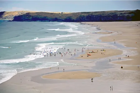
3 Rip currents are often associated with morphological depressions (rip channels) which drive alongshore gradients in wave breaking that generate offshore-directed rip current flows within the channels (Wright and Short, 1984). They are therefore intrinsically linked to the morphological state of the beach. A comparison of beach state observations and lifeguard rescue statistics revealed that some 78% of all incidents that lifeguards attended in the UK between 2005 and 2007 were associated with the intermediate low tide bar/rip and low tide terrace + rip beach states (Scott et al., 2008), which, as their names reveal, both feature conspicuous rip channels.
Fig. 1 RNLI lifeguards monitoring water-users at Perranporth beach, Cornwall, UK. Rip currents can be seen immediately to the left and right of the bathing area, and are revealed by the dark water and reduced wave breaking in the deeper rip channels
1.2 Water-user exposure
4 beach visitors who took part in a study conducted by South West Tourism (2005) were found to travel by car, and the availability of parking and quality of road links are therefore assumed to be influential on beach and water-user numbers.
The proximity of a beach to an urbanised area and the presence of nearby facilities have been found to positively influence people’s choice of beach (Prescient, 2002; South West Tourism, 2005), and Prescient (2002) concluded that people often end up using their closest beach, supporting the notion that beaches near to urbanisation are likely to be busier. However, it is also likely that wild, scenic beaches away from urbanisation appeal to some water-users, as South West Tourism (2005) found that 78% and 98% of their questionnaire respondents decided to visit beaches that weren’t overcrowded, or were in a natural or wild environment, respectively. In either case, the availability of tourist accommodation is likely to have an influence on water-user numbers, and Oxford Economics (2013) indicated that this is more important at rural beaches than at urban beaches, as day-trippers were the majority on urban beaches (44% versus 21% on rural beaches), while people staying overnight were the majority on rural beaches (61% to 39%).
Although the aforementioned questionnaire results may be generalizable in many cases, strictly speaking the results are only relevant to the 4 to 16 different beaches investigated in each study. As beach water-users were not specifically targeted by the studies, other variables were also considered in order to model water-user numbers in the present study. For example, water-users in Wales and Cornwall, UK, have been found to prefer wave conditions of 1-3 m significant height and 10-20 s peak period (Black, 2007; Phillips and House, 2009; Stokes et al., 2014), and three-dimensional, intermediate beach morphology is known to improve surfing amenity (Mead and Black, 2001a; Mead and Black, 2001b; Scarfe et al., 2009) and may also attract higher water-user numbers.
1.3 Structure of paper
Two different approaches were used to model life risk. Multiple linear regression (MLR) was used to separately model hazard and exposure using a selection of independent predictor variables, and a Bayesian belief network (BBN) was developed to provide an alternative model which examines hazard and exposure using Bayesian probability. In each case, the product of the hazard and exposure prediction was used to provide a final prediction of life risk at each beach, as per Eq. 1. Along with expert opinions, the literature described in Sections 1.1 and 1.2 was used to guide the collation of a predictor data set, described in Section 2, to train the models. In section 3 the results of the developed regression and Bayesian network models are presented. In Section 4, the comparative skill and merits of each modelling approach are considered and their application to the modelling of beach life risk is discussed.
2.
Materials and Methods
5 Conservation Society’s ‘Good Beach Guide’ (www.goodbeachguide.co.uk/), The Department for Environment, Food and Rural Affairs’ list of Designated Bathing Waters (www.gov.uk/government/collections/bathing-waters), and the RNLI’s database of lifeguarded and risk-assessed beaches. 1484 individually recognised beaches were identified, and at each beach varying types and amounts of environmental, social, geographical, and safety related data were available. The Good Beach Guide provided information on physical beach characteristics, amenities, and facilities; the RNLI’s United Kingdom Beach Safety Assessment Model (UKBSAM) provided physical and environmental beach variables; and observations of beach user numbers and incidents were provided by RNLI lifeguard and lifeboat data. Geographical and environmental data were also collected from a number of Graphical Information System (GIS) data layers, or were manually digitised from satellite imagery using a GIS platform. As the peak summer season is of key interest to lifeguard managers and provides the greatest availability of lifeguard daily-logs, all temporally varying data used in this study were averaged across the months of July and August.
2.1 Quantification of hazard, exposure, and life risk
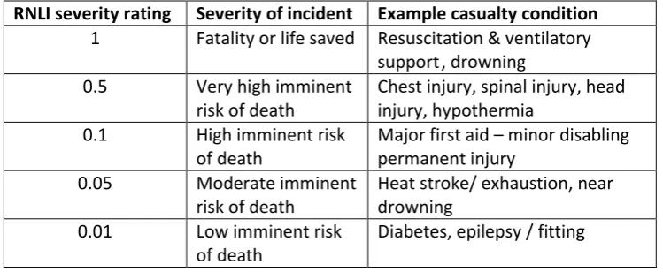
[image:5.595.111.486.613.767.2]To quantify the level of life risk at each beach, the severity values (defined below) assigned to each incident that occurred over the peak summer tourist season at that beach were summed. Incident data came from three different sources: lifeguard logs, lifeboat return-of-service (ROS) data, and the UK’s WAter-Incident Database (WAID). Incident severity is quantified by the RNLI using an incident severity scale, which ranks the potential or actual severity of each incident attended by RNLI lifeguards or lifeboat crews from 0 to 1. A severity of 0 indicates no imminent risk and a severity of 1 is equivalent to a fatality or a life saved (Table 1). As modelling ‘life risk’, rather than ‘injury risk’, is the priority for this particular study, incidents with a severity of 0.1 or less were disregarded from the analysis, meaning that only the most severe incidents - those with at least a ‘very high imminent risk of death’ - were considered. Incidents were assigned to each beach either by a lifeguard logging the incident at that beach, or by the incident having occurred within a 1 km radius of the closest beach’s given coordinates in the case of the ROS and WAID data. For each beach, life risk was calculated as the sum of such severities averaged by the number of years of available incident data, as some beaches have more years of data than others. The incidents considered were water or environmentally related, and did not include socially driven incidents such as violence or self-harm, incidents involving powered water craft, or falls from cliffs.
Table 1 RNLI Incident severity ratings and examples of the potential or actual casualty condition associated to that severity
RNLI severity rating Severity of incident Example casualty condition 1 Fatality or life saved Resuscitation & ventilatory
support , drowning 0.5 Very high imminent
risk of death
Chest injury, spinal injury, head injury, hypothermia
0.1 High imminent risk of death
Major first aid – minor disabling permanent injury
0.05 Moderate imminent risk of death
Heat stroke/ exhaustion, near drowning
0.01 Low imminent risk of death
6 0.00001 Very minor first aid Weaver fish, small cut,
reassurance only
To quantify the level of exposure at each beach, the number of water-users during typical lifeguard operating hours (10 am till 6 pm) in the peak season was examined. The data came from bi-hourly head counts made by RNLI lifeguards, which were recorded in their daily logs. The data represent snapshot estimates of the number of people in the water (including bathers, swimmers, and surf craft users) at any given moment during lifeguarding hours, but do not represent the daily number of water-users as this requires knowledge of how individuals come and go from the water which is impractical to quantify. The head counts have been validated in previous research and were found to provide statistically comparable estimates of water-user numbers to head counts made independently (Cottrell, 2003). As the RNLI wishes to quantify the exposure on a typical busy day, the lifeguard head count data were averaged across bi-hourly observations made on the busiest 1/3rd of days. This therefore provided a single representative value for the exposure level at each beach, considering only the busy peak season days of greatest interest to the RNLI. This exposure predictand will be referred to in the models as the In-Water Population (IWP).
To estimate the underlying level of hazard at each beach, the life risk value was divided by the exposure, indicating the relative probability of a severe incident per water-user. The hazard level therefore attempts to capture the frequency and magnitude of incidents at a beach, but normalises by the exposure to account for beaches which have more water-users but are not necessarily more hazardous. This predictand will be referred to in the models as the Normalised Summed Incident Severity (NSIS). This parameterisation assumes a linear relationship between risk and exposure, presupposing that for a given beach the hazard level stays the same for all exposure levels, although this may not actually be the case. There may also be interaction issues that are not accounted for, for example if hazard were to be higher on busy rural beaches than at busy urbanised beaches. It is therefore acknowledged that there may be systematic skew in the hazard values as a result of this parameterisation.
7 2.2 Predictor variables
A total of 77 predictor variables (listed in Appendix A), consisting of 22 continuous and 55 binary variables, were considered for inclusion in the exposure and hazard models and are briefly summarised as follows:
Proximity to urbanisation, parking, and transport
Spatial variables including urbanised area and car parking area were gathered from GIS data layers (for example the Ordnance Survey’s Meridian 2 database) or were manually digitised from satellite imagery in a GIS platform. A manually nominated coordinate was assigned to each beach near the main beach access point, to enable proximities to be determined. Cleanliness and quality of the beach environment
Designated bathing water status was used as a proxy for environmental quality, as it can only be achieved by beaches that pass annual water quality checks.
Seasonal environmental conditions
Mean wave height, period, and tide range were provided by the UKBSAM. Mean sea surface and air temperatures were obtained from National Oceanic and Atmospheric Administration (NOAA) Odyssea satellite measurements, and Met Office data, respectively.
Geographical characteristics
Information on modal beach morphology, littoral material, beach size, geology, and man-made structures were provided by the UKBSAM and the Good Beach Guide.
Amenities and facilities
Binary variables indicating the availability of beach activities, food, and shops were provided by the Good Beach Guide.
8
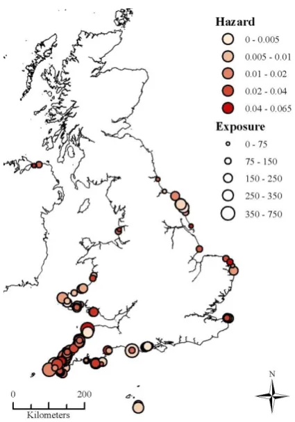
Fig. 2 Hazard level (symbol colour) and exposure level (symbol size) at the 113 model training beaches
2.3 Regression model
A forward and backward stepwise regression algorithm was used to select subsets of variables that had a significant relationship with the hazard and exposure predictand variables. This was chosen as it is a common, off-the-shelf approach to modelling and exploring datasets where many potential predictors are available. The data were pre-processed for the regression in two ways: Firstly, the hazard and exposure predictand variables were log transformed prior to analysis, to satisfy the assumption of normally distributed errors and secondly, inter-correlated predictor variables were removed to yield a set of independent predictors, as collinearity complicates the interpretation of regression estimates (Mason and Perreault Jr, 1991). For any two predictors that were strongly correlated, with a Pearson correlation coefficient R ≥ 0.6, the predictor with the weaker correlation to the predictand was dropped from further analysis. Having removed these initial collinear predictors, the Variance Inflation Factor (Marquardt, 1970) was then assessed to indicate if any of the remaining predictors were significantly dependent on linear combinations of the other predictors. Further removal of variables was undertaken if the Variance Inflation Factor exceeded 10 for any single predictor.
2.4 Bayesian belief network
9 connected nodes. For those wanting a deeper understanding of BBN, we recommend Pearl (1988), Lauritzen (1996), Cowell et al (1999) and, in particular, Jensen (1999). A key feature of BBNs is that they can be developed using expert judgement when data are sparse (Roelen et al., 2003; Qazi et al., 2015), or using machine learning algorithms when data are plentiful (Kafai and Bhanu, 2012), or a mixture of both data and expert input (Bandyopadhyay et al., 2015). Where data are sparse, expert judgement can be used to encode experience. Where data are available, the purpose of constructing a BBN is typically to identify the associations between variables and assess the strength of the identified dependencies. From a modelling perspective, there are different reasons why we would use each approach to developing a BBN. In some situations, we may have no observations and so may wish to harness available expert judgement. At the other extreme, we may have observational data for a situation for which either no expert is available or the cognitive burden of eliciting expert judgement is too great. In practice, a mixed-method approach of expert judgement and observed data is often used.
Where data are available, as in the case of this problem, a range of algorithms are available to support structure learning. These algorithms fall into three broad categories: constraint-based, score-based, and hybrid algorithms (Nagarajan et al., 2013). For each category, a plethora of algorithms exist, some of which have been developed in open source software statistical package R (R, 2016) while some have been developed in commercial software such as Hugin (Madsen et al., 2003). For most of these algorithms, it is necessary for the variables to be either all continuous or all discrete. Where datasets contain both continuous and discrete variables, as is often the case in practice, an additional restriction may be placed on the learning process that ensures that discrete variables can only have discrete parents - a constraint which enables the use of efficient inference procedures (Lauritzen and Jensen, 2001; Kjaerulff and Madsen, 2008). This approach was taken in the present study, where a Bayesian belief network of hazard and exposure was constructed using the statistical package R v3.2.4 (R, 2016) and the bnlearn package (Scutari, 2009). The BBN structure was learned from the data using a Tabu greedy search algorithm, without using any domain knowledge to place restrictions upon the edges, or their orientation (for comparability with the stepwise regression).
3.
Results
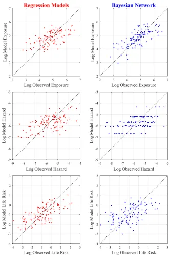
The life risk models generated by the MLR and BBN are described in Sections 3.1 and 3.2, respectively, and their levels of predictive skill are assessed in Section 3.3. Having developed the models, their predictive skill was assessed via a validation phase, using data from beaches previously unseen during the model development. The performance of each model was measured by the root mean squared error (RMSE), the coefficient of determination1 (R2), and Spearman's rank correlation (R
s), between the observed life risk and the model predictions (on the natural log scale). These were evaluated both in-sample, and using 10-fold cross-validation, to examine how each model will perform on an independent dataset to assess any overfitting. 10-fold cross-validation involves the data being randomly divided into 10 partitions; model fitting is then performed using nine-tenths of the data (i.e. 90% of the beaches in the data set), while the remaining one-tenth of the data is retained in order to provide previously unseen data to test the model against. This process is repeated 10 times using a
1 Computed as: 1 − ∑(𝑦 − 𝑓)2/ ∑(𝑦 − 𝑦)2, where 𝑦 = observed values, 𝑓 = predicted values, and 𝑦 = mean of
10 different division of the data set each time, until each division has been used once for validation. The validation from each division is then averaged to produce a single estimate of the model skill, assuming the final model is produced using all of the data.
3.1 Regression models
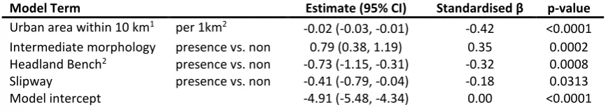
[image:10.595.81.516.467.547.2]The stepwise regression algorithm retained four predictor variables for the hazard sub-model, each of which was significant at the 5% level. Observed and predicted hazard values are plotted in Fig. 3, middle left panel. The model coefficients in Table 2 indicate that hazard was higher at beaches with intermediate morphology, lower at beaches with headland bench geology or a slipway, and decreased as the amount of urbanisation local to the beach increased. The inverse relationship between hazard and urban area can be assumed to be indicative of a demographic effect, whereby a large local population (indicated by a higher urban area) reduces hazard through increased water competency and awareness of coastal hazards. Intermediate morphology is intuitively linked to higher hazard due to its association with rip currents, while slipways may be associated with lower hazard due to typically being located at sheltered beaches with decreased wave energy and currents. It is surprising that headland benches were associated with lower hazard, as they potentially expose beach users to deep and energetic water. A t-test of the difference in mean hazard at beaches with and without headland benches showed no difference in hazard levels. Due to the dependency between headland beaches and other model predictors, particularly urban area and intermediate type, headland benches reduce hazard in the model, rather than intuitively increase it.
Table 2 Regression model with log transformed normalised summed incident severity (hazard level) as the predictand. Effect estimates with 95% confidence intervals, and p-values are reported together with standardised coefficients, to indicate the relative importance of each predictor. To generate the standardised coefficients, the predictand and predictor terms were transformed to have zero means, and standard deviations of one
Model Term Estimate (95% CI) Standardised β p-value
Urban area within 10 km1 per 1km2 -0.02 (-0.03, -0.01) -0.42 <0.0001
Intermediate morphology presence vs. non 0.79 (0.38, 1.19) 0.35 0.0002 Headland Bench2 presence vs. non -0.73 (-1.15, -0.31) -0.32 0.0008
Slipway presence vs. non -0.41 (-0.79, -0.04) -0.18 0.0313
Model intercept -4.91 (-5.48, -4.34) 0.00 <0.0001
1 The amount of urbanised area within a 10 km radius of the chosen beach coordinate
2 Headland bench describes the presence of a rocky platform situated beneath a headland at or around sea level
11
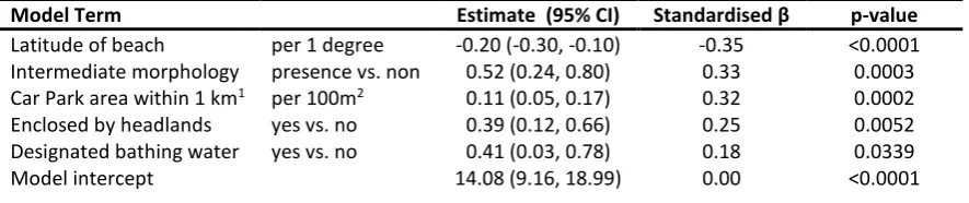
Table 3 Regression model with log transformed in-water population (exposure level) as the predictand. Effect estimates with 95% confidence intervals, and p-values are reported together with standardised coefficients, to indicate the relative importance of each predictor. To generate the standardised coefficients, the predictand and predictor terms were transformed to have zero means, and standard deviations of one
Model Term Estimate (95% CI) Standardised β p-value
Latitude of beach per 1 degree -0.20 (-0.30, -0.10) -0.35 <0.0001 Intermediate morphology presence vs. non 0.52 (0.24, 0.80) 0.33 0.0003 Car Park area within 1 km1 per 100m2 0.11 (0.05, 0.17) 0.32 0.0002
Enclosed by headlands yes vs. no 0.39 (0.12, 0.66) 0.25 0.0052
Designated bathing water yes vs. no 0.41 (0.03, 0.78) 0.18 0.0339
Model intercept 14.08 (9.16, 18.99) 0.00 <0.0001
1 The amount of open-air parking area within a 1 km radius of the chosen beach coordinate
3.2 Bayesian belief network
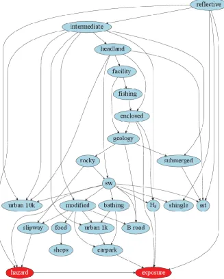
Similar, in part, to the result of the regression model, the BBN (Fig. 4) shows that hazard has direct edges from intermediate beach type and slipway, with an additional association observed with the indicator of a south west beach location. Exposure has direct edges from the enclosed beach, wave height, reflective beach morphology, car parking area, and hazard nodes. Due to the number of interactions, the number of model coefficients is large for a network of this size, so they are omitted for brevity. However, the coefficients show a pattern of increased hazard with intermediate morphology and lower hazard at beaches with a slipway. Population is predicted to increase with car parking area and at enclosed beaches, and decrease with increasing hazard and at reflective (steep) beaches. The effect of south-west location on hazard, and wave height on population, varied depending on the value of the other predictors. Many of these relationships are intuitive and agree with the results of the regression model. However, the link between hazard and population is intriguing, and may indicate a non-linear relationship between the predictands, as exposure and life risk were used to compute the hazard value at each beach. Fig. 4 also indicates potential influences within the holistic system described by our variables. Many of the identified relationships between the predictors are intuitive and logical (such as the influence of urbanised area on car parking area), while some are highly questionable (the influence of reflective beach morphology on sea surface temperature) and result from interdependencies not captured by our model.
3.3 Assessment of model skill
13
14
Fig. 4 The developed Bayesian belief network of beach life risk, showing potential influences between predictor variables (blue) and the hazard and exposure predictands (red). The variables are (from top to bottom and left to right), reflective and intermediate = beach morphology types (binary), headland = headland bench geology (binary), facility = good facilities Vs no facilities (binary), fishing = frequented by anglers (binary), enclosed = beach enclosed by headlands (binary), geology = intertidal rocks present (binary), rocky = rocky outcrops (binary), submerged = submerged at high tide (binary), sw = located in south west UK (binary), urban 10k = urbanised area within 10 km, modified = modified by man-made structures (binary), bathing = designated bathing water (binary), Hs = significant summer wave height, shingle = intertidal shingle
15
Fig. 5 Observed Vs Predicted life risk rank using the combined life risk model (𝒍𝒏(𝐈𝐖𝐏) + 𝒍𝒏(𝐍𝐒𝐈𝐒)) from the regression models (left panel) and the Bayesian belief network (right panel). The Spearman rank correlation for the left and right panels is 0.68 and 0.54, respectively. The beach ranked at number 1 has the highest life risk. The Dashed lines show a 1:1 relationship for reference
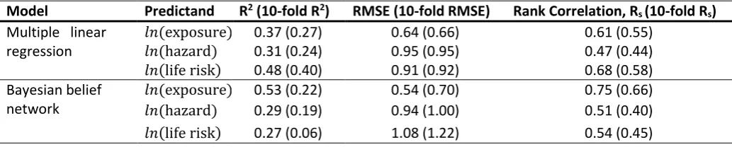
Table 4 Comparison of multiple linear regression and Bayesian belief network model performance. The values in parenthesis are the results of the 10-fold cross validation for each statistic
Model Predictand R2 (10-fold R2) RMSE (10-fold RMSE) Rank Correlation, Rs (10-fold Rs) Multiple linear
regression
𝑙𝑛(exposure) 0.37 (0.27) 0.64 (0.66) 0.61 (0.55) 𝑙𝑛(hazard) 0.31 (0.24) 0.95 (0.95) 0.47 (0.44) 𝑙𝑛(life risk) 0.48 (0.40) 0.91 (0.92) 0.68 (0.58) Bayesian belief
network
[image:15.595.73.590.355.459.2]16
4.
Discussion
Exposure, hazard, and life risk are subject to a plethora of influences, and, as is often the case when modelling human processes, it has not been possible in this study to capture the majority of the variance in each predictand. Additionally, measurement errors in the predictands impart noise and reduce model skill. Exposure level is measured by means of head counts made by lifeguards, and human error is inevitable using this method especially at beaches with large in-water populations (Cottrell, 2003). This source of noise in the exposure data affects the training of both the exposure and hazard models (as exposure is used in the parameterisation of hazard), and therefore has a large overall effect on the prediction of life risk. This could be improved in future studies by collecting automated head count data from camera images (Kammler and Schernewski, 2004; Guillén et al., 2008; Balouin et al., 2014). Hazard and life risk are quantified from incident data collected within 1 km of each beach; in some cases this may result in WAID and ROS incidents being incorrectly assigned to an adjacent beach. There is also subjectivity in the severity rating assigned to each incident, for instance when lifeguard managers have to decide whether an incident is classed as a rescue (severity rating of 0.1) or a life saved (severity rating of 1). Finally, the definition of hazard as the quotient of life risk and exposure is an assumption that may skew the hazard values, as the relationship between the predictands may not be linear as is assumed by this approach.
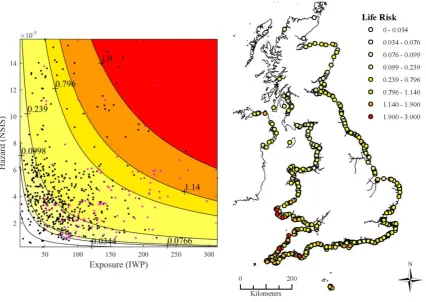
Despite the aforementioned sources of noise in the data, it was possible to capture almost half of the variance in life risk with the regression model, and a quarter of the variance with the Bayesian network. Although these levels of model skill are not sufficient to provide answers to beach management decisions on their own, they do provide a data-driven means with which to aid decision making. For instance, when selecting beaches for future lifeguard services, the predicted life risk ranking, for which both models performed favourably, can be used to narrow down a subset of potentially high-risk beaches, which can then be subjected to a thorough risk assessment process. Fig. 6, right panel, shows life risk predictions from the regression model at 618 UK beaches where sufficient predictor data were available. Beaches where the predicted life risk is high that do not currently have an operational lifeguard service would naturally be the top priority for the RNLI when making further risk assessments and potentially proposing new lifeguard units. Furthermore, the predictions of exposure and hazard in Fig. 6, left panel, can be used to guide different mitigations at beaches with a high exposure but relatively low hazard level, or vice versa.
17 Intermediate beach morphology can be considered the most crucial factor when it comes to water-user life risk, as it was linked to both higher hazard levels, and greater numbers of people in the water.
Fig. 6 Left panel: hazard predictions (NSIS) plotted against exposure predictions (IWP) for 618 UK beaches where predictor data were available. Contours show lines of equal life risk at (from bottom left to top right) the 1, 5, 10, 50, 90 95, and 99 percentile levels. Magenta markers show predictions at the model training beaches. Right panel: life risk predictions for the 618 beaches, plotted at their location in the UK. The same colouring for life risk level is used in the left and right panels
4.1 Comparison of regression and Bayesian network approaches
18 car parking area from the joint probability of its parent nodes. Finally, we could include subjective expert opinions in the BBN modelling, either by creating new variables based on expert judgement, or by modifying the probability distribution between variables.
From Table 3 we see that the predictive power of the BBN is surprisingly poorer than the regression model, and there are a number of potential reasons why this may be the case. The models, as applied, utilise the data in subtly different ways. For example, the BBN minimises error over the entire network rather than focused on a single variable. Different learning algorithms could have been used to focus on individual variables, but we chose not to do this for two reasons: first, as regression is an ‘off-the-shelf’ approach that is widely adopted, we wanted to compare it to the most commonly used BBN algorithms, and second, in this case there were two variables that were of particular interest in the BBN. Other challenges to the BBN emerged due to characteristics in the dataset, for example correlated categorical variables with only two states, coupled with a small dataset, created problems during cross validation. While a larger dataset (i.e. data from more beaches) is ultimately the best solution to this issue, statistical methods exist that could reduce the data requirements for learning the conditional probabilities within the network, and may have improved the CV model skill (for example Prime et al., 2016).
Ultimately, decisions are not taken using a single approach, ignoring information available through other models or expert judgement. Using a complimentary approach, whereby the insight gained from different modelling approaches is likely to be applied in practice. For instance, the regression model could be used when making predictions, while the BBN provides additional understanding of the wider system and added flexibility, such as dealing with missing data and incorporating expert judgement into the process. As such, the two tools complement one another and a mixed-method framework is likely to yield the most useful results. For the RNLI, a mixed-method approach utilising both regression predictions and on site assessments is being utilised in the first instance, with the organisation also trialling the usefulness of Bayesian networks for ongoing analysis of risk on beaches around the UK coast.
4.2 Future research
19
5.
Conclusions
In this contribution, life risk to beach water-user during the peak summer season in the UK has been quantified and modelled at 113 lifeguarded beaches, enabling a beach’s absolute level of life risk or life risk ranking to be predicted with a limited amount of skill. In the process of modelling life risk, the number of water-users (exposure) and the relative probability of a severe incident occurring to a water-user (hazard) at each beach was quantified and modelled, each of which can be used to assist different beach management decisions. A number of variables that have significant relationships with beach exposure and hazard were identified by both the stepwise regression algorithm and the Tabu Bayesian network algorithm. Both models identified that intermediate morphology is associated with increased hazard, while beaches with a slipway were predicted to be less hazardous than those without a slipway. Beaches with increased car parking area and beaches enclosed by headlands were associated with higher water-user numbers by both algorithms, and beach morphology type was seen to either increase water-user numbers (intermediate morphology in the regression model) or decrease water-user numbers (reflective morphology in the Bayesian network). Overall, intermediate beach morphology can be considered the most crucial factor when it comes to water-user life risk, as it was linked to both higher hazard, and higher water-user exposure.
The regression model outperformed the Bayesian network in predictive skill, and was able to capture 48% of the variance in life risk within the training data set. A high level of correlation (R = 0.68) was seen between observed and predicted life risk rankings, and both models are considered to be useful for identifying, or ranking, high risk beaches. Despite the lower in-sample and cross-validation predictive skill of the Bayesian belief network developed here, other Bayesian network manifestations (for instance those that attempt to minimise error on a single predictand) may provide comparable predictive skill to that of a regression model, and would provide other benefits to decision makers that cannot be provided by a regression model. Such benefits include facilitating efficient communication with stakeholders on the different influences and dependencies between variables, handling incomplete datasets or missing observations, and being able to include subjective expert opinions in the modelling where required. In reality, a mixed-method approach utilising both regression and Bayesian networks, as well as expert on-site assessments, may provide the most effective tools for beach risk managers. Due to the availability of training data, the models developed here are potentially weighted towards the characteristics of beaches in south west England and it would therefore be prudent to further calibrate and validate the models as more non south west beach data become available.
Acknowledgements
20
Literature Cited
Austin, M., Scott, T., Brown, J., MacMahan, J., Masselink, G. and Russell, P. 2010. Temporal
observations of rip current circulation on a macrotidal beach. Continental Shelf Research,
30, (9), 1149-1165.
Balouin, Y., Rey-Valette, H. and Picand, P. A. 2014. Automatic assessment and analysis of
beach attendance using video images at the Lido of Sète beach, France. Ocean & Coastal
Management, 102, Part A, 114-122.
Bandyopadhyay, S., Wolfson, J., Vock, D. M., Vazquez-Benitez, G., Adomavicius, G., Elidrisi,
M., Johnson, P. E. and O’Connor, P. J. 2015. Data mining for censored time-to-event data: a
Bayesian network model for predicting cardiovascular risk from electronic health record
data. Data Mining and Knowledge Discovery, 29, (4), 1033-1069.
Black, K. P. 2007. Review of Wave Hub Technical Studies: Impacts on inshore surfing
beaches. ASR Ltd Marine Consulting and Research, Hamilton, New Zealand. 40 pp.
Brander, R. W. 1999. Field observations on the morphodynamic evolution of a low-energy
rip current system. Marine Geology, 157, (3), 199-217.
Brewster, B. C. 2005. Lifesaving and beach safety. In: Schwartz, M. (Ed.). Encyclopedia of
Coastal Science. Springer. pp 589-592. ISBN 1402019033
Brighton, B., Sherker, S., Brander, R., Thompson, M. and Bradstreet, A. 2013. Rip current
related drowning deaths and rescues in Australia 2004–2011. Natural Hazards and Earth
System Science, 13, (4), 1069-1075.
Cottrell, N. 2003. Visitor Population Research. Technical report produced for the Royal
National Lifeboat Institution.
Cowell, R. G., Dawid, A. P., Lauritzen, S. L. and Spiegelhalter, D. J. 1999. Probabilistic
Networks and Expert Systems. Springer, New York.
Greenstreet Berman 2013. Risk assessment and performance measurement research:
Research report. Technical report produced for the Royal National Lifeboat Institution.
21
Hatfield, J., Williamson, A., Sherker, S., Brander, R. and Hayen, A. 2012. Development and
evaluation of an intervention to reduce rip current related beach drowning. Accident
Analysis & Prevention, 46, 45-51.
Howard, R. A. 1990. From Influence to Relevance to Knowledge. In: Oliver, R.M. and Smith,
J.Q. (Eds.). Influence Diagrams, Belief Nets and Decision Analysis. Chichester Wiley. pp 3-23.
Jensen, F. V. 1999. An introduction to Bayesian Belief Networks. UCL Press Limited, London.
Kafai, M. and Bhanu, B. 2012. Dynamic Bayesian networks for vehicle classification in video.
Industrial Informatics, IEEE Transactions on, 8, (1), 100-109.
Kammler, M. and Schernewski, G. 2004. Spatial and temporal analysis of beach tourism
using webcam and aerial photographs. Managing the Baltic Sea. Coastline Reports, 2,
121-128.
Kennedy, D. M., Sherker, S., Brighton, B., Weir, A. and Woodroffe, C. D. 2013. Rocky coast
hazards and public safety: Moving beyond the beach in coastal risk management. Ocean &
Coastal Management, 82, 85-94.
Kjaerulff, U. B. and Madsen, A. L. 2008. Bayesian networks and influence diagrams.
Springer Science+ Business Media, 200, 114.
Lauritzen, S. L. 1996. Graphical Models. Oxford Science Publications, Oxford.
Lauritzen, S. L. and Jensen, F. 2001. Stable local computation with conditional Gaussian
distributions. Statistics and Computing, 11, (2), 191-203.
MacMahan, J., Reniers, A., Brown, J., Brander, R., Thornton, E., Stanton, T., Brown, J. and
Carey, W. 2011. An introduction to rip currents based on field observations. Journal of
Coastal Research, 27, (4), 3-6.
MacMahan, J. H., Thornton, E. B. and Reniers, A. J. 2006. Rip current review. Coastal
Engineering, 53, (2), 191-208.
Madsen, A. L., Lang, M., Kjærulff, U. B. and Jensen, F. 2003. The Hugin tool for learning
Bayesian networks. In: Symbolic and quantitative approaches to reasoning with
22
Marquardt, D. W. 1970. Generalized inverses, ridge regression, biased linear estimation,
and nonlinear estimation. Technometrics, 12, (3), 591-612.
Mase, H. 1989. Random wave runup height on gentle slope. Journal of waterway, port,
coastal, and ocean engineering, 115, (5), 649-661.
Mason, C. H. and Perreault Jr, W. D. 1991. Collinearity, power, and interpretation of
multiple regression analysis. Journal of Marketing research, 268-280.
McKenna, J., Williams, A. T. and Cooper, J. A. G. 2011. Blue Flag or Red Herring: Do beach
awards encourage the public to visit beaches? Tourism Management, 32, (3), 576-588.
Mead, S. and Black, K. 2001a. Field studies leading to the bathymetric classification of
world-class surfing breaks. Journal of Coastal Research, (SI 29), 5-20.
Mead, S. and Black, K. 2001b. Functional component combinations controlling surfing wave
quality at world-class surfing breaks. Journal of Coastal Research, (SI 29), 21-32.
Nagarajan, R., Scutari, M. and Lèbre, S. 2013. Bayesian networks in R. Springer, 122,
125-127.
Oxford Economics 2013. The Economic and Social Benefits of Lifeguard Provision. Technical
report produced for the Royal National Lifeboat Institution.
Pearl, J. 1988. Probabilistic reasoning in intelligent systems: networks of plausible inference.
Morgan Kaufmann, San Fransico, CA.
Peduzzi, P., Dao, H., Herold, C. and Mouton, F. 2009. Assessing global exposure and
vulnerability towards natural hazards: the Disaster Risk Index. Natural Hazards and Earth
System Science, 9, (4), 1149-1159.
Phillips, M. R. and House, C. 2009. An evaluation of priorities for beach tourism: Case
studies from South Wales, UK. Tourism Management, 30, (2), 176-183.
23
Prime, T., Brown, J. M. and Plater, A. J. 2016. Flood inundation uncertainty: The case of a
0.5% annual probability flood event. Environmental Science & Policy, 59, 1-9.
Qazi, A., Quigley, J., Dickson, A. and Gaudenzi, B. 2015. A New Modelling Approach of
Evaluating Preventive and Reactive Strategies for Mitigating Supply Chain Risks. In:
Computational Logistics. Springer. pp 569-585. ISBN 3319242636
R 2016. R: language and environment for statistical computing. R Foundation for Statistical
Computing, Vienna, Austria.
Roelen, A., Wever, R., Cooke, R., Lopuhaä, R., Hale, A. and Goossens, L. 2003. Aviation
causal model using Bayesian Belief Nets to quantify management influence. van Gelder, B.
(Ed.). Safety and Reliability, Swets & Zeitlinger,. Lisse. pp 1315–1320.
Scarfe, B. E., Healy, T. R. and Rennie, H. G. 2009. Research-based surfing literature for
coastal management and the science of surfing-a review. Journal of Coastal Research, 25,
(3), 539-557.
Scott, T., Masselink, G. and Russell, P. 2011. Morphodynamic characteristics and
classification of beaches in England and Wales. Marine Geology, 286, (1-4), 1-20.
Scott, T., Russell, P., Masselink, G., Wooler, A. and Short, A. 2007. Beach rescue statistics
and their relation to nearshore morphology and hazards: a case study for southwest
England. Journal of Coastal Research, 50, 1-6.
Scott, T., Russell, P., Masselink, G., Wooler, A. and Short, A. 2008. High volume sediment
transport and its implications for recreational beach risk. Proceedings 31st International
Conference on Coastal Engineering. ASCE, Hamburg, Germany. pp 4250-4262.
Scutari, M. 2009. Learning Bayesian networks with the bnlearn R package. Journal of
Statistical Software, 35, (3), 1-22.
Short, A. D. 2007. Australian rip systems—friend or foe. Journal of Coastal Research, 50,
7-11.
South West Tourism 2005. South West Bathing Water Study 2005 Final Report. Technical
report produced for the Environment Agency.
24
International Conference on Environmental Interactions of Marine Renewable Energy
Technologies. Stornoway, Isle of Lewis, Outer Hebrides, Scotland.
Wright, L. D. and Short, A. D. 1984. Morphodynamic variability of surf zones and beaches: A
synthesis. Marine Geology, 56, (1–4), 93-118.
Zhang, F. and Wang, X. H. 2013. Assessing preferences of beach users for certain aspects of
weather and ocean conditions: case studies from Australia. International journal of
25
Appendix A. List of potential model predictors
Data Name Data Type Data Source
Facility level = 'none' Binary GBG
Facilities level = 'basic' Binary GBG
Facilities level = 'good' Binary GBG
Facilities level = 'resort' Binary GBG
Swimming Binary GBG
Board Sports Binary GBG
Beach is a Bay Binary GBG
Presence of Shingle Binary GBG
Presence of Rock Binary GBG
Presence of Lifeguards Binary GBG
Presence of Food Vendors Binary GBG
Presence of Toilets Binary GBG
Presence of Shops Binary GBG
Beach in south west England Binary GBG
Designated bathing water Binary GBG
Cleaned by authorities Binary GBG
Distance to Nearest Airport Continuous GIS
Distance to Nearest Train Station Continuous GIS
Distance to Nearest M Road Junction Continuous GIS
Distance to Nearest M Road Continuous GIS
Distance to Nearest A Road Continuous GIS
Distance to Nearest B Road Continuous GIS
Distance to Nearest Minor Road Continuous GIS
Campsite Area Within 1 km Continuous GIS
Carpark Area Within 1 km Continuous GIS
Urban Area Within 1 km Continuous GIS
Urban Area Within 10 km Continuous GIS
Urban Area Within 30 km Continuous GIS
Urban Area Within 60 km Continuous GIS
Mean Summer Sea Surface Temp Within 2 km Continuous GIS
Mean Summer Air Temp Within 2 km Continuous GIS
Latitude Continuous GIS
Longitude Continuous GIS
Campsite Area Within 1km is ≤ 33%ile Binary GIS
Campsite Area Within 1km is > 33%ile and ≤ 66%ile Binary GIS
Campsite Area Within 1km is > 66%ile Binary GIS
Urban Area Within 1km is ≤ 33%ile Binary GIS
Urban Area Within 1km is > 33%ile and ≤ 66%ile Binary GIS
26 Significant Summer Wave Height (mean of highest 1/3rd of wave
heights, Hs) Continuous UKBSAM
Summer wave height (mean of highest 1/10th of wave heights, H
10) Continuous UKBSAM
Mean Summer Wave Period (Tm) Continuous UKBSAM
Mean Spring Tide Range Continuous UKBSAM
Beach Width (dune foot to mean low water level) Continuous UKBSAM
Swell (Tm > 10 s) Binary UKBSAM
Reflective Beach morphology Binary UKBSAM
Intermediate Beach morphology Binary UKBSAM
Dissipative Beach morphology Binary UKBSAM
Enclosed Beach Binary UKBSAM
Submerged at High Tide Binary UKBSAM
Presence of Dunes Binary UKBSAM
Intertidal Geology at High Water Binary UKBSAM
Intertidal Geology at Low Water Binary UKBSAM
Subtidal Geology Binary UKBSAM
High Water Rocks Binary UKBSAM
High Water Boulders Binary UKBSAM
High Water Shingle Binary UKBSAM
High Water Sand Binary UKBSAM
High Water Mud Binary UKBSAM
Intertidal Rocks Binary UKBSAM
Intertidal Boulders Binary UKBSAM
Intertidal Shingle Binary UKBSAM
Intertidal Sand Binary UKBSAM
Intertidal Mud Binary UKBSAM
Presence of an Estuary Binary UKBSAM
Presence of a River Binary UKBSAM
Presence of a Stream Binary UKBSAM
Presence of Groynes Binary UKBSAM
Presence of a Breakwater Binary UKBSAM
Presence of a Pier Binary UKBSAM
Presence of a Slipway Binary UKBSAM
Presence of a Seawall Binary UKBSAM
Presence of a Marina Binary UKBSAM
Seabed Object Binary UKBSAM
Shore Platform Binary UKBSAM
Rock Outcrop Binary UKBSAM