2007
Design and evaluation of a perceptually adaptive
rendering system for immersive virtual reality
environments
Kimberly Ann Weaver Iowa State University
Follow this and additional works at:https://lib.dr.iastate.edu/rtd
Part of theCognitive Psychology Commons, and theComputer Sciences Commons
This Thesis is brought to you for free and open access by the Iowa State University Capstones, Theses and Dissertations at Iowa State University Digital Repository. It has been accepted for inclusion in Retrospective Theses and Dissertations by an authorized administrator of Iowa State University Digital Repository. For more information, please [email protected].
Recommended Citation
Weaver, Kimberly Ann, "Design and evaluation of a perceptually adaptive rendering system for immersive virtual reality environments" (2007).Retrospective Theses and Dissertations. 14895.
by
Kimberly Ann Weaver
A thesis submitted to the graduate faculty
in partial fulfillment of the requirements for the degree of
MASTER OF SCIENCE
Major: Human Computer Interaction
Program of Study Committee: Derrick Parkhurst (Major Professor)
Chris Harding Shana Smith
Iowa State University
Ames, Iowa
2007
1449653
2008
Copyright 2007 by Weaver, Kimberly Ann
UMI Microform
Copyright
All rights reserved. This microform edition is protected against unauthorized copying under Title 17, United States Code.
ProQuest Information and Learning Company 300 North Zeeb Road
P.O. Box 1346
Ann Arbor, MI 48106-1346 All rights reserved.
LIST OF FIGURES ...v
LIST OF TABLES ... vii
ACKNOWLEDGEMENTS ... viii
ABSTRACT ... ix
CHAPTER 1. INTRODUCTION ...1
1.1. Computer Graphics Background ...3
1.1.1. Representing Models as Triangular Meshes ...3
1.1.2. The Graphics Pipeline ...4
1.1.3. Targets for Simplification...7
1.1.4. Representing Geometric Levels of Detail ... 17
1.2. Visual Perception Background ... 20
1.2.1. Anatomy of the Retina ... 20
1.2.2. Attention ... 22
1.2.3. Scene Perception ... 23
1.3. Level of Detail Selection Techniques ... 26
1.3.1. Reactive Level of Detail Selection... 26
1.3.2. Predictive Level of Detail Selection ... 34
1.3.3. Summary... 35
1.4. Immersive Virtual Reality Environments ... 36
1.5. Research Approach ... 38
CHAPTER 2. THE RENDERING SYSTEM ... 41
2.1. Interaction Modes ... 41
2.1.1. Simulation Mode ... 42
2.1.2. Exploration ... 43
2.1.3. Edit ... 44
2.1.4. Experiment... 47
2.2. Level of Detail Selection ... 47
2.2.1. Eccentricity ... 47
2.2.2. Attentional Hysteresis ... 48
2.3. Using Models ... 50
2.3.1. Model Acquisition... 50
2.3.2. Model Simplification ... 50
2.4. XML Scripting ... 51
2.4.1. Master Configuration ... 51
2.4.2. Scene Graph Configuration ... 52
2.4.3. Architecture Configuration ... 53
2.4.4. Light Configuration ... 54
2.4.7. Skeleton Configuration ... 58
2.4.8. Script Configuration ... 58
2.4.9. Level of Detail Schema Configuration... 60
2.5. Code Structure... 62
2.5.1. Command Design Pattern ... 62
2.5.2. The Scene Graph ... 65
2.6. Software Libraries ... 67
2.6.1. VR Juggler ... 67
2.6.2. OpenSG ... 68
2.6.3. Libxml2 ... 69
2.6.4. OPAL and ODE ... 69
2.7. Hardware Description ... 70
CHAPTER 3. PILOT STUDY ... 73
3.1. Methods ... 73
3.1.1. Participants ... 73
3.1.2. Task ... 73
3.1.3. Procedure ... 76
3.1.4. Experimental Design ... 80
3.2. Results ... 83
3.2.1. Visual Acuity ... 83
3.2.2. Simulator Sickness ... 85
3.2.3. Perceptual Measures... 89
3.2.4. Performance Measures ... 94
3.3. Discussion ... 98
CHAPTER 4. FULL STUDY ... 102
4.1. Methods ... 102
4.1.1. Participants ... 102
4.1.2. Task ... 103
4.1.3. Procedure ... 106
4.1.4. Experimental Design ... 108
4.2. Results ... 109
4.2.1. Visual Acuity ... 109
4.2.2. Simulator Sickness ... 111
4.2.3. Qualitative Measures ... 113
4.2.4. Part 1 Quantitative Results ... 113
4.2.5. Part 2 Quantitative Results ... 117
4.3. Discussion ... 121
CHAPTER 5. CONCLUSION ... 124
5.1. Summary ... 124
5.2. Benefit in Older and Newer Systems ... 126
5.3. Clustered Systems ... 127
APPENDIX B. MODELS USED IN THE PILOT AND FULL STUDIES ... 132
APPENDIX C. VISUAL ACUITY QUESTIONNAIRE ... 135
APPENDIX D. SIMULATOR SICKNESS QUESTIONNAIRE... 139
APPENDIX E. POST-TASK QUESTIONNAIRE ... 140
APPENDIX F. END OF STUDY QUESTIONNAIRE ... 141
Figure 1. A Triangle Mesh...4
Figure 2. The Graphics Pipeline ...5
Figure 3. Comparison of Process with Serial Stages versus Parallel Stages ...6
Figure 4. Stanford Bunny rendered as a wireframe at three levels of detail ... 10
Figure 5. Vertex shader code for a wood texture ... 11
Figure 6. Fragment shader code for a wood texture ... 12
Figure 7. Shader simplification ... 14
Figure 8. Simulation Simplification ... 16
Figure 9. Continuous Level of Detail Representation ... 19
Figure 10. View-Dependent LOD Representation ... 20
Figure 11. The Anatomy of the Eye ... 21
Figure 12. Differing Scan Paths by Task ... 25
Figure 13. Top-Down Schematic Representation of Distance-Based LOD Selection ... 27
Figure 14. Implementation of Distance-Based LOD Selection ... 28
Figure 15. Top-Down Schematic Representation of Eccentricity-Based LOD Selection... 29
Figure 16. Implementation of Eccentricity-Based LOD Selection ... 31
Figure 17. Living Room Environment Used by Parkhurst and Niebur ... 39
Figure 18. The 4 Interaction Modes ... 42
Figure 19. Screenshot of the AEST Application... 43
Figure 20. Available Exploration Mode Interactions ... 44
Figure 21. Available Interactions for Edit Mode ... 46
Figure 22. Available Interactions in Experiment Mode ... 47
Figure 23. Top-Down Schematic Representation of Eccentricity-Based Level of Detail ... 48
Figure 24. Structure of the XML Master Configuration File ... 52
Figure 25. Structure of the XML Scene Graph Configuration File ... 55
Figure 26. Structure of the XML Architecture File ... 56
Figure 27. Structure of the XML Light Object File ... 56
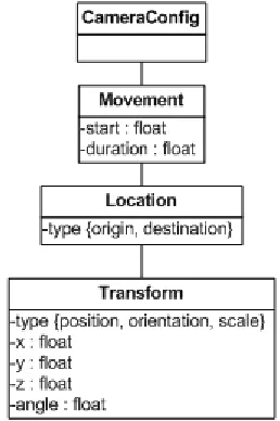
Figure 28. Structure of the XML Camera Configuration File ... 57
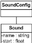
Figure 29. Structure of the XML Sound Configuration File ... 58
Figure 30. Structure of the XML Skeleton Configuration File ... 59
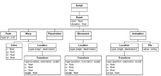
Figure 31. Structure of the XML Script File ... 61
Figure 32. Structure of the XML LOD Schema File... 61
Figure 33. Hierarchy of Control for the Component Managers ... 63
Figure 34. Commands Accepted by the Components in the Rendering System ... 64
Figure 35. Using Scene Time... 65
Figure 36. Scene Graph Diagram ... 67
Figure 37. Rendering of the Original C6 ... 72
Figure 38. Virtual Environment Displayed in the Closed Configuration C4 ... 72
Figure 39. Models Used as Targets in the Pilot Study at Each of Three Levels of Detail ... 75
Figure 40. Visualization of Object Layout in the Virtual Environment ... 79
Figure 41. Top-Down Representation of Eccentricity ... 80
Figure 42. Visual Acuity Scores for Participants in the Pilot Study ... 84
Figure 45. Simulator Sickness Ratings in the Pilot Study Separated by Type ... 88
Figure 46. Frame Rates, Search Times and Distraction Ratings for the Pilot Study. ... 91
Figure 47. Responses to the End-of-the-Study Questionnaire ... 93
Figure 48. Pilot Study Measures Separated by Eccentricity Value ... 96
Figure 49. Pilot Study Measures Separated by Hysteresis Value ... 97
Figure 50. Full Study Dog and Dragon Target Stimuli ... 104
Figure 51. Full Study Monkey and Snail Target Stimuli ... 105
Figure 52. Virtual Environment and Objects Used in the Full Study ... 107
Figure 53. Visual Acuity Reponses from the Full Study... 110
Figure 54. Comparison of Average Simulator Sickness Scores in Part 1 ... 112
Figure 55. Comparison of Average Simulator Sickness Scores in Part 2 ... 112
Figure 56. Search Time, Frame Rates, and Distraction Ratings in Part 1 of the Full Study . 115 Figure 57. Search Distance and Number of Search Errors in Part 1 of the Full Study ... 116
Table 1. Common LOD Representations ... 17
Table 2. Summary of Relevant LOD Research ... 36
Table 3. Experimental Conditions for Participants in the Pilot Study ... 82
Table 4. Example Qualitative Responses to the Conditions in the Pilot Study ... 89
Thank you to the students, staff, and faculty connected with VRAC and the HCI
program for providing advice, support, and friendship over the course of my studies here.
Special thanks to my lab mates in the Human and Computer Vision Lab for feedback on
posters and presentations and more especially for all of the fun we had.
I would like to express my thanks to my major professor, Dr. Derrick Parkhurst. His
ideas, advice and support have been invaluable over the course of my graduate studies and in
particular during the writing of this thesis. Thank you for accepting me as your student, for
looking out for me even when I wasn‟t looking out for myself, and for giving me so many
opportunities to broaden my experience.
Thank you also to my thesis committee members Dr. Chris Harding and Dr. Shana
Smith, as well as to Dr. James Oliver for your valuable feedback and contributions to my
research and this thesis.
I also appreciate the tremendous support from my family. Countless thanks to my
parents who were always available to patiently listen to me ramble. Thank you to my brother
for all of his pragmatic advice on life and grad school. Also, thank you to my sister-in-law
for helping me figure out how to do my statistics even when she had many other things she
ABSTRACT
This thesis presents the design and evaluation of a perceptually adaptive rendering
system for immersive virtual reality. Rendering realistic computer generated scenes can be
computationally intensive. Perceptually adaptive rendering reduces the computational
burden by rendering detail only where it is needed. A rendering system was designed to
employ perceptually adaptive rendering techniques in environments running in immersive
virtual reality. The rendering system combines lessons learned from psychology and
computer science. Eccentricity from the user‟s point of gaze is used to determine when to
render detail in an immersive virtual environment, and when it can be omitted. A pilot study
and a full study were carried out to evaluate the efficacy of the perceptually adaptive
rendering system. The studies showed that frame rates can be improved without overly
distracting the user when an eccentricity-based perceptually adaptive rendering technique is
employed. Perceptually adaptive rendering techniques can be applied in older systems and
CHAPTER 1.
INTRODUCTION
One goal of virtual reality research is to create virtual environments that are
indistinguishable from real environments. We strive for this realism because it can make
people feel more immersed in the environment. They are able to interact with the virtual
environment as if they are interacting with the real world. Creating these near perfect
reproductions of the real world requires processing significant amounts of data and
performing complex calculations very quickly. Objects from nature such as trees are very
difficult to render realistically because there are so many branches and leaves, that the
computer cannot process all of the data fast enough for display. The most realistic lighting
cannot be used in the environment because it takes substantial computational power to
determine the paths of the individual light rays to precisely calculate shadows and reflections.
It is also difficult to calculate with complete accuracy the effect that complex objects have on
each other when colliding because it is necessary to check for collisions against every feature
of an object.
If the environment is too complex, the computer will have to spend a long time
pre-processing and rendering it. As a result, the display will be updated very slowly. The delay
in display rendering increases the lag between when a user initiates an interaction and when
the environment updates to reflect that interaction. If this lag time is too long, the user will
not have a sense of immersion. Any benefit gained from displaying a realistic environment
will be neutralized. Therefore, it is necessary to find a balance between creating a realistic
The balancing act becomes even more pronounced in fully immersive environments
for which large portions of the scene must be rendered simultaneously, or in environments
that are shared over a network where bandwidth becomes a limiting factor. Graphics cards
which perform most of the calculations involved in rendering a realistic virtual environment
are becoming faster. They are capable of handling even larger amounts of data concurrently.
However, this hardware is still insufficient and will be for the foreseeable future. Thus,
computational resources must be managed to ensure the highest quality scene with the least
amount of overhead.
The goal of this research is to manage computational resources by employing
knowledge gained from the study of computer graphics and visual perception to reduce
environment complexity gracefully, without noticeable effects on task performance or
perceived scene quality. This can be done using perceptually adaptive rendering to
determine when to render detail and when to leave detail out based on our understanding of
the limits of human perception. Immersive virtual reality environments require multiple
views of the same scene to be rendered simultaneously, even though the user is unable to see
much of the environment. Even the portion of the scene which is currently visible to the user
can be simplified given that the user only pays attention to a small portion of the scene at any
given time. This can greatly improve rendering update times. Although there are many
different aspects of a virtual environment which can be simplified, this research employs
geometric simplification. Geometric simplification has been around the longest, and
therefore tools are readily available for its implementation in virtual reality environments.
The reduction in geometric complexity decreases the amount of computation and processing
performed in each frame so that the display can be updated quicker. The improvement in
1.1.
Computer Graphics Background
Perceptually adaptive rendering research relies on two aspects of computer graphics.
The first is the method by which models are defined in a three dimensional (3D) graphics
application. The second is the nature of the graphics pipeline. Section 1.1 describes basic
information about these two topics and their relation to perceptually adaptive rendering.
1.1.1. Representing Models as Triangular Meshes
Objects in 3D graphical environments are typically represented as a collection of
vertices and edges that define a surface. Most operations are performed on the vertices. The
graphics processing unit (GPU) of a computer is designed to operate most efficiently when
those vertices are grouped into triangles. These triangles cannot just be arbitrarily provided to
the GPU. In very large models, there could be many triangles sharing a single vertex. With
no organization of triangles, that single vertex would have to be processed many separate
times, leading to inefficiency. Instead, the most common way to represent a 3D model is to
use a triangle mesh. When triangles are arranged into a mesh, a single vertex needs to be
processed only once by the graphics card independent of the number of constituent triangles.
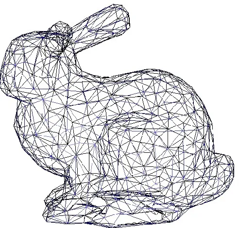
Figure 1 shows a triangle mesh of the Stanford Bunny. The Stanford Bunny is one of the
1.1.2. The Graphics Pipeline
The graphics or rendering pipeline is the set of processes by which a scene composed
of 3D models is transformed into a two-dimensional (2D) image for display.
Figure 2 illustrates the graphics pipeline. The stages are modeling, vertex
manipulation, rasterization, pixel manipulation, and display. First, the modeling stage
involves the representation of an object in 3D space. It also involves associating the object
with any lighting and materials. This is where properties based in simulation interactions are
calculated. For example, if physics is enabled, then the positions of objects as a result of
collisions need to be determined. The first stage of the graphics pipeline is not implemented
[image:15.612.194.440.110.345.2]in the graphics hardware, but instead runs on the central processing unit (CPU).
The remaining stages are processes that occur in the GPU. In the vertex manipulation
stage, the operations that must be performed on each vertex are executed. This can include
lighting and shading, as well as projecting 3D vertices onto a 2D plane. The rasterization
stage is where the 2D vertex information is converted into pixels for display. This involves
taking all of the vertices, transforming them into 2D points, and then filling in the 2D
triangles based on these transformations. During the pixel manipulation stage, the color for
each pixel in the final display is determined. This may be determined by vertex colors and
textures which can be defined along with a model, or more recently by shaders. Shaders are
a set of instructions which the programmer can define to override the normal GPU
calculations. They can be used to calculate more accurate lighting or to add other effects that
can be better represented in 2D space instead of 3D space. After all of the information for a
given pixel is gathered, that pixel is sent to the display device.
Each vertex and the resulting pixels can function as independent entities. The
calculations for any single vertex do not normally depend on the result of operations on
neighboring vertices. The calculations for any single pixel do not normally depend on those
of its neighbors. This means that once a vertex has left a stage in the pipeline, and has
moved onto another stage, another vertex can be pushed into the pipeline. If calculations for
one vertex depended on the results from another vertex, then the computer would have to
completely process a single vertex and render it to the display before it could begin
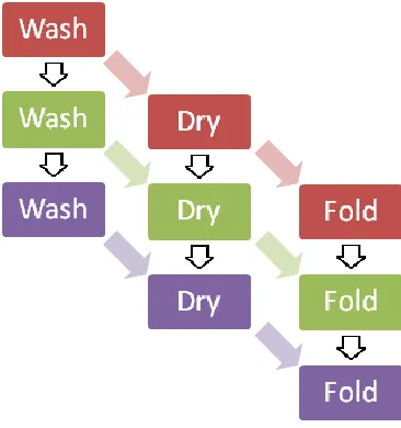
processing the next vertex. This is like washing, drying, and folding a single load of laundry
before starting on a second load of laundry. If you had to do three loads of laundry without
Figure 2. The Graphics Pipeline
any parallel stages, then it would take nine time units to complete all of the loads of laundry.
Because it is possible to start washing the second load of laundry when the first load goes
into dryer, you can speed up the laundry process. When the first load is done drying, you can
put the second load into the dryer, start the third load in the washer, and fold the first load.
Instead of the nine time units required for processing laundry in series, it is possible to
[image:17.612.298.481.306.501.2]processes all three loads of laundry in five steps when stages are performed in parallel.
Figure 3 illustrates the difference. The diagram on the left shows the laundry process with
serial stages. The diagram on the right shows the faster laundry process with parallel stages.
a) Serial Stages b) Parallel Stages
This does not mean that every portion of the graphics pipeline is actively computing
at all times. Bottlenecks can occur when the processing in one stage takes longer than the
processing in another stage. We see this when doing laundry too. Washing a load of laundry
may only take 25 minutes, but it takes 60 minutes to dry that same load of clothing. This
means that the second load of laundry will have to sit an extra 35 minutes in the washer while
the dryer finishes the first load of laundry.
One bottleneck in the graphics pipeline occurs during physics calculation. Although
dedicated hardware is now on the market, most systems utilize the CPU to simulate the
physical environment. This is a bottleneck in the modeling stage of the graphics pipeline
because it is computationally expensive to calculate the interactions between two complex
meshes. Bottlenecks may also occur at the vertex manipulation stage with models containing
large numbers of vertices because each vertex must be transformed into screen space and
many vertices will correspond to a single pixel on the screen. There can also be bottlenecks
in the pixel manipulation stage when many complex calculations are performed on each pixel,
for example when the shader needs to run through calculations on a pixel multiple times to
obtain the correct end color.
The GPU contains many components which can operate in parallel allowing for
multiple simultaneous vertex and pixel manipulations, much in the same way that having
more washing machines at a laundromat allows you to wash multiple loads of laundry at the
same time. The number of vertex and pixel processing units varies greatly across graphics
cards. For example, the GeForce 7950 GX2 has 16 vertex processing units and 48 pixel
processing units (NVIDIA Corporation, 2007).
1.1.3. Targets for Simplification
Current graphics research focuses on using simplification to alleviate bottlenecks in
simplification, shader simplification, and physics simplification. Depending on the nature of
the environment to be rendered, these methods can be used individually, or they can be
combined to minimize delays in data flow within the pipeline. Geometric and shader
simplification are two methods aimed at reducing the computational load on the rendering
pipeline of the GPU. Physics simplification helps simplify the calculations that must be
performed on the CPU for each frame before data can be sent to the GPU for rendering.
The method of simplification which has been in use the longest is geometric
simplification. Geometric simplification focuses on alleviating the bottleneck in the vertex
portion of the pipeline. Because many operations must be performed on each vertex, the
time it takes to render a single frame is greatly dependent upon the number of vertices that
must be rendered. One of the simplest methods of reducing the number of vertices is to
determine early on in the rendering process which vertices in the object will be visible at any
one point in time from a single viewpoint. Vertices that will not be seen, because they define
geometry on the opposite side of the model from what is currently visible, can be removed
from the rendering pipeline in order to speed up the rendering process. This is called
backface culling. Also, any portion of an object that is occluded by another object can also
be safely removed from the rendering pipeline without any visible change in the final render.
The utility of these simplifications is clear because the rendered scenes in the culled and
non-culled scenarios will be identical to the viewer, and the rendering time will be reduced due to
the decreased scene complexity.
In environments with millions or billions of vertices, back face and occlusion culling
will not be sufficient to maintain interactivity given current hardware constraints. There are
still too many vertices for the rendering pipeline to process quickly. This is where
perceptually driven simplification can be useful. The simplified geometry can be obtained in
many ways, and for a complete explanation for choosing a method for creating the reduced
Unfortunately, there is no one method that works for all applications. The appropriate
algorithm for simplification must be selected based upon the resources that are available and
the aspects of the models that are most important. Figure 4 shows the Stanford Bunny as a
triangle mesh at three different levels of geometric detail that were created using the QSlim
algorithm.
QSlim iteratively collapses neighboring vertex pairs to single vertices (Garland &
Heckbert, 1997). Two vertices are considered pairs if they share an edge, or if they are
within a minimum distance from each other. The surface error is one measure of the amount
of change from the original model caused by vertex pair reduction. Errors for each vertex are
computed and stored in a 4x4 matrix. The error matrix contains the sum of the two matrices
that would be used to transform the original positions of the two vertices to the location of
the new vertex. The algorithm attempts to find a new vertex which minimizes the error.
First, the algorithm attempts to find the new vertex by solving the quadratic error equation.
If the quadratic equation matrix cannot be inverted, then the algorithm tries to find the new
vertex along a line between the two original vertices. If this cannot be found either, the new
vertex is selected as one of the original two vertices or the midpoint between the two original
vertices. The error resulting from simplification is the sum of the errors of the two original
a) High detail
b) Medium detail
[image:21.612.235.413.98.669.2]c) Low detail
The second type of simplification targets programmable shaders. Programmable
shaders are a relatively recent development, which allow the direct programming of the GPU.
Using shaders, a programmer can directly manipulate the properties of each vertex and each
pixel of a model. Vertex shaders define which operations are performed in the vertex
manipulation stage of the graphics pipeline and apply effects per vertex. It is not possible to
add new vertices using a vertex shader, but existing vertices can be transformed and
manipulated. Vertex shaders are also used to calculate attributes which can be interpolated
by the fragment shaders if they are used. Fragment shaders replace the pixel manipulation
stage of the graphics pipeline and apply effects per pixel. Per pixel calculations can be
created to apply naturalistic-appearing materials such as wood to an object. Because
calculations must be made for each pixel, extremely complex pixel shaders can slow down
the rendering process even though they are executed on specialized hardware. Figure 5 and
Figure 6 contain the vertex and fragment shaders used to create a wood texture on an object.
// Simple vertex shader for wood // Author: John Kessenich
// Copyright (c) 2002-2004 3Dlabs Inc. Ltd. // See Appendix A for license information
varying float lightIntensity; varying vec3 Position;
uniform float Scale;
void main(void) {
vec4 pos = gl_ModelViewMatrix * gl_Vertex; Position = vec3(gl_Vertex) * Scale;
vec3 LightPosition0 = gl_LightSource[0].position.xyz; vec3 LightPosition1 = gl_LightSource[1].position.xyz; vec3 tnorm = normalize(gl_NormalMatrix * gl_Normal);
lightIntensity = max(dot(normalize(LightPosition0 - vec3(pos)), tnorm), 0.0) * 0.9 + max(dot(normalize(LightPosition1 - vec3(pos)), tnorm), 0.0) * 0.9;
gl_Position = gl_ModelViewProjectionMatrix * gl_Vertex; }
// Simple fragment shader for wood // Author: John Kessenich
// Copyright (c) 2002-2004 3Dlabs Inc. Ltd. // See Appendix A for license information
uniform float GrainSizeRecip; uniform vec3 DarkColor; uniform vec3 spread;
varying float lightIntensity; varying vec3 Position;
void main (void) {
// cheap noise
vec3 location = Position;
vec3 floorvec = vec3(floor(10.0 * Position.x), 0.0, floor(10.0 * Position.z));
vec3 noise = Position * 10.0 - floorvec - 0.5; noise *= noise;
location += noise * 0.12;
// distance from axis
float dist = location.x * location.x + location.z * location.z; float grain = dist * GrainSizeRecip;
// grain effects as function of distance float brightness = fract(grain);
if (brightness > 0.5)
brightness = (1.0 - brightness);
vec3 color = DarkColor + brightness * spread; brightness = fract(grain * 7.0);
if (brightness > 0.5)
brightness = 1.0 - brightness; color -= brightness * spread;
// also as a function of lines parallel to the axis brightness = fract(grain * 47.0) * 0.60;
float line = fract(Position.z + Position.x); float snap = floor(line * 20.0) * (1.0/20.0); if (line < snap + 0.006)
color -= brightness * spread;
// apply lighting effects from vertex processor color = clamp(color * lightIntensity, 0.0, 1.0);
gl_FragColor = vec4(color, 1.0); }
Even when you reduce the number of vertices being sent to the GPU, the simplified
object will still take up the same amount of space on the display as the original object, so the
same number of pixels will need to be filled by a fragment shader. Though the overall render
time will be lower due to the reduced number of vertices, the time needed to determine the
color of a single pixel can be significant when the scene is lit with a complex lighting scheme
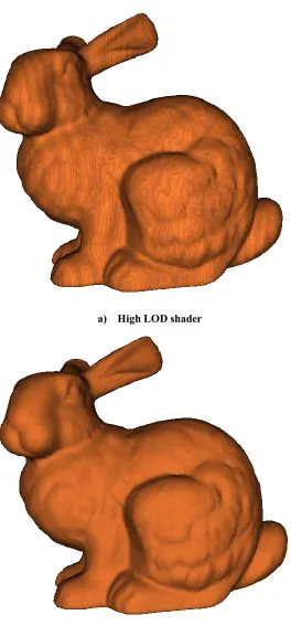
or when materials are very complex. Shader simplification involves the creation of multiple
shaders each with a different level of complexity. Shader simplification is an improvement
to the pixel manipulation portion of the graphics pipeline. Figure 7 shows the wood shader
defined in Figure 5 and Figure 6 applied to the Stanford Bunny at two levels of detail.
A significant problem associated with shader simplification is that it is a non-trivial
task to create multiple shaders that are simplified from an original in a logical and continuous
manner. Pellacini suggested a method of automatic shader generation in which the lines of
code in a shader are programmatically simplified based on a series of rules (Pellacini, 2005).
In order to create a smooth transition in areas where there would be a switch between two
shader levels of detail, it would be possible to blend two neighboring shaders together. Care
needs to be taken however, because it can be computationally expensive to switch between
a) High LOD shader
[image:25.612.190.454.95.671.2]b) Low LOD shader
The third target of simplification targets physics calculations. The complex physics
calculations required to create realistic interactions among irregularly shaped models can also
be a cause for reduced interactivity. Simulation simplification is not a method for alleviating
a bottleneck on the graphics card, but instead reduces the complexity of calculations
performed by the CPU before the data is transferred to the graphics card. It is a
simplification of the modeling portion of the rendering pipeline.
The physical representations of objects can be simplified to reduce the complexity of
physics calculations (O'Sullivan C. , Dingliana, Giang, & Kaiser, 2003). The highest level of
detail representation is the mesh itself. At the next lowest level of detail, the geometric
volume is filled using very small boxes where the boxes almost entirely occupy the same
amount of space as the geometric representation. As the level of detail decreases, the sizes of
the boxes used to fill the volume increase until at the very lowest level of detail, a single box
is used. The simulation representation for the interacting objects can also be approximated
using other primitive geometric objects whose motion is simple to calculate.
Another method of reducing the computation for physical simulations involves the
use of an interruptible algorithm (O'Sullivan, Radach, & Collins, 1999). The application is
allotted a certain amount of time in which to perform all of the collision detection
calculations in each frame. Once the time cut-off is reached, the objects in the scene are
placed in the positions and the orientations which had been computed. If the application had
not yet completed a calculation for a specific object, then the transform would not be as
accurate as those for which the calculations had been completed. This allows for improved
a) High Level of Detail Physical Representation
b) Low Level of Detail Physical Representation
Because the geometric representation and the simulation representations are separate
and distinct, one does not need to change both the geometric representation and the
simulation representation at the same time. Instead, they can be optimized individually.
Figure 8 shows two different ways a single object can be represented for physical simulation.
In the top image, the bunny is represented accurately by a mesh. In the bottom image, the
bunny is represented by a cube that is a simple bounding box. If all objects are simulated as
boxes, interaction between objects in a scene would be much easier to calculate. In both
images, the red lines indicate the representation for physical simulation. A medium level of
detail physical representation could be a further simplified mesh, or it could be a series of
cubes arranged to approximate the volume of the original model.
1.1.4. Representing Geometric Levels of Detail
There are three types of geometric level of detail (LOD) representations: discrete
level of detail, continuous level of detail, and view-dependent level of detail (Luebke, Reddy,
Cohen, Varshney, Watson, & Huebner, 2003). Choosing the appropriate representation
depends on many factors including the complexity of the original unsimplified environment,
the amount of memory that you have to store the representations, and the amount screen
space a single object will occupy. Table 1 describes the three different types of
representations.
Table 1. Common LOD Representations
Representation Stored As… Rendered as…
Discrete LOD Multiple files each of which
corresponds to a single LOD
A group of polygons based on a single most appropriate LOD.
Continuous LOD Single file loaded as a
hierarchy of separations and joins
A group of polygons based on a single most appropriate LOD.
View Dependent LOD Single file with separations and joins for specific areas of the model
Discrete level of detail representation is a method first used in flight simulators and is
used in most modern video games (Luebke, Reddy, Cohen, Varshney, Watson, & Huebner,
2003). In those systems, the level of detail decreases the farther away an object is located
from the observer. In the discrete level of detail representation, multiple versions of a single
model are stored. Figure 4 (page 10) shows the Stanford bunny at three discrete levels of
detail. Each version of the model corresponds to a level of detail which has been computed
and saved beforehand. Each version of the model must be loaded into memory at run time.
Because multiple versions of the same model must be kept in memory and the amount of
memory available is limited, the number of different versions needs to be restricted.
Otherwise, meshes for different levels of detail would have to be switched in and out of main
memory. Due to the limited number of levels which can be defined, “popping” can become a
big issue. Popping is a visual artifact that occurs during the switch between two different
levels of detail when the differences between two levels of detail are visually noticeable
(Luebke, Reddy, Cohen, Varshney, Watson, & Huebner, 2003). Popping is undesirable
because it is distracting and reduces the realistic feel of the environment.
A more complex level of detail representation is continuous level of detail. In a
continuous level of detail representation, an object is stored as a hierarchy of vertex splits and
merges. A schematic that demonstrates this concept is shown in Figure 9. In the schematic,
each circle in the tree represents a single vertex. At the bottom of the tree is the high-detail
representation with 4 vertices. In the low detail representation at the top of the tree, those 4
vertices have been joined to create a single vertex. Simplification is done by combining two
connected vertices into one vertex either through the elimination of one of the vertices or
through creating a new vertex which is an interpolation between the two vertices and
removing those two original vertices. It is only necessary to traverse the hierarchy until the
appropriate level of detail is reached. The geometric complexity of a model can be changed
between levels of detail because the difference in appearance between the two levels of detail
is small.
Sometimes there will be an object that is highly detailed and is located in the middle
of the field of view, taking up a large portion of the screen. With only continuous or discrete
level of detail representations, the entire object would need to be rendered at the highest level
of detail given that the user is looking at some part of this object. This would reduce the
degree of geometric simplification that would otherwise be possible. In this situation,
view-dependent level of detail representation is useful. In view-view-dependent level of detail
representation, a single large object which spans many levels of detail in the environment can
be rendered with a different level of detail for each portion of the display. When using
discrete or continuous level of detail representations, an environment can have multiple
levels of detail existing within the same frame, when using a view-dependent representation a
single model can have multiple levels of detail existing within the same frame. Figure 10
Figure 9. Continuous Level of Detail Representation
illustrates a terrain model with view-dependent level of detail representation. It was created
using ROAM (Duchaineau, 2003). The terrain in the image is stored as a single model, but
by using a view-dependent level of detail representation, the area in the lower right-hand
corner can be presented with more detail than the region in the upper left-hand corner.
1.2.
Visual Perception Background
Perceptually adaptive rendering research is also based on aspects of visual perception.
The first aspect is the physical anatomy of the eye and more specifically the retina. A second
aspect is how people go about collecting information when perceiving a scene. The third is
the role of attention in visual perception. Section 1.2 describes basic information about these
three aspects and their relation to perceptually adaptive rendering.
1.2.1. Anatomy of the Retina
The retina, lining the back of the eye, converts light into electrical signals in the
nervous system. A diagram of the eye is shown in Figure 11. Photoreceptors in the retina
are responsible for transducing the light received by the eye into electrical energy. There are
two types of photoreceptors: rods and cones. Rods are more numerous than cones and are
able to function under very low light levels. They are broadly sensitive across the light
spectrum. There are about 100 to 120 million rods on a single retina. Cones, on the other
hand, are less sensitive to light, but are responsible for our ability to sense color. Cones are
1/15th as abundant as rods, numbering between 7 and 8 million in a single retina. The
greatest concentration of cones is in a small area near the center of the retina called the fovea.
The fovea is only 1.5 mm in diameter (Ferwerda, 2001). If you hold your thumb at arms
length, the area of the real world that is projected onto the fovea in high resolution is
approximately the size of your thumbnail (Baudisch, DeCarlo, Duchowski, & Geisler, 2003).
The area of the visual field that projects to the fovea covers only 2 degrees of visual angle
(Cater, Chalmers, & Dalton, 2003). As a result of this non-uniform photoreceptor
arrangement, very little of the visual field is actually sensed at a high resolution.
Our ability to perceive detail decreases in relation to eccentricity, the angular distance,
from the fovea. As eccentricity increases, cone density decreases nearly exponentially. By
20 degrees eccentricity, the cone density asymptotes to a minimum. Rod density is higher in
the periphery than cone density. It decreases in the far periphery and approaches its minimum
density at 75 to 80 degrees (Ferwerda, 2001). This is why we perceive only the coarsest
information about objects located on the edges of our field of view.
1.2.2. Attention
Certain aspects of scenes are more likely than others to attract a person‟s attention.
Saliency is the measure of the likelihood for an object to attract one‟s attention. Properties of
a feature that make it more salient include brighter colors, movement, task importance,
location in the foreground, inclusion of patterns or faces, and familiarity to the user (Luebke,
Reddy, Cohen, Varshney, Watson, & Huebner, 2003). Although these characteristics are
known to attract attention, it is clear from the differing scan paths in Figure 12 that the
saliency value of a specific portion of a scene cannot be calculated merely from the inherent
properties of the scene or object alone.
Although it is possible to move attention without moving our eyes, it requires more
effort to move attention with fixed eyes (Rayner, 1998). Therefore, if an object captures our
attention, we are highly likely to move our eyes so that the object is viewed in detail using
the foveal region of the retina.
Change blindness and inattentional blindness are two behavioral phenomena related
to visual perception. Both are related to our inability to detect very significant changes in our
visual surroundings. Change blindness is the “inability of the human eye to detect what
should be obvious changes” (Cater, Chalmers, & Dalton, 2003). This phenomenon can occur
when the visual field is briefly disrupted. A participant is presented with a scene. The scene
been changed. The change is often undetectable because the participant cannot compare all
regions in the original and changed images (Simons, Nevarez, & Boot, 2005).
The body of change blindness research indicates that our internal representation of the
external world is much less detailed than our experience of “seeing” suggests (Cater,
Chalmers, & Dalton, 2003). We feel that were are able to see the entire world in complete
detail, but were are really only perceiving small portions of our environment and filling in the
holes with what our experience tells us should be there. Many studies of change blindness
use some sort of occlusion technique: either fully covering the image, or “splashing” blocks
of pixels over various parts of the image (Intille, 2002). It is also possible to mask changes
by making the transition very slowly (O'Regan, Rensink, & Clark, 1999). Eye blinks are
easily detectable and saccades can be determined using eye tracking, which make them good
targets for exploitation. Changes to objects in the environment could be timed to occur only
during a blink or a saccade. Changes to the most salient objects will tend to be detected
faster (Intille, 2002).
1.2.3. Scene Perception
In everyday life, we do not notice the decrease in visual acuity in the peripheral visual
field. This is because of the way we move our eyes when viewing a scene. We are
constantly making quick eye movements called saccades in order to get new information
about our environment. Our eyes are relatively still between saccades for about 200-300
milliseconds. That period of relative stillness is known as a fixation (Rayner, 1998). Our
eyes make saccades about three times per second (Henderson, 2003).
The path the eyes take while viewing a scene is not the same for everyone. It can
depend upon the task. Figure 12 shows the results of an experiment which tracked eye
movements while participants viewed Repin‟s „An Unexpected Visitor‟ (Yarbus, 1967).
paths have been superimposed on the original image. The scan paths may have been aligned
approximately.
At the top of Figure 12 is the unchanged picture. Figure 12b shows the scan path
which resulted when the participant viewed the scene freely. The scan path in Figure 12c is
from when the participant was asked to determine what everyone had been doing just before
the visitor arrived. When asked to remember the positions of objects and people the scan
path in Figure 12d emerged. In Figure 12e, the participant was asked to determine the ages of
all of the people in the scene. Figure 12f was the scan path when the participant was asked to
remember what everyone in the scene was wearing. The scan path in Figure 12g emerged
when the participant was asked to judge how long the visitor had been away. The
task-dependent nature of these scan paths means that it is very difficult to determine what region
of a scene is the focus of attention and thus displayed in high resolution based solely on
a) Original Image
b) Free examination c) What had the family been doing?
d) Positions of objects and people e) Give the ages of the people
f) What are the people wearing? g) How long had the visitor been away? Figure 12. Differing Scan Paths by Task
1.3.
Level of Detail Selection Techniques
Two techniques can be used separately or combined to select an appropriate level of
detail, reactive level of detail selection and predictive level of detail selection. Reactive level
of detail selection uses information that is provided while the application is running to
determine the appropriate level. Predictive level of detail selection uses the properties of the
object and scene to determine when to render a specific level of detail before the application
is run.
While the studies reviewed in this section are organized by their method of level of
detail selection, they vary on other characteristics as well. These include the method of
tracking, representation, basis for reduction and display type. Either head or eye tracking is
used to determine where the user is looking. The studies presented use discrete, continuous
or view-dependent representations. The method of reduction is either screen-based or
model-based.
Screen-based level of detail reduction seeks to reduce the bottleneck in the
rasterization portion of the graphics pipeline. This type of technique is most useful for
teleconferencing, where the original source is a 2D image. Model-based level of detail
reduction is for 3D content and involves reducing the geometric complexity of the models in
the scene to reduce the bottleneck in the vertex manipulation portion of the graphics pipeline.
These selection techniques have been demonstrated on monitors, head-mounted displays
(HMDs), and CAVEs.
1.3.1. Reactive Level of Detail Selection
Reactive level of detail selection has been employed most frequently. Reactive level
of detail selection methods utilize a direction of view or point of gaze in order to select the
appropriate level of detail. This is because when we are attending to things, we look at them.
simulators which used distance from the viewer within the view frustum to determine the
level of detail. Figure 13 shows a diagram of a top-down view of the scene illustrating the
regions of a scene that would be rendered at various levels of detail using this technique.
Distance-based reactive level of detail selection relies upon the fact that objects that
are farther away are rendered smaller on the screen. All that is needed to calculate the level
of detail is the distance between the user and the object. This works well for head-mounted
displays, because the field of view is relatively small. Figure 14 shows an implementation of
distance-based level of detail selection. In this figure, the bunny closest to the viewer is
rendered with the highest detail. The middle bunny is rendered at a medium level of detail.
The furthest bunny in the scene is rendered at the lowest level of detail. In the image on the
top, the distances have been compressed to show the three levels of detail. The image on the
bottom shows actual distances to illustrate the difficulty in distinguishing between the
appearances of the three levels of detail.
= user viewport (view frustum)
Figure 13. Top-Down Schematic Representation of Distance-Based LOD Selection
Low
Medium
a) Compressed distances
b) Actual distances
In eccentricity-based level of detail selection, objects in a direction away from the
direction of the gaze will be rendered in the lowest detail. The level of detail is determined
by an object‟s angular distance from the point of gaze. Figure 15 shows a diagram
illustrating the regions of a scene which would be rendered at each level of detail using
eccentricity-based level of detail selection using a top-down view of the scene.
Note: Gaze direction is from the center to the left
Figure 15. Top-Down Schematic Representation of Eccentricity-Based LOD Selection
Low
Medium High
An implementation of eccentricity-based level of detail selection is shown in Figure
16. In the top image, the user‟s gaze is aimed directly at the bunny. It is therefore rendered
in high detail. In the bottom image, the user‟s gaze is aimed slightly away from the bunny,
causing the model to be rendered at a lower level of detail. In order to determine the
appropriate level of detail for eccentricity level of detail selection, the point of gaze must be
determined either using head tracking or eye tracking. Because head movements closely
follow eye movements, head tracking can be sufficient for determining the center of gaze.
This is an easier method to apply given the high cost and awkwardness of eye trackers. The
disadvantage of using head tracking over eye tracking is that you will have to preserve a
larger region of high detail because you will be uncertain of the exact point of gaze (Watson,
Walker, & Hodges, 1997). With eye tracking, the user‟s point of gaze is pinpointed exactly,
and the degradation of rendered detail can correlate precisely with the reduction of visual
a) Looking at the object
b) Looking away from the object
Loschky and McConkie (1999) created an eccentricity-based system that used eye
tracking and a monitor for display. Their reduction method was screen-based involving a
high resolution area and a low resolution area. They set out to determine the earliest time
after an eye movement at which a change in the display could be detected. Visual sensitivity
is known to be greatly reduced during eye movements in order to suppress image blur caused
by the movement. They used monochromatic photographic scenes and discovered that any
change to the image must be made within 12 ms of the end of the eye movement. In their
study, their display took 7 ms to change an image, therefore the image change needed to be
initiated within 5 ms of the end of an eye movement. Saccade lengths were much shorter
when the high resolution portion of the image was only 2 degrees. This is important because
when saccades are shorter, more eye movements must be made to perceive the entire scene.
It was also found that perceivable changes such as delays of 15 ms or more severe
degradation did not have a large impact on task performance (Loschky & McConkie, 1999).
A later study showed that update delays of 45 ms do not impact the time required to find an
object, but do affect fixation durations (Loschky & McConkie, 2000).
Geisler, Perry and Najemnik (2006) used eye tracking to find gaze location in their
study. Their screen-based method involved 6-7 discrete levels displayed on a monitor. They
provided a 2D map which defined the appropriate resolution for every portion of a video
image based upon its eccentricity and direction from gaze. Blur was undetectable when the
region of reduction was 6 degrees.
Reingold and Loschky (2002) tested to see if creating a smooth boundary between the
two levels of detail impacted performance. Their reduction method was also screen-based
and was displayed on a monitor. They observed no significant difference between
performance when there was a smooth boundary between the two levels of detail and
Murphy and Duchowski (2001) created a virtual environment with a single
multi-resolution object. They were trying to determine the optimal view-dependent level of detail
for that object. Participants used a head mounted display and their eyes were tracked. The
model was originally rendered at a perceivably low level of detail. The level of detail was
gradually increased for different sections of the model, until the participant was no longer
able to perceive any change in detail. After finding the “optimal” level of detail based on
perception, frame rates were compared to discover the performance improvement of using
gaze-contingent rendering. When rendering 24 meshes of the Igea model in the same scene,
the best performance improvement was observed. If all 24 meshes were rendered at full
detail, frame rates were too slow to measure. Employing gaze-contingency improved frame
rates to 20 to 30 frames per second.
Watson, Walker, Hodges, and Worden (1997) used a HMD with a fixed inset relative
to the display screen creating two discrete levels of detail. In order to bring an object into
focus, the user moved his head. The paradigm is like “looking through a fogged glass mask
that has been wiped clean in its center” (Watson, Walker, Hodges, & Worden, 1997). Inset
displays performed better than displays of uniformly low resolution and did not perform
significantly worse than uniformly high resolution displays (Watson, Walker, & Hodges,
1995). The successful substitution of head tracking for eye tracking indicates that eye
tracking is not necessary when the inset is not extremely small. A later study showed that
using head tracking with a 45 degree inset can replace eye tracking (Watson, Walker, &
Hodges, 1997). Even though eye movements can be made outside of the 45 degree window,
if a new fixation point is selected more than 15 degrees away from the original starting point,
1.3.2. Predictive Level of Detail Selection
While reactive level of detail selection methods directly find the center of gaze,
predictive level of detail selection methods seek to determine ahead of time what will attract
our focus. Since what attracts our attention is most likely to also be the focus of our gaze, the
level of detail can be selected based on how likely it is for each object in the environment to
attract attention.
Minakawa, Moriya, Yamasaki, and Takeda (2001) created a system using a motion
ride—a chair with hydraulics which gives the user a sense of motion—in a CAVE. The
motion ride limited the user‟s movements and served as a proxy for a head tracker. Because
the position in the environment was always known, the experimenters were able to pre-render
all of the images. The images presented in this experiment were from a 2D source, and thus
a screen-based reduction method was used. Extra detail was provided on the front screen of
the CAVE with two extra projectors. The ride apparatus limited the user‟s range of motion;
therefore the front wall was the most likely target for attention. The system employed two
discrete levels of detail. A section in the middle of front wall was rendered with a high
resolution and the rest of the walls were rendered at a uniformly lower resolution. No
information about perceptual benefits was provided.
Certain features make an object more likely to be the focus of attention. These
features include brighter colors, movement, task importance, location in the foreground,
inclusion of patterns or faces, and familiarity to the user (Luebke, Reddy, Cohen, Varshney,
Watson, & Huebner, 2003). By calculating the influence of these features you can create a
saliency map of the most important objects in the environment. A saliency map represents
the visual importance of each portion of the visual field topographically. The color of a
region indicates how important that region is and how likely it will be to attract attention.
For predictive level of detail selection, the objects with the most saliency should be rendered
Another feature that can be used to predictively select the appropriate level of detail is
motion. While motion does attract attention, we also do not have as much time to focus on
the details of objects that are quickly moving across the screen. This means that we can
render fast-moving objects at a lower level of detail than slower-moving or still objects in the
same environment.
Parkhurst and Niebur (2004) employed a velocity-based predictive level of detail
selection technique. A model-based reduction technique was used and the display was a
monitor. The models used a continuous level of detail representation. All objects in the
scene were stationary, so the velocity was based upon the motion created by the rotation of
the viewport. The rotation of the viewport caused a reduction in the level of detail of objects
in the scene. As the rotation slowed, the level of detail of the objects increased. The time it
took to search for objects in the scene was not affected by the level of detail reduction, but
the highly variable frame rates did make it more difficult to localize the target objects.
1.3.3. Summary
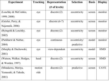
Table 2 provides a breakdown of the key differences in the experiments described in
this section 1.3. Most of the described experiments employed eye tracking and screen-based
reduction of 2D images. Discrete representations of the levels of detail were created
selection the appropriate level of detail was eccentricity-based. Most of these rendering
Parkhurst and Niebur (2002) provided some considerations for evaluating the
feasibility of a variable resolution display. A conservative estimate of the visual field is 180
horizontal degrees by 100 vertical degrees. Adaptive rendering has the potential to improve
rendering performance more when using a head mounted display than on a computer monitor
because it has approximately double the field of view. Actual improvements on rendering
performance are also a function of eye (or head) tracker sampling rates, software drawing
routing, and display refresh rate.
1.4.
Immersive Virtual Reality Environments
Head mounted displays and CAVEs present a larger field of view than desktop displays.
[image:47.612.93.543.120.455.2]The limited field of view of a desktop display can cause the user to collide with walls and
Table 2. Summary of Relevant LOD Research
Experiment Tracking Representation
(# of levels)
Selection Basis Display
(Loschky & McConkie, 1999; 2000)
eye discrete (2) eccentricity screen monitor
(Geisler, Perry, & Najemnik, 2006)
eye discrete (6-7) eccentricity screen monitor
(Reingold & Loschky, 2002)
eye discrete (2) eccentricity screen monitor
(Parkhurst & Niebur, 2004)
eye continuous eccentricity/
predictive
model monitor
(Murphy & Duchowski, 2001)
eye view-dependent eccentricity model HMD
(Watson, Walker, Hodges, & Worden, 1997)
head discrete (2) eccentricity screen HMD
(Minakawa, Moriya, Yamasaki, & Takeda, 2001)
motion ride
doorways in virtual environments (Duh, Lin, Kenyon, Parker, & Furness, 2002). This is
because it interferes with the creation of a spatial map of scene and thus make navigation
more difficult. Immersive virtual reality systems are able to provide the user with an
environment more consistent with reality and therefore do not hinder navigation as much.
Displays with a limited field of view also limit the number of items that can be
simultaneously displayed (Tory & Möller, 2004). If more items are included, all of the items
must be displayed in less detail in order to fit in the visual scene space. On the other hand,
reducing the number of items makes it harder to see the relationship between all of the items.
The user must either keep more detail or context information in working memory. The extra
cognitive load could adversely affect performance. Displays which provide a larger field of
view alleviate the demand for visual scene space, but creating large immersive displays also
requires rendering more vertices and pixels.
The method of displaying a virtual environment greatly impacts how a user can
interact with the environment. Because so little of the visual input that we perceive is in high
resolution, we can work to render each piece of the environment at the lowest level of detail
that is perceptually indistinguishable from its non-degraded counterpart. For fully immersive
environments, an eccentricity-based level of detail selection is better because it takes into
consideration our limited horizontal field of view. In an immersive environment, if the level
of detail were selected simply based on distance, much of the scene would needlessly be
rendered in high detail. Using distance-based level of detail selection, an object located
behind the user would be rendered in high detail because the distance from user to object is
small. By employing eccentricity-based level of detail selection instead, that object would be
1.5.
Research Approach
The purpose of this research was to determine if perceptually adaptive rendering
techniques can improve the quality in an immersive virtual environment. Perceptually
adaptive rendering has the potential to improve frame rates while maintaining the detail
needed by the user to perform tasks in virtual reality. The increased interactivity provided by
faster frame rates will hopefully counterbalance the reduced peripheral detail to improve the
user‟s overall experience of immersive virtual reality.
The first component of this research was the design of a new perceptually adaptive
rendering system which is capable of running on immersive virtual reality hardware. The
rendering system supports rapid authoring of virtual environments. This allows for the
construction and storage of multiple unique environments. These environments can be
displayed without recompiling the source code. Level of detail can be determined using an
eccentricity-based technique. The eccentricity-based technique can be combined with an
attentional hysteresis factor to prevent objects located at the first threshold angle from
switching back and forth repeatedly. Attentional hysteresis is explained further in section
2.2.2.
The second component of this research is the evaluation of the perceptually adaptive
rendering system. In order for the system to be useful, it must increase interactivity by
providing higher frame rates than if the environment were rendered in uniformly high detail.
Also, the changing level of detail must not create extra distraction for the user. In order to
validate the system based on these qualifications, a full study and a pilot study were
performed.
The experimental approach in this thesis is motivated by prior research on
perceptually adaptive displays (Parkhurst & Niebur, 2004). This study used a realistic living
room environment, shown in Figure 17. The environment was rendered on a desktop
level of detail. The appropriate level of detail was determined based on eccentricity, with an
eye tracker determining the participant‟s gaze location. An object was considered found
when the user moved a crosshair over the correct target object. Although it took longer to
localize target objects, none of the participants reported anything unusual about the
environment even when prompted.
Parkhurst and Niebur showed that perceptually adaptive rendering could be beneficial
even in the limited screen space of a desktop monitor. The research in this thesis focuses on
using similar techniques in an immersive environment where the potential benefits are even
greater. Discrete levels of detail will be used because no existing virtual reality software