HarpLDA+: Optimizing Latent Dirichlet Allocation for Parallel Efficiency
Bo Peng1 Bingjing Zhang1 Langshi Chen1 Mihai Avram1 Robert Henschel2 Craig Stewart2 Shaojuan Zhu3 Emily Mccallum3 Lisa Smith3 Tom Zahniser3 Jon Omer3 Judy Qiu1
1School of Informatics and Computing, Indiana University 2UITS, Indiana University
3Intel Corporation
{pengb, zhangbj, lc37, mavram, xqiu}@indiana.edu {henschel, stewart}@iu.edu
{shaojuan.zhu, emily.l.mccallum, lisa.m.smith, tom.zahniser, jon.omer}@intel.com
Abstract—Latent Dirichlet Allocation (LDA) is a widely used machine learning technique in topic modeling and data analysis. Training large LDA models on big datasets involves dynamic and irregular computation patterns and is a major challenge to both algorithm optimization and system design. In this paper, we present a comprehensive benchmarking of our novel synchronized LDA training system HarpLDA+ based on Hadoop and Java. It demonstrates impressive performance when compared to three other MPI/C++ based state-of-the-art systems, which are LightLDA, F+NomadLDA, and WarpLDA. HarpLDA+ uses optimized collective communication with a timer control for load balance, leading to stable scalability in both shared-memory and distributed systems. We demonstrate in the experiments that HarpLDA+ is effective in reducing synchronization and communication overhead and outperforms the other three LDA training systems.
I. INTRODUCTION
Latent Dirichlet Allocation (LDA) [1] is a widely used machine learning technique in topic modeling and data analysis. LDA training is an iterative process, which starts from a randomly initialized model with parameters to learn, iteratively computing and updating the model until it con-verges. A major challenge of scaling is due to the fact that computation is irregular and the model size can be huge. In the meantime, parallel workers need to synchronize the model continually.
State-of-the-art LDA training systems (trainers) are imple-mented to handle billions of documents, hundreds of billion tokens, millions of topics and millions of unique tokens. However, the pros and cons of different approaches in the existing tools are often hard to explain because of the many trade-offs between effectiveness (contributions to converge) and efficiency (computational cost) of model updates. Note that model update efficiency should be distinguished from the traditional parallel efficiency of speedup over paral-lelism.
One of the popular approaches is to decrease the time complexity of the computation by introducing approxima-tions. Another widely used idea is to reduce the synchro-nization overhead by using an asynchronous parallel system working on a stale model, where the trainer is not using
the latest model data. Although these approaches improve model update efficiency, they are done at the cost of the model update effectiveness for convergence. Our approach however, is to use a synchronized system and optimize LDA trainers from a different perspective. The aim is to preserve the effectiveness and at the same time improve parallel efficiency by reducing the synchronization overhead.
Our main contributions can be summarized as follows:
• Review state-of-the-art LDA training systems and sum-marize their design features.
• Propose new mechanisms to reduce overhead in syn-chronized systems, dynamic scheduling for shared memory subsystems and Timer Control for distributed systems.
• Implement HarpLDA+ based on Hadoop while
demon-strating excellent performance and scalability.
• Summarize our system design approach and its impli-cations for other machine learning algorithms. In this paper, Section II introduces the background of the LDA algorithm and related work, while Section III analyzes the architecture and parallel efficiency of existing solutions. Section IV describes our system design and implementation details of HarpLDA+ and Section V presents experimental results coupled with a performance analysis. Finally, Sec-tion VI draws conclusions and discusses future work.
II. LDA ALGORITHM ANDRELATEDWORK
A. LDA with Collapsed Gibbs Sampling
xij=w zij=k
Nwk Mkj
Observed DATA MODEL to Learn
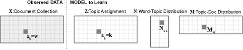
[image:1.612.316.557.592.642.2]X:Document Collection Z:Topic Assignment N:Word-Topic DistributionM:Topic-Doc Distribution
Figure 1: Latent Dirichlet Allocation.N and M are suf-ficient statistics for the probability distribution φ and θ respectively in the original graphical model.
as a collection of documents, where each document is a bag of words. LDA models each document as a mixture of latent topics and each topic as a multinomial distribution over words.
Many algorithms have been proposed to estimate the parameters for the LDA model. Collapsed Gibbs Sampling (CGS) [2], a Markov chain Monte Carlo (MCMC) algorithm, is commonly used for large scale LDA training. In the MCMC framework, samples can be drawn according to the unknown posterior distribution by a carefully designed transition function that visits the whole parameter space. Gibbs sampling is one such design that visits the parameter space from one dimension to the other. For each iteration, it fixes all the states of other dimensions and only updates the current visiting one.
In CGS, each training data point or token is assigned to a random topic denoted aszij at initialization. Then it begins
to reassign topics to each token at positioniin documentj, xij =w, by sampling from a multinomial distribution of a
conditional probability ofzij as shown below:
p zij =k|z¬ij, x, α, β∝
Nwk¬ij+β
P
wN
¬ij
wk +V β
Mkj¬ij+α
(1) Here superscript¬ij indicates that the corresponding token is excluded. V is the vocabulary size, Nwk is the token
count of word w assigned to topic k in K topics, and Mkj is the token count of topic k assigned in document
j. The matrices Z, N and M, form the model to be learned. Hyper-parametersαandβ control the topic density in the final model. The model gradually converges during the process of iterative sampling.
Although CGS generally requires a large number of iterations to converge, it is memory efficient and therefore scalable for large models. In this paper, we focus on the LDA trainers under the CGS algorithm family.
B. Related Work on Parallel LDA-CGS
Gibbs sampling in LDA-CGS is a strictly sequential pro-cess. Approximate Distributed LDA (AD-LDA)[3] proposed to relax the requirement of sequential sampling of topic assignments based on the observation that the dependence between the update of one topic assignment zij and the
update of any other topic assignmentzi0j0 is weak. In AD-LDA, the distributed approach is to partition the training data for different workers, run local CGS training and
synchronize the model by merging back to a single and
consistent set of N. PLDA [4] implemented the AD-LDA algorithm in both MPI and MapReduce, where the Allreduce operation was used for synchronization.
A synchronized algorithm that requires global
synchro-nization at each iteration sometimes may not seem feasible or efficient; Therefore, an asynchronous solution becomes the alternative choice. Async-LDA [5] extended AD-LDA to
an asynchronous solution by a gossip protocol. YahooLDA [6][7] was the first production level LDA trainer. The mechanism is an asynchronous reconciliation of the model, one word at a time for all samplers. Furthermore, Parameter Server [8] was introduced as a general framework that scaled to thousands of nodes. Another advancement was presented by [9]. It proposed a “mixed” approach SSP (Stale Synchronous Parallel), which is a parameter server that can limit the maximum age of the staleness.
Some researchers have investigated synchronized algo-rithms. For instance, a novel data partitioning scheme [10] was proposed to avoid memory access conflicts on GPUs. The basic idea is to partition the training data into blocks, where all samplers start from the diagonal blocks and then shift to the right neighbor all together. In contrast, a general machine learning framework Petuum Strads [11][12] extended this idea, where parameters of the ML program were partitioned for different workers. As this type of com-munication pattern observed in the asynchronous trainers is hard to optimize, synchronized designs were proposed with collective communication operators [13] which achieved bet-ter performance. Finally, F+NomadLDA [14] was introduced based on the idea of NOMAD [15], in which each variable (one row ofN) becomes the basic unit to be scheduled, and the ownership of a variable is asynchronously transferred between workers in a decentralized fashion.
Other research involves optimization to the sampling al-gorithm. According to Equation (1), a naive implementation involves drawing a sample from a discrete distribution which contains two steps: first calculate the probability of each event as p(zij = k), k ∈ K, secondly generate a random
number uniformly from[0−1)and search linearly along the array of the probabilities, stopping when the accumulation of probability mass is greater than or equal to the random number. The time complexity for this isO(K). SparseLDA [16] decomposed the numerator of Equation (1) into three parts: αβ, β ∗Mkj¬ij and Nwk¬ij(Mkj¬ij +α). The first part is a constant; while the second part is non-zero only when Mkj is non-zero, and the third part is non-zero only when
Nwkis non-zero. Both the probability calculation and search
part can benefit from utilizing the characteristics of this sparseness pertaining to the model. When using this feature, the computation time complexity drops to O(Kd +Kw),
which is equivalent to the average number of non-zero items in column of M and row of N and is typically much smaller than K. F+NomadLDA provides an optimization on the search part by using a O(logK) binary tree search instead of a O(K) linear search by a tree data structure. Based on Alias Table which allows us to draw subsequent samples from the same distribution inO(1)time, Alias-LDA [17] uses the Metropolis Hasting (MH) sampling process to draw each sample correctly from the stale alias table and achieves O(Kd) complexity. LightLDA [18] extends
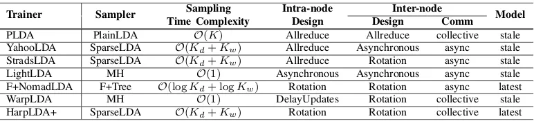
Trainer Sampler Sampling Intra-node Inter-node Model
Time Complexity Design Design Comm
PLDA PlainLDA O(K) Allreduce Allreduce collective stale YahooLDA SparseLDA O(Kd+Kw) Allreduce Asynchronous async stale StradsLDA SparseLDA O(Kd+Kw) Allreduce Rotation async stale
LightLDA MH O(1) Asynchronous Asynchronous async stale
F+NomadLDA F+Tree O(logKd+ logKw) Rotation Rotation async latest
WarpLDA MH O(1) DelayUpdates Rotation collective stale
[image:3.612.114.500.70.158.2]HarpLDA+ SparseLDA O(Kd+Kw) Rotation Rotation collective latest
Table I: System Architectures of LDA Trainers. AllReduce, works on a stale model and does synchronization on model replicas.Asynchronous, works on local replicas and synchronizes them in a best effort through a group of parameter servers.
Rotation, works on distributed model partitions and the model partitions ‘rotate’ among the workers while at the same time
keeping model updates conflict free.
parts and alternating the proposals into a cycle proposal, thus achievingO(1)complexity. WarpLDA [19] introduces a more aggressive approach based on the idea of MH to delay all the updates after sampling one pass ofZ, by drawing the proposals for all tokens before computing any acceptance rates.
HarpLDA+, however, adopts the standard SparseLDA sampling algorithm and a synchronized system design in order to preserve the effectiveness of the model update while improving the parallel efficiency.
III. PARALLELDESIGNPRINCIPLES
A. Parallel Efficiency
Parallelizing a sequential algorithm inevitably introduces overhead. Parallel efficiency can be measured by Speedup, which is defined as parallel performance over original se-quential performance in parallel processing, where we have:
Speedup= T1
TP
= 1
f+s+1−Pf (2)
With P workers, f is the serial portion that cannot be parallelized and parallelism introduces a time overhead of sxT1. In parallel CGS,f is small, so the overhead time of sbecomes the major issue in order to achieve good parallel efficiency. Communication overhead comes from the addi-tional cost of moving data among the parallel workers. In a shared memory system, this overhead is generally ignored with the assumption of a uniform memory access cost. In a distributed system, asynchronous communication or pipelin-ing can be used to overlap communication with computation and reduce this overhead.Synchronization overhead comes from the additional cost of coordinating parallel workers that reach the same state in order to finish a task together. Asynchronous trainers try to reduce this type of overhead by avoiding a global consensus, relaxing the consistency of the model and working in an independent fashion. Synchronized trainers, however, will face the issue of load imbalance, which is a major source of synchronization overhead.
Some data partitioning algorithms have been proposed that aim to improve load balancing for LDA training. For
example, random permutations on the document usually give good results. Some algorithms partition the word-topic model, whereas randomized algorithms do not perform as well as greedy algorithms [13][19] since the word frequency follows the power-law distribution. Unfortunately, even op-timal partitioning algorithms cannot completely solve the load imbalance problem. Sampling algorithms may perform differently on the same number of tokens with different distributions. In practice, variations of node performance and stragglers are not uncommon even in homogeneous HPC clusters.
B. System Architectures
Machine learning algorithms can generally tolerate some kind of staleness in the model. Using stale models in computation can degrade the convergence rate but potentially boost the system efficiency because it relaxes the constraints for system design. For example, the sum of the topic count
P
wNwk in the denominator of Equation (1) is hard to keep
in strict consistency while in a parallel situation, because using locks on data being frequently accessed will give poor performance. A typical solution is to remove the locks and keep using a local copy of the model. Furthermore, synchro-nizing the model at the end of each epoch is sufficient as the deviations are small. However, the decision of whether to use stale values of Nwk and Mkj in the numerator of
Equation (1) is more sensitive to model convergence. In order to better present HarpLDA+’s design, we sum-marize the features and parallel architectures of current CGS trainers in a model centric view (see Table I).
IV. HARPLDA+: DESIGN ANDIMPLEMENTATION HarpLDA+ builds upon Harp1, which includes a Java collective communication library released as a plugin for Hadoop. While our previous work [13] optimizes commu-nications in different architectures, HarpLDA+ focuses on the Rotation architecture and reducing the synchronization overhead.
A. Programming Model Based on Collective Communica-tion
Collective communication within a Rotation design is easy to program. For each iteration, all workers concurrently sample on a local training data partition with a local model split without conflicts in model updates. Afterwards, a call to a collective communication operator ‘rotate’ is made, in order to exchange the model partitions globally. (see Algorithm 1)
Algorithm 1: HarpLDA+ Parallel Pseudo Code
input :training dataX,P workers, modelA0, number of
iterationsT
output:AT
1 parallel forworker p∈[1, P]do
2 fort= 1 to T do
// initialize: model At0 is At−1
3 fori= 1 toP do
// update local model split by sampling on local training data
4 Atpi0 =Sampling(Xp, A ti−1
p0 )
// synchronization to exchange model splits
5 rotate(Atpi0)
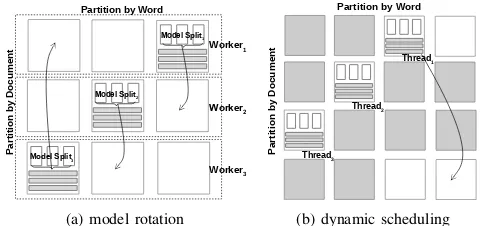
A concrete scheduling strategy is built into the ‘rotate’ operator. So long as each model split is owned by only one worker, the scheduling strategy guarantees to be conflict free. For instance, when a rotate call returns, all the workers can continue sampling concurrently without causing conflicts when updating the model. A default strategy shifts the model splits to their neighbor nodes (see Fig. 2a). Selecting the neighbor on a random permutation of the node list is also easy to implement. Furthermore, a priority based scheduler and a work load based scheduler can be implemented in this framework without losing the simplicity of the programming model.
Algorithm 1 presents a general framework for scheduling, where multi-threading and distributed parallelism can adopt the same procedure. We can however improve it to reduce synchronization overhead, leveraging the computation char-acteristics in these two different environments.
B. Dynamic Scheduling in Shared Memory systems
Dynamic scheduling provides a low cost solution to remove synchronization overhead in the shared memory system. It dynamically assigns workload to idle threads in order to increase the throughput of tasks. This is an effective solution, which is also used in parallel matrix factorization for recommender systems [20].
Partition by Word
Worker2
Worker3
Model Split1
P
ar
ti
ti
o
n
b
y
D
o
cu
m
en
t Worker1
Model Split
2
Model Split3
(a) model rotation
Partition by Word
P
ar
ti
ti
o
n
b
y
D
o
cu
m
en
t
Thread2
Thread3
Thread1
[image:4.612.319.559.82.195.2](b) dynamic scheduling
Figure 2: Model Rotation Framework and Dynamic schedul-ing in Shared Memory
In Fig. 2b, training data is partitioned into blocks, with the row partition using a random permutation of document id and the column partition using a greedy algorithm based on word frequency. Indexes are constructed during the initialization phase in order to build the map from word id to the related documents appearing in each block. In this case, the minimal unit for scheduling is a block. Furthermore, the number of partitions is larger than the number of threads, which means that there are always ‘free’ rows and columns when one thread finishes its current task. In this example,
thread 1 finishes first, then the scheduler selects a new
block randomly from the ‘free’ blocks, which are the white blocks in the figure. Becausethread 2andthread 3are still working, the rows and columns are occupied accordingly as denoted by the gray blocks. In a shared memory system, the scheduler does not move data but instead assigns data addresses of selected free blocks to the idle threads. The wait time of the threads are bounded by the overhead of the scheduler. In the case the number of threads is P and the number of splits isL, so aL×Lmatrix maintains a two level status: free, or finished. The scheduler can randomly select a free block by scanning the matrix with time complexity of no more than O(L2). The larger the L, the lower the number of conflicts and lower the wait time, but the more overhead introduced by the scheduler itself. Thus, there is a trade-off. By experimentation, we found thatL=√2P is a good choice in most cases.
C. Pipelining and Timer Control in Distributed Systems
inner loop of algorithm 1 is modified to become a loop over each slice. Consequently, the original rotate call becomes two rotate calls on each slice. As long as the communication time is less than the computing time spent on one slice, the pipeline will be effective in hiding the overhead from communication.
Another overhead of a rotate call is the time taken waiting for all workers to complete their computation. In the presence of load imbalance, all workers wait for the slowest one to finish. To solve this problem, we first discuss the sampling order of the Gibbs Sampling Algorithms. We note that LDA trainers can use two common scan orders: random scan and deterministic scan. For a Gibbs sampler, the usual deterministic-scan order proceeds by updating firstx1, then x2, thenx3, . . .xdand back tox1, visiting the state spaceX by a sequential order. Another random scan version usually proceeds at each iteration by choosing i uniformly from
1,2, ..., d. It has been demonstrated [21] that the sampling order affects the convergence rate of different models but a deterministic scan is commonly used to gain the benefits of hardware locality. This is the situation in current LDA trainers, in which sampling occurs over document or over word onZvia deterministic scan. Generally, the order with a better memory cache hit rate gives a better performance. For large datasets with V << D, word order is better. It is hard to achieve good performance with a pure random scan due to the cache miss issues. However, HarpLDA+ uses a quasi-random order. The dynamic scheduler picks a block uniformly from the free block list. While inside the block, we still keep the word sampling order. Although no significant performance difference is observed for the different sampling orders in LDA-CGS, we found that the random sampling order provides a natural solution for load balancing.
Worker1
rotate rotate
Time
Worker2
Worker3
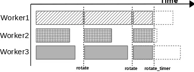
[image:5.612.77.269.498.569.2]rotate_timer
Figure 3: Timer to Control the Synchronization Point
For a given worker in Fig. 3 the white space between two rotate operations denotes the wait time between the end of the computation and the start of synchronization. If we adjust the synchronization point ahead before the computation finishes, the gap of wait time can be closed. Under the deterministic scan order, the adjustment is harder to achieve due to the housekeeping work needed and the original scan order is lost. For a random scan, this adjustment does not change the property of the uniform random selection of blocks. The third rotate call demonstrates this mechanism
in Fig. 3.
We further propose a simple solution for the LDA-CGS trainer. Each sampler only works for the same period of time and then the samplers do synchronization all together. They all use a timer to control the synchronization point rather than waiting until all the blocks to finish. Because the model size shrinks and the computation time drops during the process of convergence, we’ve designed an auto-tuning mechanism to set the value of the timer for each iteration in HarpLDA+.
First, the timer works best when the communication can be fully overlapped by computation, where the computation time or the number of training data points being processed should have a lower bound L. Secondly, we make sure that all workers stop at the same time before any of them complete their work. This implies an upper boundH.Land H are set as input parameters. In normal cases,L= 40%, H= 80% are good choices.
We set up heuristic rules to automatically determine the values of timerti based on theL, H settings.
• Rule 1: During the first iteration, we set the timer to
a constant t0, and obtain the processing ratio R0 for each worker at the end of the iteration.
• Rule 2: WhenRi is found to be smaller thanL, adjust
ti+1=ti∗2 in order to quickly catch up. (In the first
iteration, repeat this step untilRi+1 is in the range of LandH.)
• Rule 3: When Ri is found to be larger than H,ti+1 will be reduced in half.
D. Other Implementation Issues
For a high performance parallel LDA trainer, besides the key factor of the original sampling algorithm and the parallel system design, implementation details may also be important. HarpLDA+ is a Java application, where primitive data types are used in critical data structures. For instance, we found that using primitive arrays with array indexing for the model matrix is significantly faster than using a hashmap in HarpLDA+. Furthermore, minor improvements for SparseLDA are very helpful. Topic counts are sorted periodically to reduce the linear search time of sampling. Caching is also used to avoid repeat calculations. When sampling multiple tokens with the same word and document, the topic probabilities calculated for the first token are reused for the tokens that follow.
V. EXPERIMENTALEVALUATION
A. Setup of Experiments
Five datasets are used in the experiments (see Table II), which are open datasets in related work. Here, pubmed2m is a subset of Pubmed Dataset2, clueweb30b is a subset of
0 1000 2000 3000 4000 5000 6000 Training Time (s) 1.00 0.95 0.90 0.85 0.80 0.75 0.70 0.65 0.60 0.55 Model Log-likelihood
1e9 Convergence Speed
0 50 100 150 200 Epoch Number 1.00 0.95 0.90 0.85 0.80 0.75 0.70 0.65 0.60 0.55 Model Log-likelihood
1e9 Convergence Rate
0 1000 2000 3000 4000 5000 6000 Training Time (s) 105 106 107 108 Throughput (tokens/s) Throughput
0 100 200 300 400 500 Training Time (s) 1.00 0.95 0.90 0.85 0.80 0.75 0.70 0.65 0.60 0.55 Model Log-likelihood
1e9 Convergence Speed
1 2 4 8 16 32 64 Number of Threads 20 21 22 23 24 25 26 SpeedUp TP(N)/TP(1)
Speedup in Throughput
0 2000 4000 6000 8000 10000 Training Time (s) 1.4 1.2 1.0 0.8 0.6 Model Log-likelihood 1e9
0 50 100 150 200 Epoch Number 1.4 1.2 1.0 0.8 0.6 Model Log-likelihood 1e9
0 2000 4000 6000 8000 10000 Training Time (s) 105
106 107 108
Throughput (tokens/s)
0 500 1000 1500 2000 Training Time (s) 1.4 1.2 1.0 0.8 0.6 Model Log-likelihood 1e9
1 2 4 8 16 32 64 Number of Threads 20 21 22 23 24 25 26 SpeedUp TP(N)/TP(1)
0 20000 40000 60000 80000 100000 Training Time (s) 1.3 1.2 1.1 1.0 0.9 0.8 0.7 0.6 Model Log-likelihood 1e10
0 50 100 150 200 Epoch Number 1.3 1.2 1.1 1.0 0.9 0.8 0.7 0.6 Model Log-likelihood 1e10
0 20000 40000 60000 80000 100000 Training Time (s) 105
106 107 108
Throughput (tokens/s)
HarpLDA+ LightLDA F+NomadLDA WarpLDA
0 1000 2000 3000 4000 5000 6000 Training Time (s) 1.3 1.2 1.1 1.0 0.9 0.8 0.7 0.6 Model Log-likelihood 1e10
[image:6.612.62.553.71.302.2]1 2 4 8 16 32 64 Number of Threads 20 21 22 23 24 25 26 SpeedUp TP(N)/TP(1)
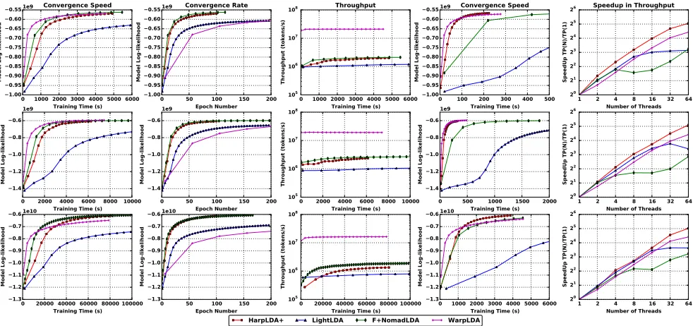
Figure 4: Single Node Performance with 3 rows corresponding to 3 datasets nytimes (K= 1000), pubmed2m (K= 1000), enwiki (K = 10000) respectively. The columns are different observables with columns 1 to 3 reporting sequential single thread measurements and column 4 with 32 threads. Column 5 plots the results against different thread counts. Each column corresponds to an evaluation metric denoted in the title.
Dataset Docs V ocabulary T okens DocLen
nytimes 299K 101K 99M 332/178
pubmed2m 2M 126K 149M 74/33
enwiki 3.7M 1M 1B 293/523
bigram 3.8M 20M 1.6B 434/767
[image:6.612.66.287.376.436.2]clueweb30b 76M 1M 29B 392/532
Table II: Datasets for LDA Training, whereDocLen repre-sents mean and std. dev. values of document length
ClueWeb09 Dataset3, enwiki is built from English articles from Wikipedia and bigram is a bigram version of enwiki dataset.
trainer language multithreading communication LightLDA C++ Pthread Zeromq+MPI
NomadLDA C++ Intel TBB MPI
WarpLDA C++ OpenMP MPI
HarpLDA+ Java Java Thread Harp Collective
Table III: Trainers for Experiments
We select four state-of-the-art CGS trainers for com-parison in Table III. They represent the different system designs described in Section III-B. Also different versions of HarpLDA+ are included, e.g., Harp-nods without dynamic scheduling, and Harp-notimer without timer control.
To evaluate the performance, we use the following met-rics. Firstly, we choose Model log likelihood of the
word-3http://lemurproject.org/clueweb09.php/
topic model to represent the status of convergence. Secondly, we select three main evaluation metrics as follows: 1)
Convergence rateevaluates the effectiveness of the algorithm
by depicting the relationship between convergence level and model update count. 2)Throughputevaluates the efficiency in a system view by measuring the model update counts per second. 3)Convergence speed is the metric to evaluate a trainer’s overall performance, which depicts the relation between convergence level and training time(initialization time excluded). It represents the overall performance result-ing from the combination of efficiency and effectiveness of model updates.
nodes andmthreads on each node and is denoted asn×m in the following diagrams. On a similar note, K signifies the number of topics used in the LDA trainers.
B. Experimental Results
1) Performance of Sequential Algorithm: We first analyze
the performance of the sampling algorithm by evaluating the trainers in a single thread setup.
As shown in Fig. 4, in column 1 ofConvergence Speed, WarpLDA is the fastest trainer due to its successful trade-off between the efficiency and effectiveness of updates. Furthermore, F+NomadLDA is faster than HarpLDA+ and demonstrates even better performance than WarpLDA in the case of large K. For this assessment, LightLDA is consistently the slowest.
Column 2 of Convergence Rate shows that F+NomadLDA, a standard SparseLDA sampler, always runs the fastest. HarpLDA+ is a bit slower due to the caching of the model for identical words. Both MH samplers, LightLDA and WarpLDA are significantly slower since they are an approximation for the original CGS, while WarpLDA is the slowest because of its update delay strategy making each update much less effective. The rank of convergence rate is consistent in parallel versions of these trainers.
In column 3 ofThroughput, WarpLDA shows much better throughput than the others due to optimization of memory use obtained from removing the random matrix access. Among the others, F+NomadLDA performs slightly better.
2) Intra-node Parallel Efficiency: We run a test by
in-creasing number of threads in order to evaluate its impact on performance. As seen in Fig. 4, column 4, the convergence speed at 32 threads shows that the performance rank of F+NomadLDA drops, and HarpLDA+ takes its place and runs as well as WarpLDA at K = 1000 and exceeds it’s performance forK= 10000. In Fig. 4 column 5 ofSpeedup
in Throughput, HarpLDA+ demonstrates the best parallel
efficiency which explains the boost of its performance from a single thread to a large number of threads.
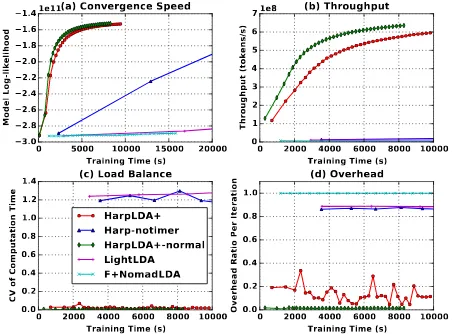
Concurrency Analysis by VTune Amplifier4 is utilized to exhibit the time breakdown with normalized results in Table IV. WarpLDA demonstrates excellent efficiency, as it not only decouples the memory access to the two model matrices but also removes the model update conflicts, in which all threads are running in a pleasingly parallel fashion programmed in OpenMP. In this implementation, load imbalance is observed to contribute to the 9% wait time. This may come from the default static scheduler in OpenMP. NomadLDA has zero wait time, but this does not necessarily signal efficiency. All threads keep trying to pop a model column from the concurrent queue to run sampling, and yield when the pop call fails. A large number of yield calls are observed to give 24% on spin time. Load
4https://software.intel.com/en-us/intel-vtune-amplifier-xe
Trainer CPU Time Wait
Effective Spin Overhead Time
WarpLDA 0.91 0 0 0.09
NomadLDA 0.75 0.24 0 0
LightLDA 0.25 0 0 0.74
HarpLDA+ 0.98 0 0 0.02
[image:7.612.338.538.69.138.2]Harp-nods 0.75 0 0 0.24
Table IV: Time Breakdown by VTune Concurrency Anal-ysis. Effective Time is CPU time spent in the user code,
Spin time is wait time during which the CPU is busy, and
Overhead timeis CPU time spent on the overhead of known
synchronization and threading libraries, Wait Time occurs when software threads are waiting due to APIs that block or cause synchronization. The enwiki dataset is used in experiments (K= 1000) and runs on 32 threads of a single node.
imbalance is the main reason behind the inefficiency as well. F+NomadLDA supports different kinds of schedulers, but in our test, the default Shift version and the Load Balance version do not show much differences. LightLDA shows a very high Wait Time ratio. After analysis of the hot-spots, a problem is found in the thread safe queue code. At the end of each iteration, all sampling threads push the updated model (delta value) to a shared queue which will later be pushed to the parameter server by aggregator threads. High contention for this object causes reduced parallel efficiency. HarpLDA+ performs the best with only 2% wait time, which is much less than that of Harp-nods, the trainer without dynamic scheduling. When comparing with other trainers, the overhead in our Java dynamic scheduler is much less as shown in Fig. 5.
0 200 400 600 800 1000
Training Time (s) 0.00
0.05 0.10 0.15 0.20 0.25 0.30 0.35 0.40 0.45
CV of Computation Time
(a) Load Balance
HarpLDA+ Harp-nods LightLDA F+NomadLDA
0 200 400 600 800 1000
Training Time (s) 0.000.05
0.100.15 0.200.25 0.300.35 0.40
Overhead Ratio Per Iteration
[image:7.612.322.550.463.547.2](b) Overhead Ratio
Figure 5: Load Balance and Overhead Ratio. CV (coefficient of variation) is the ratio of the standard deviation to the mean of the sampling time. Overhead time for each thread is the iteration time excluding the actual sampling time.
0 500 1000 1500 2000 Training Time (s) 1.3
1.2 1.1 1.0 0.9 0.8 0.7 0.6 0.5
Model Log-likelihood
1e10 Convergence Speed
-1.18-0.93-0.77-0.74-0.71-0.69-0.67-0.66 Model Log-Likelihood(x1e+10) 100
101 102
Speedup
Convergence Time Ratio
0.0 0.5 1.0 1.5 2.0 2.5 3.0 3.5 4.0 Training Time (1000 s) 0.00
0.02 0.04 0.06 0.08 0.10 0.12 0.14
CV of Computation Time
Load Balance of Computation
0.0 0.5 1.0 1.5 2.0 2.5 3.0 3.5 4.0 Training Time (1000 s) 0.0
0.2 0.4 0.6 0.8 1.0
Overhead Ratio Per Iteration
Overhead
2 4 8
Number of Nodes 20
21 22
SpeedUp TP(N)/TP(2)
Speedup in Throughput
0 2000 4000 6000 8000 10000 Training Time (s) 3.0
2.8 2.6 2.4 2.2 2.0 1.8 1.6 1.4
Model Log-likelihood
1e11
-29.1-26.0-20.9-19.1-18.4-17.8-17.4-17.1-16.8 Model Log-Likelihood(x1e+10) 100
101 102
Speedup
0 2 4 6 8 10 12 14 Training Time (1000 s) 0.00
0.05 0.10 0.15 0.20
CV of Computation Time
HarpLDA+ Harp-notimer LightLDA F+NomadLDA
0 2 4 6 8 10 12 14 Training Time (1000 s) 0.0
0.2 0.4 0.6 0.8 1.0
Overhead Ratio Per Iteration 20 30 40 Number of Nodes 20
21
[image:8.612.61.553.71.229.2]SpeedUp TP(N)/TP(20)
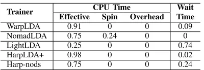
Figure 6: Distributed Performance. Columns 1 to 4, enwiki (K= 10000) with 8x16(nodes×threads) in row 1, clueweb30b (K = 5000) with 40×16 in row 2. Column 5 shows plots speedup versus node count with 16 threads each. The initial word-topic model size is 2.6GB for enwiki and 12.7GB for clueweb30b.
of hundreds of milliseconds make the overhead ratio appear high. As seen in the charts, HarpLDA+ demonstrates the best load balance and a small overhead. WarpLDA is excluded in this experiment because it is implemented with OpenMP and thread log can not be added.
3) Distributed Parallel Efficiency: In this section, we
test the LDA trainers in distributed mode. WarpLDA is not included because the official source code release does not support distributed mode. Moreover, we expect that the distributed design presented in its paper might not scale well because of the need to exchange a much larger modelZ in each iteration among all the workers. F+NomadLDA runs on an InfiniBand network directly supported by mvapich2, but lightlda runs on IPoIB (TCP/IP protocol on InfiniBand network) supported by mpich2, and as a Java application, HarpLDA+ runs on IPoIB too. This means F+NomadLDA can potentially utilize a bandwidth which is at least two times larger in these experiments and is easier to scale.
As shown in Fig. 6, column 1 represents convergence speed, where HarpLDA+ has the best overall performance. In column 2 of Convergence Time Ratio, we calculate the speedup in time of other trainers with respect to HarpLDA+, defined as the ratio of the training time to reach a given Model Log-Likelihood which is the abscissa of the graph.
HarpLDA+ is more than 6x faster than LightLDA, 2x faster than NomadLDA and about 50% slower when timer control is not used. In columns 3 and 4, Load Balance of
Computation and Overhead, HarpLDA+ demonstrates
sig-nificant differences from Harp-notimer, which is the factor behind the boost in performance.
LightLDA, as an asynchronous approach, has less prob-lems of load imbalance than the synchronized approaches. The default staleness is set to one which can tolerate any performance undulations only if the lag of the local model replica is less than two iterations. This mechanism is
effective in order to provide stability and good scalability for different cluster configurations. This is showcased in column 5. On the other hand, LightLDA has a lower convergence rate stemmed from its asynchronous design and is less efficient during the multi-threading parallel implementation. F+NomadLDA is observed to have the most load imbal-ance problems and also exhibits a very high overhead ratio. In the ewniki 10K experiment, the overhead even reaches 90%, i.e., most of the workers are waiting for data. When using a rotation architecture and running directly on the InifiBand network, this result is not expected. One possible reason for this is the task granularity. It takes very small granularity to schedule on each column of the word-topic model, which seems to have a large overhead, especially whenK increases to a large number.
4) Communication Intensive Case Study: The following
experiment runs on the bigram dataset, which has a 20 million vocabulary size that is used to test the special communication intensive case in the distributed mode. We set the parameter of the bound in HarpLDA+ to [150%, 350%] to overlap the communication time in this special case, i.e., the dynamic scheduler keeps assigning those sampled blocks to free threads until the timer is timeout. This trainer is named Harp-repeat.
0 2000 4000 6000 8000 10000 Training Time (s) 2.5 2.4 2.3 2.2 2.1 2.0 1.9 1.8 1.7 1.6 Model Log-likelihood
1e10(a) Convergence Speed
HarpLDA+ Harp-notimer Harp-repeat LightLDA F+NomadLDA
0 50 100 150 200
Epoch Number 2.5 2.4 2.3 2.2 2.1 2.0 1.9 1.8 1.7 1.6 Model Log-likelihood
1e10(b) Convergence Rate
-0.24-0.21-0.18-0.18-0.17-0.17-0.17-0.17-0.17 Model Log-Likelihood(x1e+11) 0 2 4 6 8 10 Speedup
(c) Convergence Time Ratio
0 2000 4000 6000 8000 10000 Training Time (s) 0.0 0.2 0.4 0.6 0.8 1.0
Overhead Ratio Per Iteration
[image:9.612.64.288.71.241.2](d) Overhead
Figure 7: Performance on bigram with 10×8 K=500
exchanged.
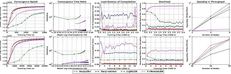
5) Straggler Case Study: The notion of a straggler is
a situation in cloud computations, where some nodes are significantly slower than others in a job for different reasons. In our experiment on the HPC cluster, we also encounter stragglers more often than expected.
0 5000 10000 15000 20000 Training Time (s) 3.0 2.8 2.6 2.4 2.2 2.0 1.8 1.6 1.4 Model Log-likelihood
1e11(a) Convergence Speed
0 2000 4000 6000 8000 10000 Training Time (s) 0 1 2 3 4 5 6 7 Throughput (tokens/s)
1e8 (b) Throughput
0 2000 4000 6000 8000 10000 Training Time (s) 0.0 0.2 0.4 0.6 0.8 1.0 1.2 1.4
CV of Computation Time
(c) Load Balance
HarpLDA+ Harp-notimer HarpLDA+-normal LightLDA F+NomadLDA
0 2000 4000 6000 8000 10000 Training Time (s) 0.0 0.2 0.4 0.6 0.8 1.0
Overhead Ratio Per Iteration
(d) Overhead
Figure 8: Straggler Test on clueweb30b with 40×16 K=5000
In Fig. 8, all the trainers except for HarpLDA+ have been greatly affected by stragglers. When the CV value increases up to around 1.0, the overhead ratio increases more than 80%, throughput drops sharply, and as a result the overall performance drops sharply. For instance, the task does not even converge in 60,000(s) time where a normal run needs about 10,000(s). LightLDA benefits by its SSP design to represent a stable and scaleable trainer in a cluster with minor variances. However, it cannot handle large variances such as the straggler, in which case it stalls. In contrast, F+NomadLDA has a load balance scheduler which is designed to deal with these kinds of situations. When some nodes are detected to be slow and the number of tasks
in its task queue is too large, the scheduler will decrease the probability of sending a new model to the node. However, the performance results are poor due to implementation issues. HarpLDA+ demonstrates a stable performance in the case of straggler. The speedup on the convergence speed of a normal run without a straggler (HarpLDA+-normal) is about 1.25, which means losing about 25% performance when a straggler occurs.
6) Large Model Case Study: Finally, we test the trainers
on very large models, with K set to 100 thousand and 1 million respectively. F+NomadLDA fails in such settings with out-of-memory errors.
0 50 100 150 200 250
Training Time (1000 s) 3.2 3.0 2.8 2.6 2.42.2 2.0 1.8 1.6 1.4 Model Log-likelihood
1e11 (a) K=100K
HarpLDA+ LightLDA-16 LightLDA-128
0 50 100 150 200 250 300 350 400 450 Training Time (1000 s) 3.4 3.2 3.0 2.8 2.6 2.4 2.2 2.0 1.8 1.6 Model Log-likelihood
1e11 (b) K=1M
[image:9.612.322.549.228.311.2]HarpLDA+ LightLDA-16 LightLDA-128
Figure 9: Big Model Test on clueweb30b with 30×30
For Convergence Speed in Fig. 9b, when K increases to 1 million, LightLDA runs much faster than HarpLDA+ due to time complexity of O(1) in the MH sampling algorithm. However this only happens at the beginning of the training phase. Afterwards it slows down and is surpassed by HarpLDA+ because of its ineffectiveness of computation, despite using a very large MH step parameter such as 128 in Fig. 9. In this big model experiment, HarpLDA+ demon-strates impressive performance, given that the algorithm has a time complexity ofO(Kd+Kw)while that of LightLDA
isO(1).
VI. CONCLUSIONS ANDFUTUREWORK
In this paper, we investigate the system design of large scale LDA trainers with a focus on parallel efficiency. Based on these, we introduce HarpLDA+, selecting the Rotation architecture and proposing a new synchronized LDA training system with reduced overhead. This entails a two level parallelism design, in which a dynamic scheduler is used for multi-threading, while rotation with timer control is used for distributed parallelism. Through extensive experiments, we demonstrate that the HarpLDA+ outperforms the other approaches in scaling and stability. We note that all 4 train-ing systems betrain-ing evaluated are compared on the identical Haswell cluster with the same configuration.
From HarpLDA+, we’ve gained useful insights in design-ing a large scale Machine Learndesign-ing system.
[image:9.612.63.291.366.533.2]seen in Tables I and III. The choices of data structures and parallel system design are critical for good perfor-mance in our Java HarpLDA+, as shown in Figures 4 and 6.
• Asynchronous parallel designs are favorable for scala-bility and robustness. However, with increasing paral-lelism and computation capacity provided by manycore and GPU servers, synchronized parallel designs can achieve better performance on a moderate sized cluster for big data problems in Table II.
Incorporating more parallelism, such as vectorization, into LDA trainers can be further explored in future work. Also, the similarity between LDA-CGS trainer and MF-SGD trainer implies some intrinsic relationship between these two large families of Machine Learning algorithms , which are potential future directions to explore.
VII. ACKNOWLEDGMENTS
We gratefully acknowledge support from the Intel Paral-lel Computing Center (IPCC) Grant, NSF 1443054 CIF21 DIBBs 1443054 Grant, NSF OCI 1149432 CAREER Grant and Indiana University Precision Health Initiative. We also appreciate the system support offered by FutureSystems.
REFERENCES
[1] D. M. Blei, A. Y. Ng, and M. I. Jordan, “Latent dirichlet
allocation,”J. Mach. Learn. Res., vol. 3, pp. 993–1022, 2003.
[2] T. L. Griffiths and M. Steyvers, “Finding scientific topics,” Proceedings of the National academy of Sciences of the United States of America, vol. 101, no. Suppl 1, pp. 5228– 5235, 2004.
[3] D. Newman, A. Asuncion, P. Smyth, and M. Welling,
“Dis-tributed Algorithms for Topic Models,”J. Mach. Learn. Res.,
vol. 10, pp. 1801–1828, Dec. 2009.
[4] Y. Wang, H. Bai, M. Stanton, W.-Y. Chen, and E. Y. Chang, “Plda: Parallel latent dirichlet allocation for
large-scale applications,” inAlgorithmic Aspects in Information and
Management. Springer, 2009, pp. 301–314.
[5] P. Smyth, M. Welling, and A. U. Asuncion, “Asynchronous
distributed learning of topic models,” inAdvances in Neural
Information Processing Systems, 2009, pp. 81–88.
[6] A. Smola and S. Narayanamurthy, “An architecture for
par-allel topic models,”Proc. VLDB Endow., vol. 3, no. 1-2, pp.
703–710, Sep. 2010.
[7] A. Ahmed, M. Aly, J. Gonzalez, S. Narayanamurthy, and A. J. Smola, “Scalable inference in latent variable models,”
inProceedings of the fifth ACM international conference on
Web search and data mining. ACM, 2012, pp. 123–132.
[8] M. Li, D. G. Andersen, J. W. Park, A. J. Smola, A. Ahmed, V. Josifovski, J. Long, E. J. Shekita, and B.-Y. Su, “Scaling distributed machine learning with the parameter server,” in Operating Systems Design and Implementation (OSDI), 2014.
[9] Q. Ho, J. Cipar, H. Cui, S. Lee, J. K. Kim, P. B. Gibbons, G. A. Gibson, G. Ganger, and E. P. Xing, “More effective dis-tributed ml via a stale synchronous parallel parameter server,”
in Advances in neural information processing systems, pp.
1223–1231.
[10] F. Yan, N. Xu, and Y. Qi, “Parallel inference for latent
dirichlet allocation on graphics processing units,” inAdvances
in Neural Information Processing Systems, 2009, pp. 2134– 2142.
[11] S. Lee, J. K. Kim, X. Zheng, Q. Ho, G. A. Gibson, and E. P. Xing, “On model parallelization and scheduling strategies
for distributed machine learning,” in Advances in Neural
Information Processing Systems, 2014, pp. 2834–2842.
[12] J. K. Kim, Q. Ho, S. Lee, X. Zheng, W. Dai, G. A. Gibson, and E. P. Xing, “STRADS: a distributed framework for
scheduled model parallel machine learning,” inProceedings
of the Eleventh European Conference on Computer Systems. ACM, 2016, p. 5.
[13] B. Zhang, B. Peng, and J. Qiu, “High performance lda
through collective model communication optimization,”
Pro-cedia Computer Science, vol. 80, pp. 86–97, 2016.
[14] H.-F. Yu, C.-J. Hsieh, H. Yun, S. V. N. Vishwanathan, and I. S. Dhillon, “A scalable asynchronous distributed algorithm
for topic modeling,” inProceedings of the 24th International
Conference on World Wide Web. ACM, 2015, pp. 1340–
1350.
[15] H. Yun, H.-F. Yu, C.-J. Hsieh, S. V. N. Vishwanathan, and I. Dhillon, “NOMAD: Non-locking, stOchastic Multi-machine algorithm for Asynchronous and Decentralized
ma-trix completion,” Proceedings of the VLDB Endowment,
vol. 7, no. 11, pp. 975–986, 2014.
[16] L. Yao, D. Mimno, and A. McCallum, “Efficient methods for topic model inference on streaming document collections,”
in Proceedings of the 15th ACM SIGKDD international
conference on Knowledge discovery and data mining, ser.
KDD ’09. ACM, pp. 937–946.
[17] A. Q. Li, A. Ahmed, S. Ravi, and A. J. Smola, “Reducing the
sampling complexity of topic models,” inProceedings of the
20th ACM SIGKDD international conference on Knowledge
discovery and data mining. ACM, 2014, pp. 891–900.
[18] J. Yuan, F. Gao, Q. Ho, W. Dai, J. Wei, X. Zheng, E. P. Xing, T.-Y. Liu, and W.-Y. Ma, “LightLDA: Big Topic Models on
Modest Compute Clusters,”arXiv preprint arXiv:1412.1576,
2014.
[19] J. Chen, K. Li, J. Zhu, and W. Chen, “WarpLDA: A Cache Efficient O(1) Algorithm for Latent Dirichlet Allocation,” Proc. VLDB Endow., vol. 9, no. 10, pp. 744–755, Jun. 2016.
[20] W.-S. Chin, Y. Zhuang, Y.-C. Juan, and C.-J. Lin, “A Fast Par-allel Stochastic Gradient Method for Matrix Factorization in
Shared Memory Systems,”ACM Transactions on Intelligent
Systems and Technology (TIST), vol. 6, no. 1, p. 2, 2015.
[21] B. D. He, C. M. De Sa, I. Mitliagkas, and C. R, “Scan Order in Gibbs Sampling: Models in Which it Matters and
Bounds on How Much,” inAdvances In Neural Information