ESSENTIALS OF
ERROR-CONTROL
CODING
Jorge Castiñeira Moreira
University of Mar del Plata, ArgentinaPatrick Guy Farrell
Lancaster University, UKESSENTIALS OF
ERROR-CONTROL
CODING
ESSENTIALS OF
ERROR-CONTROL
CODING
Jorge Castiñeira Moreira
University of Mar del Plata, ArgentinaPatrick Guy Farrell
Lancaster University, UKTelephone (+44) 1243 779777
Email (for orders and customer service enquiries): [email protected] Visit our Home Page on www.wiley.com
All Rights Reserved. No part of this publication may be reproduced, stored in a retrieval system or transmitted in any form or by any means, electronic, mechanical, photocopying, recording, scanning or otherwise, except under the terms of the Copyright, Designs and Patents Act 1988 or under the terms of a licence issued by the Copyright Licensing Agency Ltd, 90 Tottenham Court Road, London W1T 4LP, UK, without the permission in writing of the Publisher. Requests to the Publisher should be addressed to the Permissions Department, John Wiley & Sons Ltd, The Atrium, Southern Gate, Chichester, West Sussex PO19 8SQ, England, or emailed to [email protected], or faxed to (+44) 1243 770620.
Designations used by companies to distinguish their products are often claimed as trademarks. All brand names and product names used in this book are trade names, service marks, trademarks or registered trademarks of their respective owners. The Publisher is not associated with any product or vendor mentioned in this book. This publication is designed to provide accurate and authoritative information in regard to the subject matter covered. It is sold on the understanding that the Publisher is not engaged in rendering professional services. If professional advice or other expert assistance is required, the services of a competent professional should be sought.
Other Wiley Editorial Offices
John Wiley & Sons Inc., 111 River Street, Hoboken, NJ 07030, USA Jossey-Bass, 989 Market Street, San Francisco, CA 94103-1741, USA Wiley-VCH Verlag GmbH, Boschstr. 12, D-69469 Weinheim, Germany
John Wiley & Sons Australia Ltd, 42 McDougall Street, Milton, Queensland 4064, Australia John Wiley & Sons (Asia) Pte Ltd, 2 Clementi Loop #02-01, Jin Xing Distripark, Singapore 129809 John Wiley & Sons Canada Ltd, 6045 Freemont Blvd, Mississauga, ONT, L5R 4J3, Canada
Wiley also publishes its books in a variety of electronic formats. Some content that appears in print may not be available in electronic books.
British Library Cataloguing in Publication Data
A catalogue record for this book is available from the British Library ISBN-13 978-0-470-02920-6 (HB)
ISBN-10 0-470-02920-X (HB)
Typeset in 10/12pt Times by TechBooks, New Delhi, India.
Printed and bound in Great Britain by Antony Rowe Ltd, Chippenham, England.
This book is printed on acid-free paper responsibly manufactured from sustainable forestry in which at least two trees are planted for each one used for paper production.
We dedicate this book to
my son Santiago José,
Melisa and Belén,
Maria, Isabel, Alejandra and Daniel,
and the memory of my Father.
J.C.M.
and to all my families and friends.
P.G.F.
Contents
Preface xiii
Acknowledgements xv
List of Symbols xvii
Abbreviations xxv
1 Information and Coding Theory 1
1.1 Information 3
1.1.1 A Measure of Information 3
1.2 Entropy and Information Rate 4
1.3 Extended DMSs 9
1.4 Channels and Mutual Information 10
1.4.1 Information Transmission over Discrete Channels 10
1.4.2 Information Channels 10
1.5 Channel Probability Relationships 13
1.6 The A Priori and A Posteriori Entropies 15
1.7 Mutual Information 16
1.7.1 Mutual Information: Definition 16
1.7.2 Mutual Information: Properties 17
1.8 Capacity of a Discrete Channel 21
1.9 The Shannon Theorems 22
1.9.1 Source Coding Theorem 22
1.9.2 Channel Capacity and Coding 23
1.9.3 Channel Coding Theorem 25
1.10 Signal Spaces and the Channel Coding Theorem 27
1.10.1 Capacity of the Gaussian Channel 28
1.11 Error-Control Coding 32
1.12 Limits to Communication and their Consequences 34
Bibliography and References 38
Problems 38
2 Block Codes 41
2.1 Error-Control Coding 41
2.2 Error Detection and Correction 41
2.2.1 Simple Codes: The Repetition Code 42
2.3 Block Codes: Introduction and Parameters 43
2.4 The Vector Space over the Binary Field 44
2.4.1 Vector Subspaces 46
2.4.2 Dual Subspace 48
2.4.3 Matrix Form 48
2.4.4 Dual Subspace Matrix 49
2.5 Linear Block Codes 50
2.5.1 Generator Matrix G 51
2.5.2 Block Codes in Systematic Form 52
2.5.3 Parity Check Matrix H 54
2.6 Syndrome Error Detection 55
2.7 Minimum Distance of a Block Code 58
2.7.1 Minimum Distance and the Structure of the H Matrix 58 2.8 Error-Correction Capability of a Block Code 59
2.9 Syndrome Detection and the Standard Array 61
2.10 Hamming Codes 64
2.11 Forward Error Correction and Automatic Repeat ReQuest 65
2.11.1 Forward Error Correction 65
2.11.2 Automatic Repeat ReQuest 68
2.11.3 ARQ Schemes 69
2.11.4 ARQ Scheme Efficiencies 71
2.11.5 Hybrid-ARQ Schemes 72
Bibliography and References 76
Problems 77
3 Cyclic Codes 81
3.1 Description 81
3.2 Polynomial Representation of Codewords 81
3.3 Generator Polynomial of a Cyclic Code 83
3.4 Cyclic Codes in Systematic Form 85
3.5 Generator Matrix of a Cyclic Code 87
3.6 Syndrome Calculation and Error Detection 89
3.7 Decoding of Cyclic Codes 90
3.8 An Application Example: Cyclic Redundancy Check Code for the Ethernet Standard 92
Bibliography and References 93
Problems 94
4 BCH Codes 97
4.1 Introduction: The Minimal Polynomial 97
4.2 Description of BCH Cyclic Codes 99
4.2.1 Bounds on the Error-Correction Capability of a BCH Code: The Vandermonde
4.3 Decoding of BCH Codes 104 4.4 Error-Location and Error-Evaluation Polynomials 105
4.5 The Key Equation 107
4.6 Decoding of Binary BCH Codes Using the Euclidean Algorithm 108
4.6.1 The Euclidean Algorithm 108
Bibliography and References 112
Problems 112
5 Reed–Solomon Codes 115
5.1 Introduction 115
5.2 Error-Correction Capability of RS Codes: The Vandermonde Determinant 117
5.3 RS Codes in Systematic Form 119
5.4 Syndrome Decoding of RS Codes 120
5.5 The Euclidean Algorithm: Error-Location and Error-Evaluation Polynomials 122 5.6 Decoding of RS Codes Using the Euclidean Algorithm 125
5.6.1 Steps of the Euclidean Algorithm 127
5.7 Decoding of RS and BCH Codes Using the Berlekamp–Massey Algorithm 128 5.7.1 B–M Iterative Algorithm for Finding the Error-Location Polynomial 130
5.7.2 B–M Decoding of RS Codes 133
5.7.3 Relationship Between the Error-Location Polynomials of the Euclidean and
B–M Algorithms 136
5.8 A Practical Application: Error-Control Coding for the Compact Disk 136
5.8.1 Compact Disk Characteristics 136
5.8.2 Channel Characteristics 138
5.8.3 Coding Procedure 138
5.9 Encoding for RS codes CRS(28, 24), CRS(32, 28) and CRS(255, 251) 139 5.10 Decoding of RS Codes CRS(28, 24) and CRS(32, 28) 142
5.10.1 B–M Decoding 142
5.10.2 Alternative Decoding Methods 145
5.10.3 Direct Solution of Syndrome Equations 146
5.11 Importance of Interleaving 148
Bibliography and References 152
Problems 153
6 Convolutional Codes 157
6.1 Linear Sequential Circuits 158
6.2 Convolutional Codes and Encoders 158
6.3 Description in the D-Transform Domain 161
6.4 Convolutional Encoder Representations 166
6.4.1 Representation of Connections 166
6.4.2 State Diagram Representation 166
6.4.3 Trellis Representation 168
6.5 Convolutional Codes in Systematic Form 168
6.6 General Structure of Finite Impulse Response and Infinite Impulse Response FSSMs 170
6.6.1 Finite Impulse Response FSSMs 170
6.7 State Transfer Function Matrix: Calculation of the Transfer Function 172
6.7.1 State Transfer Function for FIR FSSMs 172
6.7.2 State Transfer Function for IIR FSSMs 173
6.8 Relationship Between the Systematic and the Non-Systematic Forms 175 6.9 Distance Properties of Convolutional Codes 177 6.10 Minimum Free Distance of a Convolutional Code 180
6.11 Maximum Likelihood Detection 181
6.12 Decoding of Convolutional Codes: The Viterbi Algorithm 182
6.13 Extended and Modified State Diagram 185
6.14 Error Probability Analysis for Convolutional Codes 186
6.15 Hard and Soft Decisions 189
6.15.1 Maximum Likelihood Criterion for the Gaussian Channel 192
6.15.2 Bounds for Soft-Decision Detection 194
6.15.3 An Example of Soft-Decision Decoding of Convolutional Codes 196 6.16 Punctured Convolutional Codes and Rate-Compatible Schemes 200
Bibliography and References 203
Problems 205
7 Turbo Codes 209
7.1 A Turbo Encoder 210
7.2 Decoding of Turbo Codes 211
7.2.1 The Turbo Decoder 211
7.2.2 Probabilities and Estimates 212
7.2.3 Symbol Detection 213
7.2.4 The Log Likelihood Ratio 214
7.3 Markov Sources and Discrete Channels 215
7.4 The BCJR Algorithm: Trellis Coding and Discrete Memoryless Channels 218
7.5 Iterative Coefficient Calculation 221
7.6 The BCJR MAP Algorithm and the LLR 234
7.6.1 The BCJR MAP Algorithm: LLR Calculation 235
7.6.2 Calculation of Coefficientsγi(u,u) 236
7.7 Turbo Decoding 239
7.7.1 Initial Conditions of Coefficientsαi−1(u) andβi(u) 248
7.8 Construction Methods for Turbo Codes 249
7.8.1 Interleavers 249
7.8.2 Block Interleavers 250
7.8.3 Convolutional Interleavers 250
7.8.4 Random Interleavers 251
7.8.5 Linear Interleavers 253
7.8.6 Code Concatenation Methods 253
7.8.7 Turbo Code Performance as a Function of Size and Type of Interleaver 257 7.9 Other Decoding Algorithms for Turbo Codes 257
7.10 EXIT Charts for Turbo Codes 257
7.10.1 Introduction to EXIT Charts 258
7.10.2 Construction of the EXIT Chart 259
Bibliography and References 269
Problems 271
8 Low-Density Parity Check Codes 277
8.1 Different Systematic Forms of a Block Code 278
8.2 Description of LDPC Codes 279
8.3 Construction of LDPC Codes 280
8.3.1 Regular LDPC Codes 280
8.3.2 Irregular LDPC Codes 281
8.3.3 Decoding of LDPC Codes: The Tanner Graph 281
8.4 The Sum–Product Algorithm 282
8.5 Sum–Product Algorithm for LDPC Codes: An Example 284 8.6 Simplifications of the Sum–Product Algorithm 297
8.7 A Logarithmic LDPC Decoder 302
8.7.1 Initialization 302
8.7.2 Horizontal Step 302
8.7.3 Vertical Step 304
8.7.4 Summary of the Logarithmic Decoding Algorithm 305
8.7.5 Construction of the Look-up Tables 306
8.8 Extrinsic Information Transfer Charts for LDPC Codes 306
8.8.1 Introduction 306
8.8.2 Iterative Decoding of Block Codes 310
8.8.3 EXIT Chart Construction for LDPC Codes 312
8.8.4 Mutual Information Function 312
8.8.5 EXIT Chart for the SND 314
8.8.6 EXIT Chart for the PCND 315
8.9 Fountain and LT Codes 317
8.9.1 Introduction 317
8.9.2 Fountain Codes 318
8.9.3 Linear Random Codes 318
8.9.4 Luby Transform Codes 320
8.10 LDPC and Turbo Codes 322
Bibliography and References 323
Problems 324
Appendix A: Error Probability in the Transmission of Digital Signals 327
Appendix B: Galois Fields GF(q) 339
Answers to Problems 351
Preface
The subject of this book is the detection and correction of errors in digital information. Such errors almost inevitably occur after the transmission, storage or processing of information in digital (mainly binary) form, because of noise and interference in communication channels, or imperfections in storage media, for example. Protecting digital information with a suitable error-control code enables the efficient detection and correction of any errors that may have occurred.
Error-control codes are now used in almost the entire range of information communication, storage and processing systems. Rapid advances in electronic and optical devices and systems have enabled the implementation of very powerful codes with close to optimum error-control performance. In addition, new types of code, and new decoding methods, have recently been developed and are starting to be applied. However, error-control coding is complex, novel and unfamiliar, not yet widely understood and appreciated. This book sets out to provide a clear description of the essentials of the topic, with comprehensive and up-to-date coverage of the most useful codes and their decoding algorithms. The book has a practical engineering and information technology emphasis, but includes relevant background material and fundamental theoretical aspects. Several system applications of error-control codes are described, and there are many worked examples and problems for the reader to solve.
The book is an advanced text aimed at postgraduate and third/final year undergraduate students of courses on telecommunications engineering, communication networks, electronic engineering, computer science, information systems and technology, digital signal processing, and applied mathematics, and for engineers and researchers working in any of these areas. The book is designed to be virtually self-contained for a reader with any of these backgrounds. Enough information and signal theory, and coding mathematics, is included to enable a full understanding of any of the error-control topics described in the book.
Chapter 1 provides an introduction to information theory and how it relates to error-control coding. The theory defines what we mean by information, determines limits on the capacity of an information channel and tells us how efficient a code is at detecting and correcting errors. Chapter 2 describes the basic concepts of error detection and correction, in the context of the parameters, encoding and decoding of some simple binary block error-control codes. Block codes were the first type of error-control code to be discovered, in the decade from about 1940 to 1950. The two basic ways in which error coding is applied to an information system are also described: forward error correction and retransmission error control. A particularly useful kind of block code, the cyclic code, is introduced in Chapter 3, together with an example of a practical application, the cyclic redundancy check (CRC) code for the Ethernet standard. In Chapters 4 and 5 two very effective and widely used classes of cyclic codes are described,
the Bose–Chaudhuri–Hocquenghem (BCH) and Reed–Solomon (RS) codes, named after their inventors. BCH codes can be binary or non-binary, but the RS codes are non-binary and are particularly effective in a large number of error-control scenarios. One of the best known of these, also described in Chapter 5, is the application of RS codes to error correction in the compact disk (CD).
Not long after the discovery of block codes, a second type of error-control codes emerged, initially called recurrent and later convolutional codes. Encoding and decoding even a quite powerful convolutional code involves rather simple, repetitive, quasi-continuous processes, applied on a very convenient trellis representation of the code, instead of the more complex block processing that seems to be required in the case of a powerful block code. This makes it relatively easy to use maximum likelihood (soft-decision) decoding with convolutional codes, in the form of the optimum Viterbi algorithm (VA). Convolutional codes, their trellis and state diagrams, soft-decision detection, the Viterbi decoding algorithm, and practical punctured and rate-compatible coding schemes are all presented in Chapter 6. Disappointingly, however, even very powerful convolutional codes were found to be incapable of achieving performances close to the limits first published by Shannon, the father of information theory, in 1948. This was still true even when very powerful combinations of block and convolutional codes, called concatenated codes, were devised. The breakthrough, by Berrou, Glavieux and Thitimajshima in 1993, was to use a special kind of interleaved concatenation, in conjunction with iterative soft-decision decoding. All aspects of these very effective coding schemes, called turbo codes because of the supercharging effect of the iterative decoding algorithm, are fully described in Chapter 7.
The final chapter returns to the topic of block codes, in the form of low-density parity check (LDPC) codes. Block codes had been found to have trellis representations, so that they could be soft-decision decoded with performances almost as good as those of convolutional codes. Also, they could be used in effective turbo coding schemes. Complexity remained a problem, however, until it was quite recently realized that a particularly simple class of codes, the LDPC codes discovered by Gallager in 1962, was capable of delivering performances as good or better than those of turbo codes when decoded by an appropriate iterative algorithm. All aspects of the construction, encoding, decoding and performance of LDPC codes are fully described in Chapter 8, together with various forms of LDPC codes which are particularly effective for use in communication networks.
Appendix A shows how to calculate the error probability of digital signals transmitted over additive white Gaussian noise (AWGN) channels, and Appendix B introduces various topics in discrete mathematics. These are followed by a list of the answers to the problems located at the end of each chapter. Detailed solutions are available on the website associated with this book, which can be found at the following address:
http://elaf1.fi.mdp.edu.ar/Error Control
Acknowledgements
We are very grateful for all the help, support and encouragement we have had during the writing of this book, from our colleagues past and present, from many generations of research assistants and students, from the reviewers and from our families and friends. We particularly thank Damian Levin and Leonardo Arnone for their contributions to Chapters 7 and 8, respectively; Mario Blaum, Rolando Carrasco, Evan Ciner, Bahram Honary, Garik Markarian and Robert McEliece for stimulating discussions and very welcome support; and Sarah Hinton at John Wiley & Sons, Ltd who patiently waited for her initial suggestion to bear fruit.
List of Symbols
Chapter 1
α probability of occurrence of a source symbol (Chapter 1) δ, ε arbitrary small numbers
σ standard deviation
(α) entropy of the binary source evaluated using logs to base 2
B bandwidth of a channel
C capacity of a channel, bits per second
c code vector, codeword
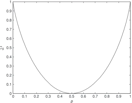
Cs capacity of a channel, bits per symbol
d,i,j,k,l,m,n integer numbers Eb average bit energy
Eb/N0 average bit energy-to-noise power spectral density ratio
H (X ) entropy in bits per second H (Xn) entropy of an extended source
H (X/yj) a posteriori entropy
H (X/Y ) equivocation H (Y/X ) noise entropy
Hb(X ) entropy of a discrete source calculated in logs to base b
I (xi,yj) mutual information of xi,yj
I (X,Y ) average mutual information Ii information of the symbol xi
M number of symbols of a discrete source
n length of a block of information, block code length N0/2 noise power spectral density
nf large number of emitted symbols
p error probability of the BSC or BEC
P power of a signal
P(xi)=Pi probability of occurrence of the symbol xi
P(xi/yj) backward transition probability
P(xi,yj) joint probability of xi,yj
P(X/Y) conditional probability of vector X given vector Y
Pij=P(yj/xi) conditional probability of symbol yj given xi, also transition probability
of a channel; forward transition probability
Pke error probability, in general k identifies a particular index
PN noise power
Pch transition probability matrix
Qi a probability
R information rate
rb bit rate
s,r symbol rate
S/N signal-to-noise ratio
T signal time duration
Ts sampling period
W bandwidth of a signal
x variable in general, also a particular value of random variable X X random variable (Chapters 1, 7 and 8), and variable of a polynomial
expression (Chapters 3, 4 and 5) x(t),s(t) signals in the time domain
xi value of a source symbol, also a symbol input to a channel
xk=x(kTs) sample of signal x(t)
||X|| norm of vector X
yj value of a symbol, generally a channel output
Chapter 2
A amplitude of a signal or symbol Ai number of codewords of weight i
D stopping time (Chapter 2); D-transform domain variable d(ci,cj) Hamming distance between two code vectors
Di set of codewords
dmin minimum distance of a code e error pattern vector
F a field
f (m) redundancy obtained, code C0, hybrid ARQ
G generator matrix
gi row vector of generator matrix G gij element of generator matrix
GF(q) Galois or finite field
H parity check matrix
hj row vector of parity check matrix H k,n message and code lengths in a block code l number of detectable errors in a codeword m random number of transmissions (Chapter 2)
m message vector
N integer number
P(i,n) probability of i erroneous symbols in a block of n symbols
P parity check submatrix
pij element of the parity check submatrix
Pbe bit error rate (BER)
Pret probability of a retransmission in ARQ schemes
PU(E) probability of undetected errors
Pwe word or code vector error probability
q power of a prime number pprime
q(m) redundancy obtained, code C1, hybrid ARQ
r received vector
Rc code rate
S subspace of a vector space V (Chapter 2)
S syndrome vector (Chapters 2–5, 8)
si component of a syndrome vector (Chapters 2–5, 8)
Sd dual subspace of the subspace S
t number of correctable errors in a codeword
td transmission delay
Tw duration of a word
u=(u1,u2, . . .un−1) vector of n components
V a vector space
Vn vector space of dimension n
w(c) Hamming weight of code vector c
Chapter 3
αi primitive element of Galois field GF(q) (Chapters 4 and 5,
Appendix B)
βi root of minimal polynomial (Chapters 4 and 5, Appendix B)
c(X ) code polynomial
c(i )(X ) i-position right-shift rotated version of the polynomial c(X )
e(X ) error polynomial
g(X ) generator polynomial
m(X ) message polynomial
p(X ) remainder polynomial (redundancy polynomial in systematic form) (Chapter 3),
pi(X ) primitive polynomial
r level of redundancy and degree of the generator polynomial (Chapters 3 and 4 only)
r (X ) received polynomial
S(X ) syndrome polynomial
Chapter 4
βl, αjl error-location numbers i(X ) minimal polynomial
ej h value of an error
jl position of an error in a received vector
qi,ri,si,ti auxiliary numbers in the Euclidean algorithm (Chapters 4
and 5)
ri(X ),si(X ),ti(X ) auxiliary polynomials in the Euclidean algorithm (Chapters 4
and 5)
W (X ) error-evaluation polynomial
Chapter 5
ρ a previous step with respect toμin the Berlekamp–Massey (B–M) algorithm
σ(μ)
BM(X ) error-location polynomial, B–M algorithm,μth iteration
dμ μth discrepancy, B–M algorithm
lμ degree of the polynomialσBM(μ)(X ), B–M algorithm
ˆ
m estimate of a message vector
sRS number of shortened symbols in a shortened RS code
Z (X ) polynomial for determining error values in the B–M algorithm
Chapter 6
Ai number of sequences of weight i (Chapter 6)
Ai,j,l number of paths of weight i , of length j , which result from
an input of weight l
bi(T ) sampled value of bi(t), the noise-free signal, at time instant T
C(D) code polynomial expressions in the D domain
ci ith branch of code sequence c
ci n-tuple of coded elements
Cm(D) multiplexed output of a convolutional encoder in the D domain
cji jth code symbol of ci
C( j )(D) output sequence of the j th branch of a convolutional encoder,
in the D domain
ci( j )=(c( j )0 ,c1( j ),c( j )2 , . . .) output sequence of the j th branch of a convolutional encoder df minimum free distance of a convolutional code
dH Hamming distance
G(D) rational transfer function of polynomial expressions in the D domain
G(D) rational transfer function matrix in the D domain
G( j )i (D) impulse response of the j th branch of a convolutional
encoder, in the D domain
H0 hypothesis of the transmission of symbol ‘0’
H1 hypothesis of the transmission of symbol ‘1’
J decoding length
K number of memory units of a convolutional encoder K+1 constraint length of a convolutional code
Ki length of the i th register of a convolutional encoder
L length of a sequence
M(D) message polynomial expressions in the D domain
mi k-tuple of message elements
nA constraint length of a convolutional code, measured in bits
Pp puncturing matrix
S(D) state transfer function
si(k) state sequences in the time domain
si(t) a signal in the time domain
Si(D) state sequences in the D domain Sj=(s0 j,s1 j,s2 j, . . .) state vectors of a convolutional encoder
sr received sequence
sri ith branch of received sequence sr
sr,ji jth symbol of sri
T (X ) generating function of a convolutional code T (X,Y,Z ) modified generating function
ti time instant
Tp puncturing period
Chapter 7
αi(u) forward recursion coefficients of the BCJR algorithm
βi(u) backward recursion coefficients of the BCJR algorithm
λi(u), σi(u,u), γi(u,u) quantities involved in the BCJR algorithm
μ(x) measure or metric of the event x
μ(x,y) joint measure for a pair of random variables X and Y μMAP(x) maximum a posteriori measure or metric of the event x
μML(x) maximum likelihood measure or metric of the event x
μY mean value of random variable Y
π(i ) permutation
σ2
Y variance of a random variable Y
A random variable of a priori estimates D random variable of extrinsic estimates of bits E random variable of extrinsic estimates E(i ) extrinsic estimates for bit i
histE(ξ/X =x) histogram that represents the probability density function
I{.}interleaver permutation pE(ξ/X =x)
IA,I (X ; A) mutual information between the random variables A and X
IE =Tr(IA,Eb/N0) extrinsic information transfer function
J (σ) mutual information function
JMTC number of encoders in a multiple turbo code
J−1(I
A) inverse of the mutual information function
L(x) metric of a given event x
L(bi) log likelihood ratio for bit bi
L(bi/Y),L(bi/Y1n) conditioned log likelihood ratio given the received
sequence Y, for bit bi
Lc measure of the channel signal-to-noise ratio
LcY( j ) channel information for a turbo decoder, j th iteration
Le(bi) extrinsic log likelihood ratio for bit bi
L( j )e (bi) extrinsic log likelihood ratio for bit bi, j -th iteration
L( j )(b
i/Y) conditioned log likelihood ratio given the received
sequence Y, for bit bi, j th iteration
MI×NI size of a block interleaver
nY random variable with zero mean value and varianceσY2
p(x) probability distribution of a discrete random variable p(Xj) source marginal distribution function
pA(ξ/X =x) probability density function of a priori estimates A for X =x
pE(ξ/X=x) probability density function of extrinsic estimates E for
X =x
pMTC the angular coefficient of a linear interleaver
Rj(Yj/Xj) channel transition probability
sMTC linear shift of a linear interleaver
Sij = {Si,Si+1, . . . ,Sj} generic vector or sequence of states of a Hidden Markov
source
u current state value
u previous state value
X=Xn
1 = {X1,X2, . . . ,Xn} vector or sequence of n random variables
Xij = {Xi,Xi+1, . . . ,Xj} generic vector or sequence of random variables
Chapter 8
δQij difference of coefficients Qxij
δRij difference of coefficients Rijx
A and B sparse submatrices of the parity check matrix H (Chapter 8)
A(it)ij a posteriori estimate in iteration number it
d decoded vector
ˆ
d estimated decoded vector
dj symbol nodes
d(i )
c number of symbol nodes or bits related to parity check
node hi
dv( j ) number of parity check equations in which the bit or
d p message packet code vector
dpn message packet in a fountain or linear random code
Ex number of excess packets of a fountain or linear random
code
f+(|z1|,|z2|),f−(|z1|,|z2|) look-up tables for an LDPC decoder implementation with
entries|z1|,|z2|
fjx a priori estimates of the received symbols
Gfr fragment generator matrix
{Gkn} generator matrix of a fountain or linear random code
hi parity check nodes
IE,SND(IA,dv,Eb/N0,Rc) EXIT chart for the symbol node decoder
IE,PCND(IA,dc) EXIT chart for the parity check node decoder
L(b1⊕b2),L(b1)[⊕]L(b2) LLR of an exclusive-OR sum of two bits
Lch=L(0)ch channel LLR
L(it)ij LLR that each parity check node hi sends to each symbol
node djin iteration number it L Qx
ij,L fjx,L Rijx,L Qxj L values for Qxij, fjx, Rijx, Qxj, respectively
|Lz| an L value, that is, the absolute value of the natural log of z
M( j) set of indexes of all the children parity check nodes connected to the symbol node dj
M( j)\i set of indexes of all the children parity check nodes connected to the symbol node dj with the exclusion of
the child parity check node hi
N (i) set of indexes of all the parent symbol nodes connected to the parity check node hi
N (i)\j set of indexes of all the parent symbol nodes connected to the parity check node hiwith the exclusion of the
parent symbol node dj
Nt number of entries of a look-up table for the logarithmic
LDPC decoder
Qxj a posteriori probabilities
Qxij estimate that each symbol node dj sends to each of its
children parity check nodes hiin the sum–product
algorithm Rx
ij estimate that each parity check node hisends to each of its
parent symbol nodes dj in the sum–product algorithm
s number of ‘1’s per column of parity check matrix H (Chapter 8)
t p transmitted packet code vector
tpn transmitted packet in a fountain or linear random code
v number of ‘1’s per row of parity check matrix H (Chapter 8)
z positive real number such that z≤1
Zij(it) LLR that each symbol node djsends to each parity check
Appendix A
τ time duration of a given pulse (Appendix A)
ak amplitude of the symbol k in a digital amplitude modulated signal
NR received noise power
p(t) signal in a digital amplitude modulated transmission Q(k) normalized Gaussian probability density function T duration of the transmitted symbol in a digital
amplitude-modulated signal
SR received signal power
U threshold voltage (Appendix A)
x(t),y(t),n(t) transmitted, received and noise signals, respectively
Appendix B
φ(X ) minimum-degree polynomial
F field
f (X ) polynomial defined over GF(2)
Abbreviations
ACK positive acknowledgement APP a posteriori probability ARQ automatic repeat request AWGN additive white Gaussian noise
BCH Bose, Chaudhuri, Hocquenghem (code) BCJR Bahl, Cocke, Jelinek, Raviv (algorithm) BEC binary erasure channel
BER bit error rate
BM/B–M Berlekamp–Massey (algorithm) BPS/bps bits per second
BSC binary symmetric channel
ch channel
CD compact disk
CIRC cross-interleaved Reed–Solomon code conv convolutional (code)
CRC cyclic redundancy check
dec decoder
deg degree
DMC discrete memoryless channel DMS discrete memoryless source
DRP dithered relatively prime (interleaver)
enc encoder
EFM eight-to-fourteen modulation EXIT extrinsic information transfer FCS frame check sequence FEC forward error correction FIR finite impulse response FSSM finite state sequential machine GF Galois field
HCF/hcf highest common factor IIR infinite impulse response ISI inter-symbol interference
lim limit
LCM/lcm lowest common multiple LDPC low-density parity check (code)
LLR log likelihood ratio LT Luby transform
MAP maximum a posteriori probability ML maximum likelihood
MLD maximum likelihood detection mod modulo
MTC multiple turbo code NAK negative acknowledgement NRZ non-return to zero
ns non-systematic opt optimum
PCND parity check node decoder RCPC rate-compatible punctured code(s) RLL run length limited
RS Reed–Solomon (code)
RSC recursive systematic convolutional (code/encoder) RZ return to zero
1
Information and Coding Theory
In his classic paper ‘A Mathematical Theory of Communication’, Claude Shannon [1] intro-duced the main concepts and theorems of what is known as information theory. Definitions and models for two important elements are presented in this theory. These elements are the binary source (BS) and the binary symmetric channel (BSC). A binary source is a device that generates one of the two possible symbols ‘0’ and ‘1’ at a given rate r,measured in symbols per second. These symbols are called bits (binary digits) and are generated randomly.
The BSC is a medium through which it is possible to transmit one symbol per time unit. However, this channel is not reliable, and is characterized by the error probability p (0≤ p ≤ 1/2) that an output bit can be different from the corresponding input. The symmetry of this channel comes from the fact that the error probability p is the same for both of the symbols involved.
Information theory attempts to analyse communication between a transmitter and a receiver through an unreliable channel, and in this approach performs, on the one hand, an analysis of information sources, especially the amount of information produced by a given source, and, on the other hand, states the conditions for performing reliable transmission through an unreliable channel.
There are three main concepts in this theory:
1. The first one is the definition of a quantity that can be a valid measurement of information, which should be consistent with a physical understanding of its properties.
2. The second concept deals with the relationship between the information and the source that generates it. This concept will be referred to as source information. Well-known information theory techniques like compression and encryption are related to this concept.
3. The third concept deals with the relationship between the information and the unreliable channel through which it is going to be transmitted. This concept leads to the definition of a very important parameter called the channel capacity. A well-known information theory technique called error-correction coding is closely related to this concept. This type of coding forms the main subject of this book.
One of the most used techniques in information theory is a procedure called coding, which is intended to optimize transmission and to make efficient use of the capacity of a given channel.
Essentials of Error-Control Coding Jorge Casti˜neira Moreira and Patrick Guy Farrell
C
2006 John Wiley & Sons, Ltd
Table 1.1 Coding: a codeword for each message
Messages Codewords
s1 101
s2 01
s3 110
s4 000
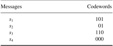
In general terms, coding is a bijective assignment between a set of messages to be transmitted, and a set of codewords that are used for transmitting these messages. Usually this procedure adopts the form of a table in which each message of the transmission is in correspondence with the codeword that represents it (see an example in Table 1.1).
Table 1.1 shows four codewords used for representing four different messages. As seen in this simple example, the length of the codeword is not constant. One important property of a coding table is that it is constructed in such a way that every codeword is uniquely decodable. This means that in the transmission of a sequence composed of these codewords there should be only one possible way of interpreting that sequence. This is necessary when variable-length coding is used.
If the code shown in Table 1.1 is compared with a constant-length code for the same case, constituted from four codewords of two bits, 00, 01, 10, 11, it is seen that the code in Table 1.1 adds redundancy. Assuming equally likely messages, the average number of transmitted bits per symbol is equal to 2.75. However, if for instance symbol s2 were characterized by a
probability of being transmitted of 0.76, and all other symbols in this code were characterized by a probability of being transmitted equal to 0.08, then this source would transmit an average number of bits per symbol of 2.24 bits. As seen in this simple example, a level of compression is possible when the information source is not uniform, that is, when a source generates messages that are not equally likely.
The source information measure, the channel capacity measure and coding are all related by one of the Shannon theorems, the channel coding theorem, which is stated as follows:
If the information rate of a given source does not exceed the capacity of a given channel, then there exists a coding technique that makes possible transmission through this unreliable channel with an arbitrarily low error rate.
This important theorem predicts the possibility of error-free transmission through a noisy or unreliable channel. This is obtained by using coding. The above theorem is due to Claude Shannon [1, 2], and states the restrictions on the transmission of information through a noisy channel, stating also that the solution for overcoming those restrictions is the application of a rather sophisticated coding technique. What is not formally stated is how to implement this coding technique.
A block diagram of a communication system as related to information theory is shown in Figure 1.1.
Source encoder
Noisy channel
Source decoder
Channel decoder Destination
Source Channel
encoder
Figure 1.1 A communication system: source and channel coding
a reliable one. On the other hand, there also exists a source encoder that is designed to make the source information rate approach the channel capacity. The destination is also called the information sink.
Some concepts relating to the transmission of discrete information are introduced in the following sections.
1.1 Information
1.1.1 A Measure of Information
From the point of view of information theory, information is not knowledge, as commonly understood, but instead relates to the probabilities of the symbols used to send messages between a source and a destination over an unreliable channel. A quantitative measure of symbol information is related to its probability of occurrence, either as it emerges from a source or when it arrives at its destination. The less likely the event of a symbol occurrence, the higher is the information provided by this event. This suggests that a quantitative measure of symbol information will be inversely proportional to the probability of occurrence.
Assuming an arbitrary message xiwhich is one of the possible messages from a set a given
discrete source can emit, and P(xi)=Pi is the probability that this message is emitted, the
output of this information source can be modelled as a random variable X that can adopt any of the possible values xi,so that P(X=xi)=Pi. Shannon defined a measure of the information
for the event xiby using a logarithmic measure operating over the base b:
Ii ≡ −logbPi =logb
1 Pi
(1)
The base of the logarithmic measure can be converted by using
loga(x)=logb(x) 1 logb(a)
(2)
If this measure is calculated to base 2, the information is said to be measured in bits. If the measure is calculated using natural logarithms, the information is said to be measured in nats. As an example, if the event is characterized by a probability of Pi =1/2,the corresponding
information is Ii =1 bit. From this point of view, a bit is the amount of information obtained
from one of two possible, and equally likely, events. This use of the term bit is essentially different from what has been described as the binary digit. In this sense the bit acts as the unit of the measure of information.
Some properties of information are derived from its definition: Ii ≥ 0 0≤ Pi ≤1
Ii →0 if Pi →1
Ii > Ij if Pi <Pj
For any two independent source messages xiand xjwith probabilities Piand Pjrespectively,
and with joint probability P(xi,xj)=PiPj,the information of the two messages is the addition
of the information in each message:
Ii j =logb
1 PiPj =
logb 1 Pi +
logb 1 Pj =
Ii+Ij
1.2 Entropy and Information Rate
In general, an information source generates any of a set of M different symbols, which are considered as representatives of a discrete random variable X that adopts any value in the range A= {x1,x2, . . . ,xM}. Each symbol xi has the probability Pi of being emitted and contains
information Ii. The symbol probabilities must be in agreement with the fact that at least one
of them will be emitted, so
M
i=1
Pi =1 (3)
The source symbol probability distribution is stationary, and the symbols are independent and transmitted at a rate of r symbols per second. This description corresponds to a discrete memoryless source (DMS), as shown in Figure 1.2.
Each symbol contains the information Ii so that the set{I1,I2, . . . ,IM}can be seen as a
discrete random variable with average information
Hb(X )= M
i=1
PiIi = M
i=1
Pi logb
1 Pi
Discrete memoryless source
xi , x j, ...
Figure 1.2 A discrete memoryless source
The function so defined is called the entropy of the source. When base 2 is used, the entropy is measured in bits per symbol:
H (X )=
M
i=1
PiIi = M
i=1
Pi log2
1 Pi
bits per symbol (5)
The symbol information value when Pi=0 is mathematically undefined. To solve this
situation, the following condition is imposed: Ii = ∞if Pi =0. Therefore Pilog2
1Pi
=0 (L’Hopital’s rule) if Pi =0. On the other hand, Pilog
1Pi
=0 if Pi =1.
Example 1.1: Suppose that a DMS is defined over the range of X,A= {x1,x2,x3,x4},and
the corresponding probability values for each symbol are P(X =x1)=1/2,P(X=x2)=
P(X =x3)=1/8 and P(X =x4)=1/4.
Entropy for this DMS is evaluated as
H (X )=
M
i=1
Pilog2
1 Pi
= 1
2log2(2)+ 1
8log2(8)+ 1
8log2(8)+ 1 4log2(4)
=1.75 bits per symbol
Example 1.2: A source characterized in the frequency domain with a bandwidth of W = 4000 Hz is sampled at the Nyquist rate, generating a sequence of values taken from the range A= {−2,−1,0,1,2}with the following corresponding set of probabilities12,14,18,161,161 . Calculate the source rate in bits per second.
Entropy is first evaluated as
H (X )=
M
i=1
Pilog2
1 Pi
= 1
2log2(2)+ 1
4log2(4)+ 1 8log2(8)
+2× 1
16log2(16)= 15
8 bits per sample
The minimum sampling frequency is equal to 8000 samples per second, so that the information rate is equal to 15 kbps.
Entropy can be evaluated to a different base by using
Hb(X )=
H (X )
Entropy H (X ) can be understood as the mean value of the information per symbol provided by the source being measured, or, equivalently, as the mean value experienced by an observer before knowing the source output. In another sense, entropy is a measure of the randomness of the source being analysed. The entropy function provides an adequate quantitative measure of the parameters of a given source and is in agreement with physical understanding of the information emitted by a source.
Another interpretation of the entropy function [5] is seen by assuming that if n1 symbols are emitted, n H (X ) bits is the total amount of information emitted. As the source generates r symbols per second, the whole emitted sequence takes n/r seconds. Thus, information will be transmitted at a rate of
n H (X )
(n/r ) bps (7)
The information rate is then equal to
R=r H (X ) bps (8)
The Shannon theorem states that information provided by a given DMS can be coded using binary digits and transmitted over an equivalent noise-free channel at a rate of
rb≥ R symbols or binary digits per second
It is again noted here that the bit is the unit of information, whereas the symbol or binary digit is one of the two possible symbols or signals ‘0’ or ‘1’, usually also called bits.
Theorem 1.1: Let X be a random variable that adopts values in the range A= {x1,
x2, . . . ,xM}and represents the output of a given source. Then it is possible to show that
0≤H (X )≤log2(M) (9)
Additionally,
H (X )=0 if and only if Pi=1 for some i
H (X )=log2(M) if and only if Pi =1
M for every i (10)
The condition 0≤H (X ) can be verified by applying the following: Pilog2(1/Pi)→0 if Pi →0
The condition H (X )≤log2(M) can be verified in the following manner:
Let Q1,Q2, . . . ,QMbe arbitrary probability values that are used to replace terms 1/Pi by
the terms Qi/Piin the expression of the entropy [equation (5)]. Then the following inequality
is used:
0.2 0.4 0.6 0.8 1 1.2 1.4 1.6 1.8 2 –2 –1.5 –1 –0.5 0 0.5 1 x y1,
y2
y2=ln(x)
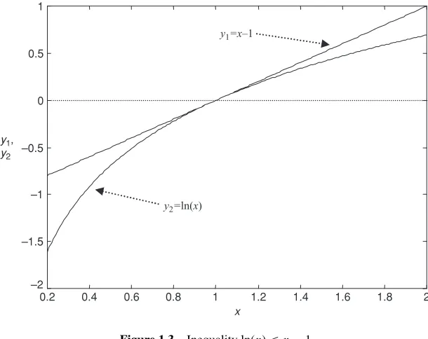
[image:36.432.69.374.54.296.2]y1=x–1
Figure 1.3 Inequality ln(x)≤x−1
After converting entropy to its natural logarithmic form, we obtain
M
i=1
Pilog2
Qi Pi = 1 ln(2) M
i=1
Pi ln
Qi
Pi
and if x =Qi
Pi, M
i=1
Pi ln Qi Pi ≤ M
i=1
Pi
Qi
Pi −
1
=
M
i=1
Qi− M
i=1
Pi (11)
As the coefficients Qiare probability values, they fit the normalizing conditioniM=1Qi ≤1,
and it is also true thatiM=1Pi =1.
Then
M
i=1
Pilog2
Qi
Pi
≤0 (12)
If now the probabilities Qiadopt equally likely values Qi=1
M,
M
i=1
Pilog2
1 PiM
=
M
i=1
Pilog2
1 Pi − M
i=1
Pilog2(M)=H (X )−log2(M)≤0
0 0.1 0.2 0.3 0.4 0.5 0.6 0.7 0.8 0.9 1 0
0.1 0.2 0.3 0.4 0.5 0.6 0.7 0.8 0.9 1
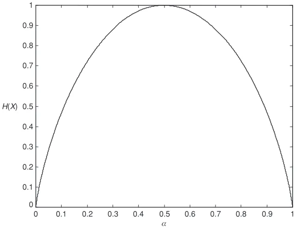
[image:37.432.56.362.54.289.2]α H(X)
Figure 1.4 Entropy function for the binary source
In the above inequality, equality occurs when log21Pi
=log2(M),which means that Pi =
1M.
The maximum value of the entropy is then log2(M), and occurs when all the symbols transmitted by a given source are equally likely. Uniform distribution corresponds to maximum entropy.
In the case of a binary source (M=2) and assuming that the probabilities of the symbols are the values
P0=α P1=1−α (14)
the entropy is equal to
H (X )=(α)=αlog2
1 α
+(1−α) log2
1 1−α
(15)
This expression is depicted in Figure 1.4.
The maximum value of this function is given whenα=1−α, that is,α=1/2,so that the entropy is equal to H (X )=log22=1 bps. (This is the same as saying one bit per binary digit or binary symbol.)
Whenα→1,entropy tends to zero. The function(α) will be used to represent the entropy of the binary source, evaluated using logarithms to base 2.
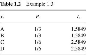
Table 1.2 Example 1.3
xi Pi Ii
A 1/3 1.5849
B 1/3 1.5849
C 1/6 2.5849
D 1/6 2.5849
The entropy is evaluated as
H (X )=2×1
3×log2(3)+2× 1
6×log2(6)=1.9183 bits per symbol
And this value is close to the maximum possible value, which is log2(4)=2 bits per symbol. The information rate is equal to
R=r H (X )=(3000)1.9183=5754.9 bps
1.3 Extended DMSs
In certain circumstances it is useful to consider information as grouped into blocks of symbols. This is generally done in binary format. For a memoryless source that takes values in the range{x1,x2, . . . ,xM}, and where Piis the probability that the symbol xiis emitted, the order
n extension of the range of a source has Mn symbols {y1,y2, . . . ,yMn}. The symbol yi is
constituted from a sequence of n symbols xi j. The probability P(Y =yi) is the probability of
the corresponding sequence xi1,xi2, . . . ,xin:
P(Y =yi)=Pi1,Pi2, . . . ,Pin (16)
where yiis the symbol of the extended source that corresponds to the sequence xi1,xi2, . . . ,xin.
Then
H (Xn)=
y=xn
P(yi) log2
1 P(yi)
(17)
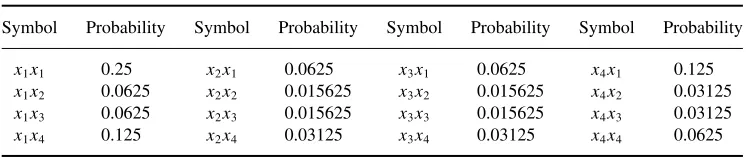
Example 1.4: Construct the order 2 extension of the source of Example 1.1, and calculate its entropy.
Symbols of the original source are characterized by the probabilities P(X =x1)=
1/2,P(X=x2)=P(X =x3)=1/8 and P(X =x4)=1/4.
Symbol probabilities for the desired order 2 extended source are given in Table 1.3. The entropy of this extended source is equal to
H (X2)= M
2
i=1
Pilog2
1 Pi
=0.25 log2(4)+2×0.125 log2(8)+5×0.0625 log2(16)
Table 1.3 Symbols of the order 2 extended source and their probabilities for Example 1.4
Symbol Probability Symbol Probability Symbol Probability Symbol Probability
x1x1 0.25 x2x1 0.0625 x3x1 0.0625 x4x1 0.125 x1x2 0.0625 x2x2 0.015625 x3x2 0.015625 x4x2 0.03125 x1x3 0.0625 x2x3 0.015625 x3x3 0.015625 x4x3 0.03125 x1x4 0.125 x2x4 0.03125 x3x4 0.03125 x4x4 0.0625
As seen in this example, the order 2 extended source has an entropy which is twice that of the entropy of the original, non-extended source. It can be shown that the order n extension of a DMS fits the condition H (Xn)=n H (X ).
1.4 Channels and Mutual Information
1.4.1 Information Transmission over Discrete Channels
A quantitative measure of source information has been introduced in the above sections. Now the transmission of that information through a given channel will be considered. This will provide a quantitative measure of the information received after its transmission through that channel. Here attention is on the transmission of the information, rather than on its generation. A channel is always a medium through which the information being transmitted can suffer from the effect of noise, which produces errors, that is, changes of the values initially transmit-ted. In this sense there will be a probability that a given transmitted symbol is converted into another symbol. From this point of view the channel is considered as unreliable. The Shannon channel coding theorem gives the conditions for achieving reliable transmission through an unreliable channel, as stated previously.
1.4.2 Information Channels
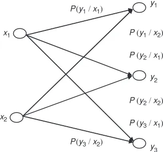
Definition 1.1: An information channel is characterized by an input range of symbols
{x1,x2, . . . ,xU}, an output range {y1,y2, . . . ,yV} and a set of conditional probabilities
P(yj/xi) that determines the relationship between the input xi and the output yj. This
con-ditional probability corresponds to that of receiving symbol yj if symbol xi was previously
transmitted, as shown in Figure 1.5.
The set of probabilities P(yj/xi) is arranged into a matrix Pchthat characterizes completely
the corresponding discrete channel:
x1
y1
y2
y3 x2
P(y3/ x2) P(y1/ x1)
P (y1/ x2)
P (y2/ x1)
P (y2/ x2)
[image:40.432.142.303.55.205.2]P (y3/ x1)
Figure 1.5 A discrete transmission channel
Pch =
⎡ ⎢ ⎢ ⎢ ⎢ ⎣
P(y1/x1) P(y2/x1) · · · P(yV/x1)
P(y1/x2) P(y2/x2) · · · P(yV/x2)
..
. ... ...
P(y1/xU) P(y2/xU) · · · P(yV/xU) ⎤ ⎥ ⎥ ⎥ ⎥
⎦ (18)
Pch =
⎡ ⎢ ⎢ ⎢ ⎢ ⎣
P11 P12 · · · P1V
P21 P22 · · · P2V
..
. ... ...
PU 1 PU 2 · · · PU V ⎤ ⎥ ⎥ ⎥ ⎥
⎦ (19)
Each row in this matrix corresponds to an input, and each column corresponds to an output. Addition of all the values of a row is equal to one. This is because after transmitting a symbol xi, there must be a received symbol yjat the channel output.
Therefore,
V
j=1
Pi j =1, i =1,2, . . . ,U (20)
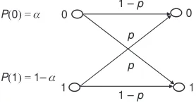
Example 1.5: The binary symmetric channel (BSC).
The BSC is characterized by a probability p that one of the binary symbols converts into the other one (see Figure 1.6). Each binary symbol has, on the other hand, a probability of being transmitted. The probabilities of a 0 or a 1 being transmitted areαand 1−αrespectively.
According to the notation used,
0
p
p
1
0
1 1 – p
1 – p P(0) = α
[image:41.432.140.279.56.129.2]P(1) = 1–α
Figure 1.6 Binary symmetric channel
The probability matrix for the BSC is equal to
Pch=
1−p p
p 1−p
(21)
Example 1.6: The binary erasure channel (BEC).
In its most basic form, the transmission of binary information involves sending two different waveforms to identify the symbols ‘0’ and ‘1’. At the receiver, normally an optimum detection operation is used to decide whether the waveform received, affected by filtering and noise in the channel, corresponds to a ‘0’ or a ‘1’. This operation, often called matched filter detection, can sometimes give an indecisive result. If confidence in the received symbol is not high, it may be preferable to indicate a doubtful result by means of an erasure symbol. Correction of the erasure symbols is then normally carried out by other means in another part of the system. In other scenarios the transmitted information is coded, which makes it possible to detect if there are errors in a bit or packet of information. In these cases it is also possible to apply the concept of data erasures. This is used, for example, in the concatenated coding system of the compact disc, where on receipt of the information the first decoder detects errors and marks or erases a group of symbols, thus enabling the correction of these symbols in the second decoder. Another example of the erasure channel arises during the transmission of packets over the Internet. If errors are detected in a received packet, then they can be erased, and the erasures corrected by means of retransmission protocols (normally involving the use of a parallel feedback channel).
The use of erasures modifies the BSC model, giving rise to the BEC, as shown in Figure 1.7. For this channel, 0≤ p≤1 / 2, where p is the erasure probability, and the channel model has two inputs and three outputs. When the received values are unreliable, or if blocks are detected
p p 0
1
0
1 1− p
1− p
? P (0) = α
P (1) = 1− α x1
x2
y1
y2
y3
[image:41.432.123.300.485.586.2]to contain errors, then erasures are declared, indicated by the symbol ‘?’. The probability matrix of the BEC is the following:
Pch=
1−p p 0
0 p 1−p
(22)
1.5 Channel Probability Relationships
As stated above, the probability matrix Pch characterizes a channel. This matrix is of order
U×V for a channel with U input symbols and V output symbols. Input symbols are char-acterized by the set of probabilities{P(x1),P(x2), . . . ,P(xU)}, whereas output symbols are
characterized by the set of probabilities{P(y1),P(y2), . . . ,P(yV)}.
Pch=
⎡ ⎢ ⎢ ⎢ ⎣
P11 P12 · · · P1V
P21 P22 · · · P2V
..
. ... ...
PU 1 PU 2 PU V ⎤ ⎥ ⎥ ⎥ ⎦
The relationships between input and output probabilities are the following: The symbol y1
can be received in U different ways. In fact this symbol can be received with probability P11if
symbol x1was actually transmitted, with probability P21if symbol x2was actually transmitted,
and so on.
Any of the U input symbols can be converted by the channel into the output symbol y1.
The probability of the reception of symbol y1,P(y1), is calculated as P(y1)=P11P(x1)+
P21P(x2)+ · · · +PU 1P(xU). Calculation of the probabilities of the output symbols leads to
the following system of equations:
P11P(x1)+P21P(x2)+ · · · +PU 1P(xU)=P(y1)
P12P(x1)+P22P(x2)+ · · · +PU 2P(xU)=P(y2)
.. . P1VP(x1)+P2VP(x2)+ · · · +PU VP(xU)=P(yV)
(23)
Output symbol probabilities are calculated as a function of the input symbol probabilities P(xi) and the conditional probabilities P(yj/xi). It is however to be noted that knowledge of
the output probabilities P(yj) and the conditional probabilities P(yj/xi) provides solutions
for values of P(xi) that are not unique. This is because there are many input probability
distributions that give the same output distribution.
Application of the Bayes rule to the conditional probabilities P(yj/xi) allows us to determine
the conditional probability of a given input xiafter receiving a given output yj:
P(xi/yj)=
P(yj/xi)P(xi)
P(yj)
1/4
1 0
7/8 1/8 3/4
0
1
X Y
P (0) = 4/5
[image:43.432.129.291.57.151.2]P (1) = 1/5
Figure 1.8 Example 1.7
By combining this expression with expression (23), equation (24) can be written as
P(xi/yj)=
P(yj/xi)P(xi)
U
i=1P(yj/xi)P(xi)
(25)
Conditional probabilities P(yj/xi) are usually called forward probabilities, and conditional
probabilities P(xi/yj) are known as backward probabilities. The numerator in the above
ex-pression describes the probability of the joint event:
P(xi,yj)=P(yj/xi)P(xi)= P(xi/yj)P(yj) (26)
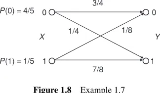
Example 1.7: Consider the binary channel for which the input range and output range are in both cases equal to{0,1}. The corresponding transition probability matrix is in this case equal to
Pch=
3/4 1/4 1/8 7/8
Figure 1.8 represents this binary channel.
Source probabilities provide the statistical information about the input symbols. In this case it happens that P(X=0)=4/5 and P(X =1)=1/5. According to the transition probability matrix for this case,
P(Y =0/X =0)=3/4 P(Y =1/X =0)=1/4 P(Y =0/X =1)=1/8 P(Y =1/X =1)=7/8 These values can be used to calculate the output symbol probabilities:
P(Y =0)= P(Y=0/X =0)P(X =0)+P(Y =0/X =1)P(X =1)
= 3
4× 4 5 +
1 8×
1 5 =
25 40
P(Y =1)= P(Y=1/X =0)P(X =0)+P(Y =1/X =1)P(X =1)
= 1
4× 4 5 +
7 8×
1 5 =
These values can be used to evaluate the backward conditional probabilities:
P(X=0/Y =0)= P(Y =0/X=0)P(X =0)
P(Y =0) =
(3/4)(4/5) (25/40) =
24 25 P(X=0/Y =1)= P(Y =1/X=0)P(X =0)
P(Y =1) =
(1/4)(4/5) (15/40) =
8 15 P(X=1/Y =1)= P(Y =1/X=1)P(X =1)
P(Y =1) =
(7/8)(1/5) (15/40) =
7 15 P(X=1/Y =0)= P(Y =0/X=1)P(X =1)
P(Y =0) =
(1/8)(1/5) (25/40) =
1 25
1.6 The A Priori and A Posteriori Entropies
The probability of occurrence of a given output symbol yjis P(yj), calculated using expression
(23). However, if the actual transmitted symbol xi is known, then the related conditional
probability of the output symbol becomes P(yj/xi). In the same way, the probability of a
given input symbol, initially P(xi), can also be refined if the actual output is known. Thus,
if the received symbol yj appears at the output of the channel, then the related input symbol
conditional probability becomes P(xi/yj).
The probability P(xi) is known as the a priori probability; that is, it is the probability that
characterizes the input symbol before the presence of any output symbol is known. Normally, this probability is equal to the probability that the input symbol has of being emitted by the source (the source symbol probability). The probability P(xi/yj) is an estimate of the symbol
xi after knowing that a given symbol yj appeared at the channel output, and is called the a
posteriori probability.
As has been defined, the source entropy is an average calculated over the information of a set of symbols for a given source:
H (X )=
i
P(xi) log2
1 P(xi)
This definition corresponds to the a priori entropy. The a posteriori entropy is given by the following expression:
H (X/yj)=
i
P(xi/yj) log2
1 P(xi/yj)
i =1,2, . . . ,U (27)
Example 1.8: Determine the a priori and a posteriori entropies for the channel of Example 1.7.
The a priori entropy is equal to
H (X )= 4 5log2
5 4
+1