Primality Testing is Polynomial time: A Mechanised Verification of the AKS Algorithm

(1)

Primality Testing is Polynomial-time:

A Mechanised Verification of the AKS

Algorithm

Hing Lun Chan

A thesis submitted for the degree of

Doctor of Philosophy in Computer Science at

The Australian National University

(2)

(3)

I declare that this thesis is entirely my own work. Although it contains materials from my published work with my supervisor, to the best of my knowledge it does not contain any materials previously published or written by another person except where otherwise indicated.

(4)

(5)

(6)

(7)

Acknowledgments

The completion of this PhD project fulfills my personal dream. It is an achievement built upon extensive help from people all around. Looking back, it took about eight years to finish, and I have been offered every assistance along the way. The list to say thanks is long, but I shall start with my family.

First and foremost, I express my heartfelt thanks to my wife Jantsen. As a mature student, I have my fair share of health issues, family issues, and other age-related issues. She is always the one showing her support with care and patience. I feel confident and comfortable in her presence. She is my angel, and this thesis is dedicated to her.

Without the patient guidance of Michael Norrish, my chief supervisor, this work could not have seen the light at the end of the tunnel. He offers critical advice, accurate judgements, and friendly support. He can tolerate my mistakes, always revealing a way forward when I get stuck. We met regularly on a fortnightly basis to discuss the work progress. The fond memories of each session will last for a lifetime.

Besides being a friend, Michael is also the maintainer of the HOL4 theorem prover. He can guide my skills to take full advantage of the system, and answer all my technical queries with ease. The continual improvement of the HOL4 system is much appreciated, as new features streamline the conversion of proof ideas into scripts. Such convenience in a theorem proving environment deserves many thanks.

I would like to express my gratitude to Peter Baumgartner and Jeremy Dawson, my faithful supervisors, and my superiors Rajeev Gore, Dirk Pattinson, Ranald Clouston and Alwen Tiu. They all show great interest in my work. Peter and Jeremy were keen to enquire about my progress. Rajeev enjoyed my talks and invited me to give guest lectures in his course. Dirk provided me with valuable feedback, Ranald offered opportunities for me to share my work to a wide audience, and Alwen gave me encouragement.

The Australian National University is an excellent institution for intellectual work. I have been given unconditional help from the higher degree research unit, with both administrative support and research training. Many thanks to Elspeth Davies for assisting with my overseas travels, Inger Mewburn for giving valuable advice on my Visualise Your Thesis competition, Candida Spence for kindly providing feedback about my presentation content, and Marie-Claire Miliˇcevi´c for resolving many issues related to my higher degree study.

My thanks extend to Yiming Xu, an ANU undergraduate student doing her research project using my libraries on groups and subgroups. Her excellent work, completed within the short allocated time, shows the general applicability of the libraries I have developed.

Thanks to the many editors of the Journal of Automated Reasoning (JAR), including Jasmin

(8)

Also thanks to Candida Spence of the Information Literacy team at the ANU Library for checking the formatting of this thesis. Numerous errors had been pointed out by anonymous examiners in detailed comments; they have been corrected. The readability of this thesis has been greatly improved by various people, including my wife, Michael Norrish, Jeremy Dawson, and other anonymous reviewers. I am responsible for any remaining mistakes.

Throughout my work, I learn from the masters. I would like to thank those who pointed me in the right direction. John Harrison showed me how to formulate the AKS Main Theorem. Terence Tao clarified by email a difficult point in his AKS webpage. Laurent Théry was fascinated by one of my conference talks that, by the next day, he showed me his scripts reproducing what I had talked about the day before.

Thanks to the AKS team for providing the topic of my research, and bringing to the world such ground-breaking insight into primality testing. I am deeply impressed with the Gödel Prize lecture by Manindra Agrawal, and his many talks sketching the history of the AKS algorithm.

Thanks also to the various authors who offer me well-written textbooks or articles on algebra, especially finite fields, some with lucid expositions of the AKS algorithm. The ideas for the proofs in this thesis are taken from various sources. They are acknowledged in a footnote at the start of the proof, to enhance readability.

Lastly, I would like to thank the world of mathematics, populated by many highly gifted mathematicians. I read broadly, and learn many excellent ideas and techniques through their work. That world is a world of dreams, with wonderful colors one cannot see, and delightful music one cannot hear. The experience is aptly expressed in the following quote:

In the broad light of day mathematicians check their equations and their proofs, leaving no stone unturned in their search for rigour. But, at night, under the full moon, they dream, they float among the stars and wonder at the miracle of the heavens. They are inspired. Without dreams there is no art, no mathematics, no life. — Michael Atiyah1

(9)

Abstract

We present a formalisation of the Agrawal-Kayal-Saxena (AKS) algorithm, a deterministic polynomial-time primality test. This algorithm was first announced by the AKS team in 2002, later improved in 2004. Our work is based on the improved version, with Parts 1 and 2 aim at a formal proof of the correctness of the algorithm, and Part 3 aims at a formal analysis of the complexity of the algorithm. The entire work is carried out in the HOL4 theorem prover.

The correctness of the AKS algorithm relies on a main theorem developed by the AKS team, based on the theory of finite fields. To achieve the goal for Parts 1 and 2, we start by building up a hierarchy of HOL4 libraries for algebraic structures: from monoids, to groups, then rings and fields. Equipped with this foundation, we develop an abstract algebra library cov-ering subgroups, quotient groups, ideals, and vector spaces. We extend the algebra library with polynomials, quotient rings, quotient fields, and finite fields. With all these we can formulate the AKS main theorem, which gives the correctness of the algorithm. For the formal proof, we need to dive into several advanced topics in finite field, in particular the existence and uniqueness of finite fields, and properties of cyclotomic polynomials.

Although algebraic structures, including finite fields, have been formalised in other theorem provers, our work is the first such comprehensive library in HOL4, covering also the uniqueness of finite fields up to isomorphism. Furthermore, by casting the AKS main theorem in the context of finite fields, we can see clearly the inter-relationship of various parts of the proof. As a result, we can make slight adjustments to the published version of the AKS algorithm. These slight adjustments are minor in terms of the significance of the AKS achievement, answering the challenge "Is Primes in P?" in the affirmative, but they simplify the implementation and analysis of the AKS algorithm.

The AKS algorithm consists of several loops: loops for checking if a condition still holds, and loops for searching if a condition will hold. Thus for the goal of Part 3, we embark on an analysis of such loops: formalising their behaviour, in particular the bound on the number of iterations. The AKS algorithm mostly involves modular computations, using numbers or manipulating polynomials. We develop tools and techniques to formally assert the recurrence properties of loop computations, with emphasis on the analysis of the time complexity behaviour. As far as we know, this approach to complexity analysis has not been done in other theorem provers.

Many offshoots from this work are interesting, even new to published proofs of the AKS algorithm. We have an elegant proof to a key result that enables us to slightly improve the bound on the AKS parameter. We present the relationship between the AKS algorithm and the AKS main theorem. We distill a picture to visualise the logic behind the proof of the AKS main theorem. We show in detail an implementation of the AKS algorithm that is suitable for loop analysis of complexity. We introduce an approach to study the time complexity of simple loops.

(10)

(11)

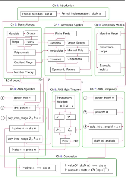
List of Figures

1.1 Dependency Diagram of thesis topics. Terms and symbols are defined in the relevant chapters. Very briefly, hereFLTis Fermat’s Little Theorem, andPHPis

the Pigeonhole Principle. . . 10

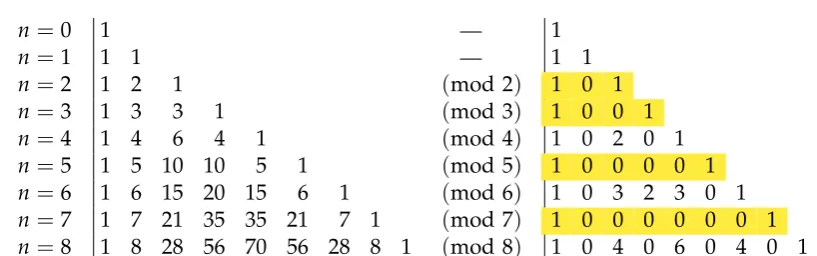
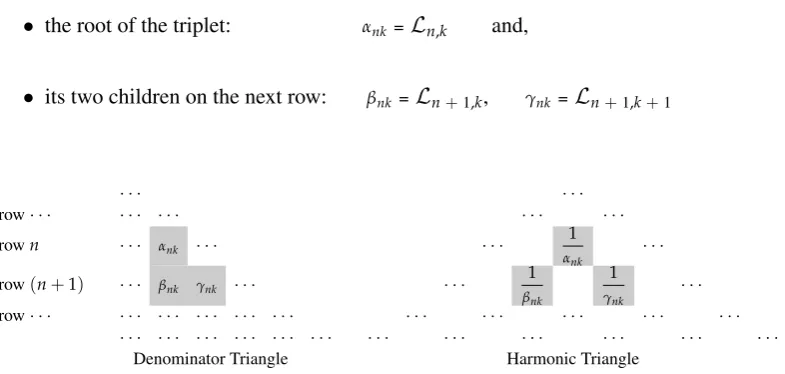
2.1 Pascal’s Triangles: the one on the left shows the binomial coefficients, the one on the right has each row depicting the remainders under division by the corre-sponding row index. The colored rows, with remainders in-between all equal to zero, have row indexes that areprime. . . 28

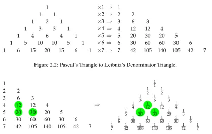
2.2 Pascal’s Triangle to Leibniz’s Denominator Triangle. . . 32

2.3 Leibniz’s Denominator Triangle and Harmonic Triangle. . . 32

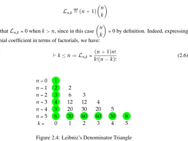
2.4 Leibniz’s Denominator Triangle . . . 33

2.5 The Leibniz triplet: in Denominator Triangle and in Harmonic Triangle. . . 34

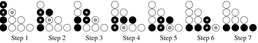
2.6 Transformation of a path from vertical to horizontal in the Denominator Trian-gle, stepping from left to right. The path is indicated by entries with black discs. The 3 gray-dotted discs in L-shape indicate the Leibniz triplet, which allows LCM exchange. Each step preserves the overall LCM of the path. Hence the black discs of Step 1 and of Step 7 have the same LCM. . . 36

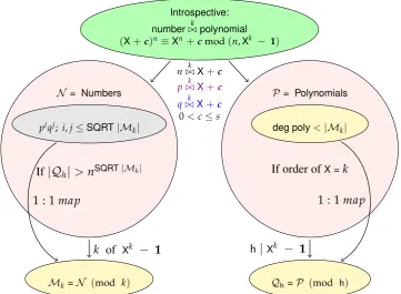
5.1 Sketch of the AKS proof. The introspective relations ofnand p, a prime divi-sor ofn, together with the cofactor q = n div p, give rise to two setsN andP (Section 5.3). By taking modulo ofk andh, an irreducible factor ofXk − 1, respectively, the setsN andP map, correspondingly, to two finite setsM_k and Qh(Section 5.4). Two finite subsets ofN andPcan be crafted such that injec-tive maps between finite sets can be constructed, as illustrated, if the parameters kandsare suitably chosen to satisfy the “if” conditions (Section 5.5 and Sec-tion 5.6). Once these “if” condiSec-tions are established, ifnis not a perfect power of p, the grey set will have more than|M_k|elements. This is impossible as the injective map on the left will contradict the Pigeonhole Principle (Section 5.7). Thereforenmust be a perfect power of its prime divisorp. . . 80

7.1 Polynomial as a list of cofficients, with the least significant coefficient on the left. 121 7.2 Polynomial introspective check: p=qinR_n_,_k =Z_n[X]/(Xk − 1). . . 122

8.1 Dependency Diagram of Section 1.6, page 10. . . 132

(16)

(17)

List of Tables

1.1 Phases of the AKS algorithm.. . . 3

3.1 Selected values of the AKS parameter byaks_paramn. . . 48

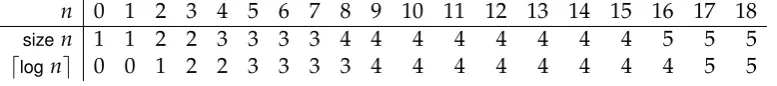
6.1 Comparison of measuressizenanddlogne. . . 97

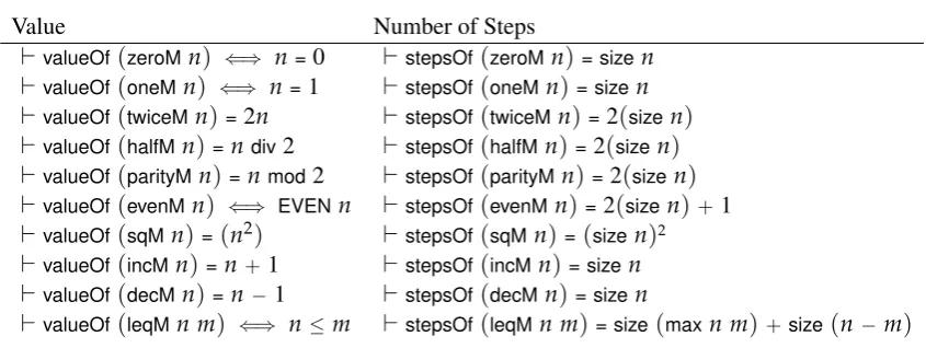
6.2 Subroutines values and number of steps. . . 100

6.3 Types of Recurrence Loop . . . 105

7.1 Steps to perform introspective computations for unnormalisedX+c. . . 121

(18)

(19)

List of Algorithms

1 The AKS algorithm in pseudo-code . . . 44 2 The algorithm in AKS revised paper, Agrawal et al. [2004]. . . 44

(20)

(21)

Publications

Parts of this thesis have been published as the papers listed below. Some ideas in Chapter 3 and Chapter5, on the correctness of the AKS algorithm, first appear in the second paper. Some parts of Chapter2on basic algebra come from the first and third papers. Chapter4on advanced algebra is based on the fourth paper.

Hing Lun Chan and Michael Norrish. A String of Pearls: Proofs of Fermat’s Little Theorem. In Chris Hawblitzel and Dale Miller, editors, Proceedings of Certified Pro-grams and Proofs, 2012. LNCS number 7679, pages 188—207. Springer, December 2012. Print ISBN: 978-3-642-35307-9, doi: 10.1007/978-3-642-35308-6_16. Also pub-lished in Andrea Asperti, editor,Journal of Formalized Reasoning. Volume 6, number 1, pages 63—87. December 2013. ISSN 1972-5787, doi: 10.6092/issn.1972-5787/3728.

Hing Lun Chan and Michael Norrish. Mechanisation of AKS Algorithm: Part 1 — the Main Theorem. In Christian Urban and Xingyuan Zhang, editors, Interactive Theorem Proving, ITP 2015. 6th International Conference, Nanjing, China, August 24-27, 2015, Proceedings. LNCS number 9236, pages 117—136. Springer, August 2015. First Online 19 August 2015, doi: 10.1007/978-3-319-22102-1_8.

Hing Lun Chan and Michael Norrish. Proof Pearl: Bounding Least Common Multiples with Triangles. In Jasmin Christian Blanchette and Stephan Merz, editors, Interactive Theorem Proving, ITP 2016. 7th International Conference, Nancy, France, August 22-25, 2016, Proceedings. LNCS number 9807, pages 140—150. Springer, August 2016. First Online 07 August 2016, doi: 10.1007/978-3-319-43144-4_9. Also published in Jour-nal of Automated Reasoning, Springer Netherlands. First online 14 October 2017, doi: 10.1007/s10817-017-9438-0. Printed in February 2019, Volume 62, Issue 2, pages 171— 192.

Hing Lun Chan and Michael Norrish. Classification of Finite Fields with Applications. InJournal of Automated Reasoning, Springer Netherlands. First online 25 October 2018, doi: 10.1007/s10817-018-9485-1. Printed in October 2019, Volume 63, Issue 3, pages 667—693.

(22)

(23)

Chapter1

Introduction

This thesis is about a formal proof of the Agrawal-Kayal-Saxena (AKS) algorithm in the theorem-prover HOL4. This is based on a formal definition of the AKS algorithm, with a proof of its correctness. This is followed by a formal implementation of the AKS algorithm, with a proof of its computational complexity based on a machine model. We identify 3phases for the AKS algorithm, highlighting the role of a critical parameter k, and its effect on performance. We touch on the impact of the AKS algorithm, and why its formalisation is significant. We discuss what has been done, what we have achieved, and the layout of this thesis.

If you can’t explain your mathematics to a machine, it is an illusion to think you can explain it to a student. — Nicolaas Govert de Bruijn (2003)1

1 .

1 Formalisation

To formalise is to understand, in detail: explain the logic to a machine, as de Bruijn proclaims. There are many levels to understand a mathematical proof. Take the example of the AKS algorithm, the theme topic of this thesis. The AKS team presented their proof in nine pages (Agrawal et al. [2002, 2004]). Expositions of various lengths and depths have been written (Bernstein [2002]; Aaronson [2003]; Saptharishi [2007]), whole chapters have been devoted to this topic (Crandall and Pomerance [2005]; Shoup [2008]; Rempe-Gillen and Waldecker [2014]), even a whole book (Dietzfelbinger[2004]) has been published. Nonetheless, to the Fields medalistTerence Tao[2009], the essence of the proof can be understood within a single webpage.

A formalisation, with proof scripts to be compiled by a theorem-prover, provides yet another level of understanding, one that is machine-checkable. The formalisation process reveals the dependency of various concepts, identifies their intricate relationships, and ultimately unfolds the logical threads that lead to the validity of the result.

For the formalisation of the AKS algorithm, we are keen to understand:

1_{From his invited lecture titled}_{Memories of the Automath Project. For a delightful discussion of this quote, see}_Zen and the art of formalizationbyAsperti and Avigad[2011].

(24)

1. What is the AKS algorithm?

2. Is the AKS algorithm correct?

3. How to implement the AKS algorithm?

4. What is the run-time behaviour of the AKS algorithm?

The AKS algorithm is about primes, a major topic in number theory. The first involves some concepts in modular arithmetic, using numbers and polynomials. The second involves some knowledge of abstract algebra, in particular the theory of finite fields. The third involves an appreciation of machine execution, with some understanding of subroutines. The fourth involves a model to execute an algorithm, and techniques to solve recurrence relations.

Our formalisation therefore touches on a potpourri of topics in mathematics. However, all topics lead back to the AKS algorithm. For a peek at these topics, see Figure1.1.

1 .

2 PRIMES is in P

Given a numbern greater than1, a primality test is a method to determine if n isprime, i.e., whethernhas only the trivial factors1and itself.2

The primality test takes the form of an algorithm: a step-by-step method with inputnand output the verdict: nis prime or not. The run-time behaviour of an algorithm is an estimate of the number of steps from input to output. Intuitively, the larger the input number, the more the number of steps. To formalise this idea, we need at least a notion of the input size.

It is customary to measure the size of inputnby(log n), the base2logarithm ofn, which is indicative of its number of binary digits. Throughout this work, we shall use insteaddlogne, the round-up value, which is defined3 for all values ofn. An algorithm with input n and its number of steps bounded by a polynomial function ofdlog nebelongs to class P, the class of polynomial-time algorithms. Compare to the class of exponential-time algorithms, such class P algorithms are considered efficient, at least in theory.

The name PRIMES refers to the class of primality test algorithms. Since internet security protocols make use of primes with many digits to generate keys, an efficient primality test is keenly sought after. For a long time, only probabilistic primality tests in class P are known, but deterministic primality tests are theoretically more desirable. A deterministic and efficient primality test remains elusive, and the challenge to find one is known as “Is PRIMES in P?”.

On August 4, 2002, the AKS team announced their algorithm in a paper (Agrawal et al. [2002]) with the title “PRIMES is in P”. This immediately caused a sensation throughout the computer science community, even making news headlines in the popular press.4 After careful analysis by experts, the AKS algorithm was substantially refined inAgrawal et al.[2004]. The

2_{Note that}₀_{is never a prime, and}₁_{is a unit, neither prime nor composite.} 3_{We define}_d_log_0e₌_{0, while}_log_{0 is undefined.}

(25)

§1.3 AKS Phases 3

breakthrough was officially recognized when the AKS team was awarded the Gödel Prize by the European Association for Theoretical Computer ScienceEATCS[2006]:

The result obtained by Agrawal, Kayal, and Saxena can be seen as a crowning achievement of a long algorithmic and mathematical quest.

A remarkable aspect of the article is that the final exposition itself turns out to be rather simple. The text as published in Annals of Mathematics is a masterpiece in mathematical reasoning. It has a high density of tricks and techniques, but the arguments come in a brilliantly simple manner; they remain completely elementary. The contents of the paper are therefore accessible to a broad audience.

The revised version shows that the AKS algorithm can determine whether a numbern is prime with the number of steps bounded by some polynomial function ofdlogne152. The rather

high polynomial exponent means the AKS algorithm cannot compete with the known proba-blilistic primality tests.

Nevertheless, the AKS algorithm remains the only known unconditional, deterministic and polynomial-time primality test. We shall refer to the first2002paper as theoriginalAKS paper, and the later2004paper as therevisedAKS paper, or simply the AKS paper.

1 .

3 AKS Phases

The AKS algorithm consists of3phases:

AKS Algorithm

Input:a numbern

Output:decide whethernisPRIME

Phase 1 Power Free Test the numbernis not a square, not a cube,etc.

ifnis not power free,nis notPRIME

Phase 2 Parameter Search the parameterkis chosen with some criteria based onn

ifkis a factor ofn,nisPRIMEonly whenk=n

Phase 3 Polynomial Checks identities to hold under two moduli involvingnandk. ifnpasses all polynomial identity checks,nisPRIME

Table 1.1: Phases of the AKS algorithm.

Phase 1 is a preliminary step. This is because the theory behind the AKS algorithm, to be presented in Parts I and II, shall declare that, if the input npasses the checks of Phase3from a good parameter k of Phase2, then n = pe for some prime pand exponent e. With Phase 1

ensuring thatnis power free, the exponente=1. Therefore,nis prime.

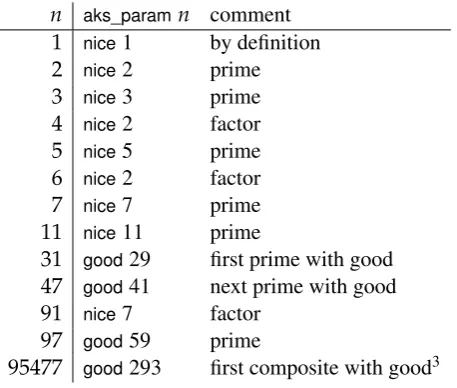
For Phases2and3, Table1.1shows the appearance of a parameterk. As we shall see, this AKS parameterkis central to the AKS algorithm. Its existence through a search comprises the whole of Phase 2. The search, denoted byaks_param n, is sequential. The search can give3

(26)

1. anicek, wherekis a factor ofn,

2. agoodk, wherekis not a factor ofn, and satisfies a special condition,

3. abadsituation, where the search, up to some cut-off, fails to find anicekor agoodk.

We shall spell out details of the search (Section3.3.1), and prove that the search never fails. If Phase2returns a parameter of the typenice k,kis a factor ofn. Thereforenis prime if and only if this factor is itself,i.e., n= k. On the other hand, if a parameter of the typegood k

is returned, this parameterk is used to drive Phase3, which consists of a series of polynomial identity checks of the form:

(X + c)n ≡ Xn + c(mod n, Xk − 1) (1.1)

for a range of constants c, i.e., 0 < c ≤ s. The limit s is specified by an expression based on n andk. Details of such polynomial identity checks will be explained later, but the form of the polynomial identity is so striking that the AKS team suggested a special term for this form: anintrospectivecheck. We shall eventually see how such introspective polynomial checks characterise the AKS algorithm.

With these notions, we can get a glimpse of our formal definition of the AKS algorithm:

Definition 1. The AKS algorithm with3phases.

aksndef=

power_freen∧

caseaks_paramnof | nicek . k=n

| goodk.

∀c.0<c∧c≤(SQRT ϕ(k))dlogne⇒(X + c)n ≡ Xn + c(mod n, Xk − 1) | bad . F

Note how our formal definition ofaksntakes into account the3phases of the AKS algorithm. We shall formally establish that the AKS algorithm, backed up by some beautiful results from the theory finite fields, stands up to its claim:

Theorem 2. The AKS algorithm is a primality test.

`primen ⇐⇒ aksn

(27)

§1.4 AKS Formalisation 5

Definition 3. The AKS algorithm implemented in monadic style.

aksMndef

=

do

b ← power_freeMn;

ifbthen do

c ← paramMn;

casecof

| nicek . eqMk n

| goodk . poly_intro_rangeMn k k

| bad . returnF

od

else returnF

od

and prove these important results, where valueOf (aksM n)is the final value of the monadic computation with inputn, andstepsOf ◦ aksMis the number of steps of monadic computation expressed as a function ofn:

Theorem 4. The AKS implementation is correct, and belongs to the polynomial class.

`valueOf(aksMn) ⇐⇒ aksn

`stepsOf◦aksM∈O(dlogne21)

These results constitute our formal proof of the AKS algorithm,i.e., “PRIMES is in P”. Given that our implementation of the AKS algorithm is not intended for efficiency, and our model of elementary computations is quite conservative (see Section6.3), together with the fact that our recurrence theory vastly over-estimates for the sake of simplicity, we are happy with our O(dlogne21). The original AKS paper estimated the algorithm5in the orderO(de logne12), and

the revised AKS paper lowered this toO(de logne

15 2).

1 .

4 AKS Formalisation

Because the AKS algorithm is a major milestone in primality testing, we would like to formally verify the authors’ claim, to be100%confident of the breakthrough.

The AKS algorithm depends critically on a parameterk derived from the input number n. In the original AKS paper, the parameter kneeds to be a prime, and its bound depends on the Prime Number Theorem for the distribution of primes, and the Brun-Titchmarsh Theorem for an upper bound on the distribution of primes in an arithmetic progression. Using these results

5_The e

(28)

from analytic number theory, the AKS team obtained an upper bound for parameterk, showing that the AKS algorithm is in P, the class of polynomial-time algorithms.

The Prime Number Theorem aims at the limiting behaviour of the distribution of primes. However, if only the bounds on the distribution is required, such a result had been obtained by Chebyshev. This result is known as a weak form of the Prime Number Theorem.

When experts examined the AKS proof, they realized that while the best bound for the parameter k depends on those theorems of analytic number theory, the weak form of prime distribution can already produce an acceptable bound, still keeping “PRIMES is in P”. Therefore, initial attempts to formalise the AKS algorithm concentrated on establishing prime distributions of some form in theorem provers. As early as 19 August 2002, JohnHarrison[2002] mentioned during his talk on formalisation of real numbers that:

By the way, some deep results about the distribution of primes are used in the recent polynomial-time primality-testing algorithm. . .

As reported inWiedijk[2003], John Harrison formalised, in HOL Light, a weak form of the Prime Number Theorem and a theory of cyclotomic polynomials for this purpose.

Laurent Théry [2003] discussed the formalisation of algorithms in number theory: those related to primes and primality tests. He reported a formal proof of the Miller-Rabin algorithm, a probabilistic primality test, by Joe Hurd [2003]. He predicted that the next candidate for formalisation will be the AKS algorithm.

Théry observed that there is no relationship between the description of an algorithm and the difficulty of its formal proof. As an example in the report, he found that a correctness proof in Coq of the simple Knuth’s algorithm to list the firstnprimes required a variety of techniques, including a formal proof of Bertrand’s postulate.6 This was prior to the revised AKS paper, thus he was concerned that a formal proof of the AKS algorithm will involve much deeper properties about primes than Bertrand’s postulate.

With the role of the Prime Number Theorem in determining the bound on the parameterk

clarified, the proof in the revised AKS paper of2004 is considered “simple and elementary”, as expressed in the Gödel Prize2006citation (see Section1.2). The improvements concern the parameterk:

• The parameterkis no longer required to be prime. Instead, the correctness proof of the AKS algorithm is obtained by invoking properties of cyclotomic polynomials, which is a standard topic in finite field theory.

• Since the condition onkis relaxed, the bound on its size no longer depends explicitly on Prime Number Theorem. Instead, the bound can be derived from a lemma about a lower bound on the least common multiple of consecutive numbers. The lemma has a standard proof by elementary calculus in the literature.

These improvements cleaned up the presentation of the AKS algorithm.

(29)

§1.5 Our Contribution 7

Due to these simplications, there was renewed interest to formalise the AKS algorithm. Indeed,Campos et al.[2004] tried in ACL2, andde Moura and Tadeu[2008] attempted in Coq. Both only showed that a prime will pass all the AKS tests. This is the easy part. The hard part is show that a non-prime cannot pass all the AKS tests.

1 .

5 Our Contribution

Our goal is to achieve a formal proof of “PRIMES is in P”, based on the AKS algorithm. This includes a proof of its correctness, both the easy and hard parts, and a proof of its complexity, establishing that the AKS algorithm is indeed in the polynomial-time class.

We aim for a formalisation in HOL4 that is:7

• self-contained, not relying on external libraries of previous work,

• elementary, not involving concepts from analysis of real-valued functions, and

• algebraic, following the improved version of the algorithm by the AKS team.

Our work in the formalisation of the AKS algorithm is built up by layers. We develop theories for various topics, many of these are interesting by themselves.

In a previous effort, we formalised the correctness of the AKS algorithm, both the easy and hard parts, in Chan and Norrish [2015]. In that work, we followed the original AKS paper, taking the parameterkto be a prime. We also establishedk’s existence on general grounds, but without giving it a bound.

In this thesis, we follow the revised AKS paper, and achieve the following:

1. We prove a lemma about a lower bound on the least common multiple of consecutive numbers without any use of calculus. Instead, the lemma is established by an ingenious use of the Leibniz’s triangle, a variant of the Pascal’s triangle. The lower bound given by the lemma provides a bound on the parameterkof the AKS algorithm (Definition1).

2. The correctness of the AKS algorithm (Theorem2) is now proved with parameter k no longer required to be prime. This is a result of another effort, the formalisation of finite field theory including cyclotomic polynomials.

3. We have a formal implementation of the AKS algorithm (Definition3), involving details of each phase. The implementation is not optimized for performance, but it simplifies the subsequent complexity analysis.

4. We reach the ultimate goal: a proven correct implementation of the AKS algorithm, with verification that its computational complexity is indeed bounded by a polynomial of the input size (Theorem4).

(30)

5. Our work is backed up by a thorough formalisation of finite fields, from the hierarchy of algebraic structures, to their existence and uniqueness up to isomorphism by cardinality. The collection of abstract algebra libraries is developed with generic types. It has proved its usefulness in several key areas in the formalisation of AKS algorithm.

6. We introduce a simple monadic framework to analyse the computational complexity of algorithms. This proves to be adequate to show that the AKS algorithm runs in polynomial time.

Thus we achieve a complete formal elementary proof of the correctness of the AKS algorithm, and provide an elementary complexity analysis to verify “PRIMES is in P”.

Our theorem prover is HOL4, and our techniques are allelementary: basic number theory, and standard abstract algebra. We build a fairly complete library for finite fields, including quotient fields, cyclotomic polynomials, culminating in their existence and uniqueness for the classification of finite fields.

1 .

6 Thesis Structure

In order to present a coherent account of the formalisation of the AKS algorithm, with minimal distraction from other issues, this thesis is structured into chapters, as follow:

1. Introduction — an overview of the AKS formalisation work (Chapter1).

2. Part 1: Foundation

• Basic Algebra — number theory and algebra theorems (Chapter2).

• AKS Algorithm — a study of its phases and parameters (Chapter3).

3. Part 2: Correctness

• Advanced Algebra — finite field and cyclotomic factors (Chapter4).

• AKS Main Theorem — a formal proof of the correctness of algorithm (Chapter5).

4. Part 3: Complexity

• Complexity Models — toolkit for computational complexity analysis (Chapter6).

• AKS Complexity — implemetation and analysis of the algorithm (Chapter7).

5. Conclusion — summary and preview of future work (Chapter8).

(31)

§1.7 Summary 9

HOL4 Sources Our entire respository of HOL4 proof scripts can be found at this location: http://bitbucket.org/jhlchan/hol/src/. The respository is tagged withphd-thesis-02, and consists of sub-foldersaks/,/algebraand/algorithm. Each folder or subfolder has a description of its content in a file namedREADME.md. Scripts in the repository are provided in two formats:

• those with suffix.holare intended for use in interactive HOL4 sessions,

• those with suffixScript.smlare intended for HOL4 compilation usingHolmakefile.8

We shall omit the suffix when referring to proof scripts. Each proof script has documentation in block comments at the beginning. The full library of proof scripts is described in Appendix (SectionA.2, page152). Hyperlinks have been set up for each Definition, Theorem, Lemma, and Corollary to associate with the actual location of the item in our repository.

1 .

7 Summary

We introduce the AKS algorithm through its3phases, and formulate our goals: to prove that it is a primality test (Theorem2), and to show that an implementation is correct and has a run-time bounded by a polynomial function of the input size (Theorem4). Together they verify formally that the AKS algorithm exemplifies “PRIMES is in P”. The revised AKS paper, complete with traditional proofs of both the correctness and complexity of the AKS algorithm, consists of only nine pages. Although the paper is short, there is a substantial amount of coding to be done in order to formalise the AKS algorithm from the ground up. Most of the work relates to the proper development of the supporting libraries. Our discussion shall be divided into 3 Parts: Foundation, Correctness, and Complexity. We start with Part 1, to develop a blueprint for the formalisation work.

1 .

8 Remarks

For informative accounts of formalisation of mathematics and automated theorem proving, see JohnHarrison [1996] and his talks over the years (Harrison[2013, 2015]). A comprehensive survey of iteractive theorem proving was given by Andrea Asperti [2009]. An article titled

Formally Verified Mathematicswas contributed by JeremyAvigad and Harrison[2014]. Another recent talk on advances of formal mathematics was given by JosefUrban[2016].

During December 2008, the Notices of the American Mathematical Society (Magid[2008]) publishedA Special Issue on Formal Proof. In August 2011, the journal Mathematical Structures in Computer Science (Curien[2011]) had a special issue onInteractive Theorem Proving and the Formalisation of Mathematics. In February 2013, the Journal of Automated Reasoning had

Special Issue: Formal Mathematics for Mathematicians(Trybulec et al.[2013]).

(32)

Formal definition: aksn Formal implementation: aksMn Monoids Groups Rings Fields Polynomials Quotient Rings Number Theory Finite Fields

Subfields Vector Spaces

Irreducibles Minimal Poly.

Existence Uniqueness Cyclotomic Factors Machine Model Recurrence Loops Example: logMn power_freen aks_paramn

poly_intro_rangeZ_nk n s

`primen⇒aksn

poly_intro_rangeZ_p k n s

`aksn⇒primen

Introspective Relation:

n./k X+c

N P

M_k Qh

Proof

power_freeMn

paramMn

poly_intro_rangeMn k s

aksMn: analysis

`primen ⇐⇒ aksn `valueOf(aksMn) ⇐⇒ aksn

`stepsOf◦aksM∈O(dlogne21)

Ch1: Introduction

Ch2: Basic Algebra

Ch3: AKS Algorithm

Ch4: Advanced Algebra

Ch5: AKS Main Theorem

Ch6: Complexity Models

Ch7: AKS Complexity

[image:32.595.109.528.90.680.2]

Ch8: Conclusion k p FLT LCM bound h 1 1 2 2 3 3 PHP

(33)

§1.9 Notation 11

1 .

9 Notation

All statements starting with a turnstile (`) are HOL4 theorems, automatically pretty-printed to LA_{TEX from the relevant theory in the HOL4 development. Generally, our notation allows an} appealing combination of quantifiers (∀,∃), logical connectives (∧for “and”,∨for “or”,¬ for “not”,⇒ for “implies”, and ⇐⇒ for “if and only if”), with logical constantsT for true, and

F for false. For functional notation, we use λ for function abstraction, and juxtaposition for function application.

Set-theoretic Notation We use standard set notations: ∈ for set membership, ∪ for set union,∩for set intersection, and set comprehensions such as{x | x<7}. The universal set of typeαis denoted byU(:α). For a finite setS, the cardinality is written|S|, the sum over its

elements is

∑

S, and the product over its elements is

∏

S.

List Notation Lists are enclosed in square-brackets[ ], with list members separated by semi-colon (;), using infix operators :: for “cons”, _for append, and . .for inclusive range. When `=h::t,his the head of`andtis the tail of`. The empty list is[ ]. For a nonempty list`,LAST` picks the element at the end, and FRONT `takes all elements except the end. Other common list operators are: LENGTH,SUM,REVERSE, andMEM for list member. We useλ for function abstraction, and juxtaposition for function application. The application of a single argument function f to every elementxin a listxsis denoted byMAP f xs. Extending this to a function of two arguments,MAP2 f xs ysdenotes the application of f taking the first argument fromxs

and the second argument fromys.

Relation and Maps Given a binary relationR, its reflexive and transitive closure is marked by an asterisk (∗),i.e.,R∗. We write f : s ,→ tto mean that function f is injective from sets

to sett, and write f : s ↔ tto mean that function f is bijective from setsto sett.

Multiplication Except for explicit products like 7× 13=91, we shall use juxtaposition for the product of two numbersxandy, asxy. When a function fis applied to a product, it is shown as f xy; whereas(f x)yshows the product of f x andy. This convention closely resembles the traditional presentation in mathematics. In other domains, e.g., algebraic structures and polynomials, we shall usex×yto represent the product of two elementsx,y.

(34)

ROOT k nis the integerk-th root ofn, SQRT nis the integer square root of n, n div 2 is the integer half ofn, anddlogneis the round-up of the logarithm ofnin base2.

HOL4types The HOL4 theorem prover uses a simple type system. Our formalisation of the AKS algorithm uses the basic number type,num, and sets and lists derived from number type. In order for abstract algebra to be applicable to objects of various types, the algebraic structures are defined over a generic typeα.

(35)

Part I

Foundations

Part 1 is about the AKS algorithm, from pseudocode to primality test. For each phase of the algorithm, we define concepts to formalise the actions, and develop theories with background from basic algebra. Showing a prime can go through the AKS algorithm is straight-forward. Proving a number going through the AKS algorithm must be a prime needs a strategy: get a prime, build a finite field, and formulate the AKS Main Theorem in finite field. The AKS Main Theorem is the focus of Part 2, but all preparatory work are provided in Part 1.

(36)

(37)

Chapter2

Basic Algebra

This chapter walks through various topics in algebra that are basic for an understanding of the AKS algorithm. We describe our formalisation of abstract algebra, from monoids and groups, to rings and fields. The correctness proof of the AKS algorithm draws ideas from the theory of finite fields. Modular systems, based on numbers and polynomials, provide examples of these algebraic structures. Their properties and terminology are frequently used in discussions of the AKS algorithm. We begin with fairly obvious definitions and results, but finish with some remarkable formulae, including a novel approach to the first lemma in the AKS paper.

Mathematics is the work of the human mind, which is destined to study rather than to know, to seek the truth rather than to find it. — Évariste Galois (1832)1

2 .

1 Algebraic Structures

It was the work of Galois’ mind where the concept of a group was first conceived and studied. This transformed the study of algebra: from concrete numbers to abstract structures. Moreover, a short paper byGalois[1830] laid the foundation for the study of finite fields — they are also called Galois fields in his honour.

The theory behind the AKS algorithm is based on finite fields. Our formalisation of finite fields is at the top of a hierarchy of theories defining a family of algebraic structures:

• AMonoidMwith a binary operation×that is closed, associative, and has an identity#e. An abelian monoid,AbelianMonoidM, has the operation also commutative.

• AGroupGis a monoid with an inversex−1_{for each element}_x_{such that}_x_× _x−1₌_{#e. An} abelian group,AbelianGroupG, is a commutative group.

• A commutative Ring R has two components, a group R.sum with operation + and a monoidR.prodwith operation×. Both share the same carrier, and:

1_{From his writing}_{On the progress in pure analysis, as translated in}_Neumann_[₂₀₁₃_].

(38)

◦ R.sumis an abelian group with identity0;

◦ R.prodis an abelian monoid with identity1;

◦ Multiplication is distributive over addition.

• AFieldF is a commutative ring, with all nonzero elements having multiplicative inverses;

i.e., they form a groupF∗.

Our formalisation takes only the commutative ring, since our target is the finite field. Hereafter, rings are understood to be commutative rings. This hierarchy exemplifies the naïve approach to algebra in HOL4, which is sufficient for the purpose of this thesis.

The traditional mathematical presentation and notations undergo some drastic modifications when rendered in HOL. We first determine our representation for these algebraic structures. At our base, we have theαmonoidtype:

αmonoid=h[carrier:α → bool; op:α → α → α; id:α]i

A monoid(M : α monoid)is a value of the α monoidtype, effectively a triple of three different fields. Using the HOL record machinery, we can refer to these fields with a pleasant “dot” notation; e.g., M.op. The M.carrier is a subset of all possible values of type α; the operation M.op is a binary operation on those values and the identityM.id is one of those values.

It is then straightforward to define the predicateMonoidover such values that carves out those that satisfy the axioms of a monoid. Here we annotate the definition’s variables with their types, and remove the special overloading used in the rest of this thesis so that uses of M.op are explicit.

Definition 5. Axioms of a monoid: closure, associativity and identity.

Monoid(M :αmonoid)def

=

(∀(x:α) (y:α).x∈M.carrier∧y∈M.carrier⇒M.opx y∈M.carrier)∧ (∀(x:α) (y:α) (z:α).

x∈M.carrier∧y∈M.carrier∧z∈M.carrier⇒

M.op(M.opx y)z=M.opx(M.opy z))∧ M.id ∈M.carrier∧ ∀(x:α).x∈ M.carrier⇒M.opM.idx=x∧M.opxM.id =x

A group G is a monoid with all its elements invertible. By hiding the underlying types, and overloadingG.carrier by G, G.op x y by x × y, and G.id by #e, the result is better for readability:

Definition 6. A group is a monoid with every element having an inverse.

(39)

§2.1 Algebraic Structures 17

We can prove that such inverses are unique and are inverses on the left and right. Skolemizing, we define the inverse function, and characterise it thus

` GroupG ⇒ ∀x.x∈G⇒x×x−1₌_#e_∧_x−1 _×_x₌_#e

The ring type consists of a combination of two monoid values:

αring= h[carrier :α → bool; sum:αmonoid; prod:αmonoid]i

For a ringR, its additive monoid is denoted byR.sumand its multiplicative monoid is denoted byR.prod. When we come to define the ring axioms, we can use prettier syntax in the description of the distributive law. In other words, x + y is really R.sum.op x y, and x × y is really R.prod.opx y. Denoting the carrier of ringRbyR, this is the definition of a ring in HOL4:

Definition 7. Axioms of a ring: additive group, multiplicative monoid, and distribution law.

RingRdef=

AbelianGroupR.sum∧AbelianMonoidR.prod∧R.sum.carrier = R∧R.prod.carrier = R∧

∀x y z.x∈R∧y∈R∧z∈R⇒x×(y+z)=x×y+x×z

Finally, the definition of what it is to be a fieldF can be quite terse:

Definition 8. A field is a ring with nonzeros forming a multiplicative group.

FieldF def=RingF ∧GroupF∗

HOL4Conventions In HOL4, definitions such as these subsequently require that all theorem statements to be qualified with assumptions such as Field F. This is because the valueF is just a pair of record values, and is not known to satisfy the field axioms without that explicit assumption. Though tedious, these qualifications of our theorem statements do not significantly impact the theorem-proving task. Rather, the burden lies mostly in the initial writing of the goal. Although overloading can be used to pretty-print for readability, we keep the types barely visible through the use of different fonts. For example, a fieldF has elements in the carrierF, with the nonzero elementsF∗forming a groupF∗.

In the rest of this thesis, overloading is used extensively to hide complicated terms such as R.sum.op x y, but the logical assumptions (such asField F) always appear. Occasionally, this can make the assumption seem vacuous as the syntax for the operators no longer appears to refer back to the value (e.g.,F) at all. For example, this apparent vacuousness can be seen in the last ring axiom above.

(40)

2 .

2 Monoids and Groups

Both monoid and group have only one operation, generally called multiplication. Repeated multiplication of an elementxby itselfntimes is exponentiation, with the usual notationxn. By definition,x0₌_{#e. It may happen that}_xn ₌_#e_{for some}_n_>₀_{. The smallest such exponent}_n_is

the multiplicative order ofx, or simply theorderofx, denoted byorder_M(x):

Definition 9. The multiplicativeorder_M(x)is the least nonzero exponent to give the identity, or zero is no such exponent exists.

0<n⇒(order_M(x)=n ⇐⇒ xn=#e∧ ∀m.0<m∧ m<n⇒xm6=#e)

order_M(x)=0 ⇐⇒ ∀n.0<n⇒xn 6=#e

Although findingxn=#edoes not imply thatnis the order, we do have:

Theorem 10. The order of a monoid element divides an exponent that can give the identity.

` MonoidM⇒ ∀x n.x∈M⇒(xn=#e ⇐⇒ order_M(x)|n)

Proof. Letk = order_M(x). Dividing n by k gives a quotient q and a remainderr, such that

n=qk +randr<k. Thus,

#e=xn=xqk+r=xk ×xr=#ek ×xr=xr

Thereforexr =#e. Butr <kand orderkis minimal, sor=0. In other words,k |n.

This enables us to deduce the order ofxnfrom the order ofx:

Theorem 11. For a monoid element, the order of its power is reduced by the greatest common divisor of the power and its order.

`MonoidM⇒ ∀x n.x∈M∧0<n⇒order_M(xn)= order_M(x)div gcd(n,order_M(x))

Proof. Letk= order_M(x),y=xn,j= order_M(y), andd= gcd(n,k). Sinced|nandd|k„

ykdivd=(xn)kdivd=(xk)ndivd=#endivd=#e

Thusj|kdivdby order divides exponent (Theorem10).

Withj|kdivdandkdivd|j,j=kdivd.

We writeH≤Gto mean thatHis a subgroup ofG:

(41)

§2.2 Monoids and Groups 19

Definition 12. A subgroupHof groupGis a group with subset carrier and the same operation.

H≤Gdef

=Group H∧GroupG ∧H⊆G ∧H.op =G.op

Similar ideas apply to submonoids. A subgroup can also be identified by:

Theorem 13. LetH be a nonempty subset of the groupG equipped with the group operation. If for all elementsx,y∈ H,x×y−1 _∈_H_{, then}_H_{is a subgroup of}_G_.

` H≤G ⇐⇒

GroupG ∧H.op =G.op∧H.id =G.id∧H6=∅∧H⊆G∧ ∀x y.x∈H∧y∈H⇒G.opx(y−1₎_∈ _H

Since a subgroupHinduces an equal-size partitionviacosets, we have:

Theorem 14. (Lagrange’s Theorem). For a finite groupG, the cardinality of any subgroup is a divisor of|G|.

` H≤G ∧FINITE G⇒|H|||G|

For a finite group G, there are only a finite number of elements. Let a ∈ G. Then the set {a,a2,a3, . . .}is finite. Together with the group operation, this forms a subgroup, called the group generated by elementa, denoted byhai. Its cardinality is easily derived:

Theorem 15. For an element a with nonzero order in a finite groupG, the subgrouphaihas cardinalityorder_G(a).

`GroupG ∧ a∈G∧0<order_G(a)⇒|hai.carrier|= order_G(a)

Applying Lagrange’s Theorem (Theorem14), we have:

Theorem 16. In a finite groupG, the order of an element divides|G|.

` FiniteGroupG ⇒ ∀a.a∈G⇒order_G(a)||G|

We can also derive this important result:

Theorem 17. In a finite group, an element raised to cardinality exponent gives the identity.

`FiniteGroupG ∧ a∈G⇒a|G| =#e

Proof. Let elementain a finite groupG has orderk. Thenak =#e. Now|G|is a multiple ofk,

i.e.,|G|=qkfor someq. Thusa|G| ₌₍_ak₎q₌_#eq₌_#e.

Order Notation Although the order of an element xin a monoidMshould be denoted by

(42)

order ofkin the monoidZ∗_n.3 Later in Section4.2, we shall introduce quotient rings over rings Ror fieldsF, and writeorder_h(X)for the order of polynomialXin the monoidR∗

h[X]orFh∗[X] derived from a modulus polynomialh.

2 .

3 Rings and Fields

A ring with1 = 0is called a trivial ring. A field is a non-trivial ring, since1 is inF∗ with 0 excluded. As noted in Section2.1, our rings are more commonly known as commutative rings with identity. We did not go all the way to non-commutative rings since our goal is about finite fields. By the same token, we do not consider skew fields. However, we do consider other algebraic structures related to fields,e.g., integral domains in Section2.4.

Letabe a nonzero element in a ring. Due to the distributive law, and the fact that1×a=a, all nonzeroahave the same additive order as1. The unique additive order of1in a ringR is called itscharacteristic, denoted bychar(R):

Definition 18. The characteristic of a ring is the additive order of its multiplicative identity.

char(R)def=order_R_._sum(1)

The characteristic of a finite ring is positive: the smallest number of repeated additions of 1 giving0.

The multiplicative invertibles of a ringRare called units, denoted byR∗_{. Since each unit} has a multiplicative inverse, we have:

Theorem 19. The units of a ring form a group.

` RingR⇒GroupR∗

For a fieldF, all nonzero elements are units, by definition, and the group isF∗.

2 .

4 Integral Domains

Since a fieldF has a multiplicative groupF∗, it means that the product of two nonzero elements cannot be0, by multiplicative closure. Hence a field has no zero divisors, an instance of a special kind of ring:

Definition 20. An integral domain is a non-trivial ring with no zero divisors.

IntegralDomainDdef=

RingD∧ 16=0∧ ∀x y.x∈D∧y∈D⇒(x×y=0 ⇐⇒ x=0∨y=0)

3_For_k_{not in the monoid}_Z∗

(43)

§2.5 Polynomials 21

For an integral domainD, letabe a nonzero element,i.e.,a6=0. If the integral domain is finite, the sequencea,a2_,_a3_{, . . .} _{must repeat. Suppose}_aj ₌ _aj+k _{for some} _j_and_k _with_k ₆₌ _{0. Then}

ring subtraction and distribution give aj × (ak − 1) = 0. The absence of zero divisors in an integral domain implies thatak =1. Note thatak =1andk6=0 means thatahas a multiplicative inverse: ak−1_{. Therefore:}

Theorem 21. A finite integral domain is always a field, hence a finite field.

`FiniteIntegralDomainF ⇒FieldF

`FiniteIntegralDomainF ⇒FiniteFieldF

This allows us to conclude that a finite non-trivial ring is a finite field simply by checking that there are no zero divisors (see Section4.2, page61).

2 .

5 Polynomials

Polynomials are expressions of the form:

cnXn+cn−1Xn−1+· · ·+c1X+c0 (2.1)

where the coefficients cj come from a ring R. These polynomials, equipped with the usual

polynomial addition and multiplication, form a polynomial ring, denoted by R[X]. In these polynomial rings, the additive identity is0, the zero polynomial, and the multiplicative identity is 1, the constant polynomial one. When the ring R has further properties,e.g., without zero divisors so that it is an integral domainD, or all nonzero elements are invertible so that it is a fieldF, we shall denote the polynomial ring byD[X]orF[X], respectively.

Polynomial Implementation For simplicity, polynomials are implemented as finite lists. Indeed, our type (α poly) is a synonym for (α list) in HOL4. Internally, a polynomial of type α is a list of cofficients taken from U(:α), with the first element the constant term, and the last element the leading coefficient. The zero polynomial0is taken as the empty list, its degree is defined as 0, and the degree of a nonzero polynomial is defined as one less than its length. The results of polynomial operations are normalised, so that a nonzero polynomial always has a nonzero leading coefficient. Polynomial addition is componentwise list addition, and polynomial scalar multiplication is componentwise list scaling. Polynomial multiplication is defined by list recursion, using addition and scalar multiplication. Polynomial division requires proper notions of a polynomial divisor and a polynomial remainder, see Section2.5.1. Further discussion of our implementation is deferred to Section8.2.2,Polynomial as lists(page135).

Polynomial Notation Denote byhthe polynomial as given in (2.1). For this polynomialh, its degree isdeg h=nand its leading coefficient isleadh=cn. If all coefficients are zero, then

(44)

A polynomialh with coefficients from a ring R, as in (2.1), can be viewed as a function inX. The valuation h(a) is the value of h when X is substituted by an element a ∈ R. We extend the notion of substitution to polynomials: substituting theXin polynomialhby another polynomialggives a polynomialh_Jg_K.4 We also extend the modulus notation for polynomials,

e.g.,f ≡ g (mod h)means that bothf andggive the same remainder after division byh. In other words,h

|

(f −g).

2.5.1 Polynomial Modulus

For polynomial division, the polynomial divisorhis called the modulus. Besides requiring the modulus to be nonzero,h 6= 0, there are other restrictions for the modulush. We first consider the general case, where the polynomials have coefficients from a ringR.

Clearly, a monic modulus can always perform the long division for any polynomial dividend — since a suitable multiple of the modulus can cancel the leading term of the dividend. Thus the degree of the dividendpis reduced at each step, leading to termination of the division process with this result:

p=pdivh ×h+pmodh (2.2)

where(pdivh)is the quotient, and(pmodh)is the remainder. When the modulus is not monic, this division process is possible only when the leading coefficient of the modulus is invertible,

i.e., a unit element in a ring, denoted by unit (lead h). In this case, both the dividend and the modulus can be multiplied by the inverse of the leading coefficient of the modulus, reducing the polynomial division to the monic situation.5

For polynomial division to terminate with(p divh)and(p mod h)satisfying Equation2.2, the degree of the remainder has to be strictly less than the degree of the modulus. This means 0 <deg h,i.e., the modulus is not a constant polynomial. In this case, polynomial division by modulushsatisfies:

` RingR∧polyp∧polyh∧unit(leadh)∧0<degh⇒

p=pdivh×h+pmodh∧deg (pmodh)<degh

When the modulushis a constant polynomial, we have:

`RingR ∧polyp∧polyh ∧unit(leadh)∧degh=0⇒pdivh=(leadh)−1_×_p

`RingR ∧polyp∧polyh ∧unit(leadh)∧degh=0⇒pmodh=0

We lose the fact that the degree of the remainder decreases, but retain the Euclidean Equation2.2. Thus in our formulation, division of polynomials with coefficients from a ringRis defined only for certain types of modulus: those polynomials with leading coefficient invertible. Since nonzero field elements are invertible, any nonzero polynomial with coefficients from a fieldF can be a modulus.

4_{Viewing polynomials as functions, this is their function composition.}

(45)

§2.5 Polynomials 23

In this thesis, many theorems concerning polynomial division with coefficients from a ring are presented with the version of a monic modulus, though a more general version of the theorem may also have been proved. This is adequate because, when applied to the AKS algorithm, the modulus isXk − 1withk>0, which is monic, or one of its monic factorsh.

2.5.2 Polynomial Divisibility

An irreducible polynomial, denoted byipoly p, has only trivial factors. Letzbe an irreducible polynomial. If the irreduciblezdivides a power, sayz | pn, it must divide the base,i.e.,z | p. Extending this result to a setSof monic irreducible polynomials, denoted bymisetS, and write

∏Sfor the product of all polynomials in the setS, we have:

Theorem 22. For polynomials with coefficients from a field, letq=∏ Sbe a product of monic irreducibles. Ifqdivides a polynomial power, thenqdivides the polynomial base.

`FieldF ∧FINITES∧ misetS∧polyp∧pn ≡ 0(mod ∏S)⇒p ≡ 0(mod ∏S)

This result is used in the proof of Theorem 102, regarding an exponent for the introspective relation.

2.5.3 Polynomial Roots

An elementais a root of polynomialhifh(a)=0. The roots of polynomialhis the setrootsh, orroots_Rhif the underlying ringRneeds to be specified. Each rootagives a factor(X− a):

Theorem 23. (Root Factor Theorem). Each polynomial root corresponds to a linear factor dividing the polynomial.

`RingR⇒ ∀ha.polyh∧a∈R⇒(h(a)=0 ⇐⇒ (X−a)|h)

If the coefficients of a polynomial are from a field, the leading coefficient can always be reduced to1by multiplying with its inverse. This shows that such a polynomial will have the same roots as the resulting monic polynomial.

Although a polynomial with coefficients from a ring may have more roots than its degree6, this cannot happen when its coefficients come from a ring without zero divisors,i.e.,

Lemma 24. A nonzero polynomial with coefficients from an integral domain has no more roots than its degree.

`IntegralDomainF ⇒ ∀h.polyh∧h6=0⇒|rootsh|≤degh

Since a field is also an integral domain, this result holds for polynomials with coefficients from a field:

6_{For example, in}_Z_6,₂_∗₃₌_{0. Hence in}_Z

(46)

Theorem 25. A nonzero polynomial with coefficients from a field cannot have more roots than its degree.

`FieldF ⇒ ∀p.polyp∧ p6=0⇒|rootsp|≤degp

Thus a polynomial with coefficients from a field with positive degreenhas at mostnfactors.

2 .

6 Finite Fields

The characteristic of a finite field is particularly interesting:

Theorem 26. A finite field has prime characteristic.

`FiniteFieldF ⇒prime char(F)

Proof. A field has no zero divisors, thus its characteristic has no proper factor.

2.6.1 Field Orders

A finite fieldF is an integral domain, with all nonzero elements inF∗ having nonzero orders. The set of elements with order equal tonis denoted by(orders F∗ n). Its cardinality is related to the Euler’sϕ-function,ϕ(n), counting the number of coprimes from1ton:

Theorem 27. In a finite fieldF, the number of elements with ordernisϕ(n)ifndivides|F∗|, otherwise0.

`FiniteFieldF ⇒ ∀n.|ordersF∗ n|=ifn||F∗|then ϕ(n)else0

Proof. 7In a finite fieldF, the multiplicative groupF∗_{is finite. Let}_q₌_|_F∗_{|, then every element} has a nonzero order that dividesq(Theorem16). Thusorders F∗ 0= ∅, and|orders F∗ 0|=0. Forn>0, first observe that field elements of the same order are in power form of each other:

`FiniteFieldF ⇒ ∀x y.x∈F∧y∈F∧order_F∗(x)= order_F∗(y)⇒ ∃j.y=xj

This is because both elements are roots ofXk − 1, where kis their common order. Let zbe an field element of orderk, then z,z2, . . . ,zk are all roots of Xk − 1, which can have at most

k roots (Theorem25). Thusz is a generator of the multiplicative cyclic group of the roots of

Xk − 1, denoted by(GeneratedF∗ _z_):

`FiniteFieldF ⇒ ∀z.z∈F∧z6=0⇒roots(XorderF∗(z)₋₁₎₌₍_Generated_F∗ _z₎_._carrier

Moreover, the order of a power (Theorem11) for a field element is:

`FieldF ⇒ ∀x.x∈F⇒ ∀n.0<n⇒order_F∗(xn)= order_F∗(x)div gcd(n,order_F∗(x))

(47)

§2.6 Finite Fields 25

This means that if orders F∗ _n _{is nonempty with an element} _x_{, the elements in the set are} precisely thosexk_where_k_{is coprime to}_n_{. Thus}_|_orders_F∗ _n_|₌ _ϕ(_n_{), the count of coprimes to}

nnot exceedingn.

We claim thatordersF∗ _n_{is nonempty whenever}_n_| _q_{. Suppose the contrary, that}_n_| _q_but

ordersF∗ _n₌_∅_{. Let}_u₌_divisors_q_,_v₌ _{_d_∈_divisors_q_|_orders_F∗ _d₆₌_∅_{}. Then}_n_∈_/_v_{, so that}

vis a proper subset ofu. Therefore, byv⊂u,

∑

d∈v

ϕ(d)<

∑

d∈u

ϕ(d)

Note that every field element has an order that dividesq, and the setsordersF∗ _d_{for various} divisor d ofq form a partition ofF∗. Since each value d ∈ v has|orders F∗ d| = ϕ(d), the

left-hand side is:

∑

d∈v

ϕ(d)=

∑

d∈v

|ordersF∗ d|= [

d∈v

ordersF∗ d

=|F∗|=q

and using an identity for Euler’s ϕ-function, the right-hand side is:

∑

d∈u

ϕ(d)=

∑

d|q

ϕ(d)=q by Theorem58near the end.

Combining both sides, we haveq< q, a contradiction. HenceordersF∗ n6=∅.

2.6.2 Cyclic Multiplicative Group

This is a fundamental feature about finite fields:

Theorem 28. The multiplicative group of a finite field is cyclic.

` FiniteFieldF ⇒cyclicF∗

Proof. 8By Theorem27, the setordersF∗ _|_F∗_|₆₌_∅_{. Thus there exists a field element of order} |F∗|,i.e., a generator ofF∗, making it cyclic.

2.6.3 Primitives

A generator of the cyclic groupF∗of the finite fieldF is called aprimitiveof the finite field:

Definition 29. A primitive of a finite fieldF is an elementzwith order|F∗|.

z∈ordersF∗ _|_F∗_|def

=z∈F∗ ∧order_F∗(z)=|F∗|

By Theorem27, there areϕ(|F∗|)primitives for a finite fieldF. We shall see the role played by primitives in Section4.3.2about isomorphic fields.

(48)

2 .

7 Number Theory

The abstract concepts of algebraic structures have some concrete applications, one of which concerns the modular systems in our next topic. This is relevant to the AKS algorithm because the introspective checks (see Section1.3, Equation1.1) are polynomial computations with dou-ble moduli (mod n,Xk − 1). We also take this opportunity to walk through some topics in number theory. Some results are well-known, while some are not. They all have a place in understanding the nature of the AKS algorithm.

2.7.1 Modular Systems

Given a modulusn, the remainders under (mod n)form the ringZn:

Theorem 30. For positiven, the ringZ_nhas cardinalitynand characteristicn.

`0<n⇒RingZ_n

` |_Z_n.carrier|=n

`0<n⇒char(Zn)=n

Homomorphism is a structure-preserving map between two algebraic structures of the same type: between monoids, groups, rings, or fields. Here is a homomorphism between two rings, indicated by(7→_r):

Theorem 31. Ifmis a factor ofn, then (mod m)is a homomorphism between the ringsZ_n andZ_m.

`0<n∧m|n⇒(λx.xmodm):Zn7→rZm

Proof. Sincenis a multiple ofm, taking (mod n)then (mod m)is the same as taking (mod m) once. Therefore we have, for twox,yless thann:

(x +y)modnmodm=(x+y)modm=(xmodm+ymodm)modm xymodnmodm=xymodm=(xmodm)(ymodm)modm

Thus the map preserves both modular addition and multiplication, hence a homomorphism.

This result is used later in the proof of introspective shifting (Theorem71, page52).

Given two numbersm,n, their greatest common divisord = gcd(m,n)can be expressed as a linear combination ofmandn, by Bézout’s identity:

`0<m⇒ ∃p q.pm=qn+gcd(m,n)

Ifgcd(m,n)=1, thenmhas a multiplicative inversepin (mod n). Therefore,

Definition 32. The units in the ringZ_nare the elements coprime ton.

Z∗

n

def

=

Primality Testing is Polynomial time: A Mechanised Verification of the AKS Algorithm