Increasing power of robust test through pre-testing in multiple regression model

INCREASING POWER OF ROBUST TEST THROUGH

PRE-TESTING

IN MULTIPLE REGRESSION MODEL

Rossita M Yunus1_{andShahjahan Khan}

Department of Mathematics and Computing, Australian Centre for Sustainable Catchments, University of Southern Queensland, Toowoomba, Q 4350, Australia.

Emails: [email protected], [email protected]

ABSTRACT

In this paper, we define (i) unrestricted (UT), (ii) restricted (RT) and (iii) pre-test (PTT) tests for testing the significance of a subset of the parameters of a multiple regression model when the remaining parameters are (i) completely unspecified, (ii) specified at fixed values or (iii) suspected at fixed values. The M-estimation methodology is used to formulate the three tests. The asymptotic distribution of the test statistics are used to derive the asymptotic power function of the tests. Analytical and graphical comparisons of the three tests are obtained by studying the power functions with respect to the size and power of the tests. The PTT shows a reasonable dominance over the other two tests asymptotically.

KEYWORDS

pre-test, asymptotic distribution, asymptotic power, M-estimation, contiguity, bivariate non-central chi-square.

2000 Mathematics Subject Classification:62G20, 62G35, 62G10

1 Introduction

The multiple regression model is arguably the most commonly used statistical model in many real life problems. In many cases a large number of explanatory variables are in-cluded in the multiple regression model. Not all the explanatory variables contribute

sig-1_{on leave from Institute of Mathematical Sciences, Faculty of Sciences, University of Malaya, Malaysia.}

© 2010 Pakistan Journal of Statistics ₁₅₁

nificantly to the prediction of the response variable. There are several methods available to exclude the non-significant explanatory variables from the model. In the context of testing hypotheses on any arbitrary subset of regression parameters, one may use the non-sample prior information on the explanatory variables to improve the power of the test on the coef-ficients of the remaining explanatory variables. Depending on the type of prior information various tests may be derived. It is important to investigate and compare the properties of the tests in order to select a test with the maximum power.

LetXi,i=1, . . . ,n,benobservable response variables of a multiple regression model,

Xi=β0ci+ei, (1.1)

whereβ0= (β1,β2, . . . ,βp)is a p-dimensional row vector of unknown regression

param-eters,c0

i= (c1i, . . . , cpi)is a p-dimensional row vector of known real constants of the

in-dependent variables,eiis the error term which is identically and independently distributed

symmetric about 0 with a distribution function,Fi, i=1, . . . ,n.The vector ofp-regression

parameters can be expressed asβ0= (β0₁,β0₂)whereβ0₁is a sub-vector of orderrandβ0₂

is a sub-vector of dimensionssuch thatr+s=p. Similarly, partitionc0

ias(c0i1,c0i2)with

c0

i1= (c1i, . . . , cri)andci02= (c(r+1)i, . . . ,cpi).

Consider testing the significance of the sub-vector β₁under three conditions on the values of the sub-vectorβ₂: (i) unspecified (ii) specified and fixed (iii) uncertain. For case (i), we want to testH?

0 :β1=0 againstHA?:β1>0 with test function, φUTn .This test is

called the unrestricted test (UT). For case (ii), the test for testing ofH?

0 :β1=0 against

H?

A:β1>0 with test functionφRTn is called the restricted test (RT). For case (iii), testing

H₀(1):β₂=0 is recommended to remove the uncertainty of the suspicious values ofβ₂=0 before testing the significance ofβ₁. The testing onH₀(1):β₂=0 againstH_A(1):β₂>0 with test functionφPT

n is known as a pre-test (PT). If the null hypothesis of this pre-test is

rejected, the UT is used to testH?

0, otherwise the RT is used. The ultimate test for testing

H?

0 following a pre-testing onH (1)

0 is defined as the pre-test test (PTT) and the test function is denoted byφPT T

n .

Many studies considered the estimation of parameters with non-sample prior informa-tion on the values of the parameters for various models. This includes commonly known preliminary test and Stein-type shrinkage estimators (see for instance, Khan and Saleh, 1997 and 2001, [1, 2]). However, in this paper we pursue the testing problem of the inter-cept parameter under non-sample prior information on the slope parameter. Some studies on the effect of the PT on the power of the PTT are found in literature for parametric cases [3, 4] as well as for the non-parametric cases [5, 6, 7]. Tamura (1965) [5] investigated

the performance of the PTT for one sample and two samples non-parametric problems. Saleh and Sen (1982, 1983) [6, 7] proposed UT, RT and PTT based on rank test for sim-ple linear model and simsim-ple multivariate model in two separate articles. Using sampling distribution theory of rank statistics, they developed the procedures to obtain the power functions for each test. Other than these two regression models, the UT, RT and PTT are also proposed for the parallelism model. As such, Lambert et al. (1985) [8] derived size and power of the UT, RT and PTT using the tests that are based on the least-squares (LS) estimators. Although the tests based on LS estimators do not depend on the assumptions of the underlying distribution of the error term, the LS estimates are identical to the maximum likelihood (ML) estimates when the distribution of the error term is assumed to be normally distributed. Both ML estimates and LS estimates are non robust with respect to deviation from the assumed (normal) distribution (c.f. [9, p.21]). So, it is suspected that the tests based on LS estimators are also non robust. The robust R-estimators are derived from the rank tests because rank tests are asymptotically distribution free under the null hypothesis (c.f. [10, p.281]). However, rank tests often preserve information about the order of the data but discard the actual values, thus overlook information that may have led to a better solution [11]. The most popular robust estimation method, however, is the M-estimation. The M-estimation method is applied to the actual data, hence, its statistical test does not suffer the same kind of lost of information as the rank test. One of the robust tests formu-lated using the M-estimation methodology is the M-test. The M-test is originally proposed by Sen (1982) [12] using the score function in the M-estimation methodology. It is ex-pected that the M-test formulated by the M-estimation procedures inherits the robustness properties of the estimation method, so the test is less sensitive to departures from model assumptions. Sen (1982) [12] introduced the M-test for testing the significance ofβ₂only. Recently, few unpublished papers [13] have used M-test for the UT, RT and PTT in the regression model to investigate the performance of the tests.

statistics; here these results are adopted for a different model in the context of testing after pre-test.

The investigations on the comparisons of the UT, RT and PTT for simple multivariate model [7] and parallelism model [8] are limited to analytical discussion only; the compu-tational comparisons of the UT, RT and PTT are not provided in these papers. Perhaps, the computational comparison of the UT, RT and PTT could not be given due to the nonexis-tence tool to compute the power functions at that time. To compute the power of the PTT, the bivariate integral of the non-central chi-square distribution is required. However, the proposed bivariate non-central chi-square distribution in literature at the time their papers were published are very complicated and not practical for computation. In this paper, we refer to Yunus and Khan (2009b) [15] for the computation of the bivariate integral of the non-central chi-square distribution. For simple multivariate model and parallelism model, according to Saleh and Sen (1983) [7] and Lambert et al. (1985) [8], the power of the PTT may be between those of the UT and RT. However, this statement is not clearly supported by arguments in their papers probably due to the complicated form of the bivariate non-central chi-square distribution that they used in the papers. Although multiple regression model is considered in this paper, we obtain quite similar findings as the simple multi-variate and parallelism models because the test statistic for the PTT is bimulti-variate noncentral chi-square distribution for all of these models. We discussed their statement in the findings of this paper and support our findings with clear arguments and through simulated studies. Along with some preliminary notions, the method of M-estimation is presented in Sec-tion 2. The UT, RT and PTT are defined in SecSec-tion 3. In SecSec-tion 4, the asymptotic distri-bution of the proposed test statistics are derived. These distridistri-butions are used to obtain the power functions of the tests in Section 5. The analytical comparisons of the UT, RT and PTT are also given in Section 5. The comparisons of the power function of the UT, RT and PTT through simulation example are provided in Section 6. The final section presents discussions and concluding remarks.

2 The M-estimation

Given an absolutely continuous functionρ:ℜ→ℜ, M-estimator ofβ is defined as the solution of minimizing the objective function

n

∑

ρ

µ

Xi−β0ci

Sn

¶

with respect toβ∈ℜp.HereSnis an appropriate scale statistic for some functionalS=

S(F)>0. IfFisN(0,σ2_),S

n=MAD/0.6745 is an estimate ofS=σ,whereMADis the

mean absolute deviation ([16, p.78], [17, p.387]). Ifψ=ρ0_{, then the M-estimator ofβis}

the solutions of the system of equations,

n

∑

ciψ

µ

Xi−β0ci

Sn

¶

= 0. (2.2)

For any randsdimensional column vectors, t1 andt2 (r,s∈ℜ), consider the statistics below

Mn1(t1,t2) =

n

∑

ci1ψ µ

Xi−t01ci1−t02ci2

Sn

¶

, (2.3)

Mn2(t1,t2) =

n

∑

ci2ψ µ

Xi−t01ci1−t02ci2

Sn

¶

. (2.4)

For a nondecreasingψ:ℜ→ℜ,let ˜β₂be the constrained M-estimator ofβ₂whenβ₁=0, that is, ˜β₂is the solution ofMn2(0,t2) =0 and it may be conveniently be expressed as

˜

β₂= [sup{t2:Mn2(0,t2)>0} +inf{t2:Mn2(0,t2)<0}]/2 (2.5)

(cf. [12]). Note that for nondecreasingψfunction,Mn2(0,t2)is decreasing ast2is

increas-ing (c.f. [9, p.85]). Similarly, let ˜β₁be the constrained M-estimator ofβ₁whenβ₂=0, that is, ˜β₁is the solution ofMn1(t1,0) =0 and conveniently be expressed as

˜

β₁= [sup{t1:Mn1(t1,0)>0} +inf{t1:Mn1(t1,0)<0}]/2. (2.6)

Theorem 1. Given the asymptotic properties of Mn1(·,·)and Mn2(·,·)in equations (A.1),

(A.2) and (A.3) in the Appendix A, asymptotically,

(i) n−12M_n 1(0,β˜2)

d

→Nr(0,σ20Q1?)under H0?:β1=0, (2.7)

(ii) n−12M_n 2(β˜1,0)

d

→Ns(0,σ20Q2?)under H0(1):β2=0, (2.8)

where Q?

1=Q11−Q12Q−221Q21and Q?2=Q22−Q21Q−111Q12.

Here,Nr(·,·)represents anr-variate normal distribution with appropriate parameters.

Letσ2 0=

R_∞

−∞ψ2 µ

X−β0c

S

¶

dF(X−β0c). Hereσ2

0is the second moment ofψ(·)while the first moment is zero by assumingFis symmetrically distributed at 0 andψis a skew sym-metric function. TakeQ11=limn→∞_n1Qn11=limn→∞

1

n∑ni=1ci1c0i1,Q12=limn→∞1_nQn12=

limn→∞1_n∑in=1ci1c0i2,Q21=limn→∞_n1Qn21=limn→∞

1

3 The UT, RT and PTT

3.1 The unrestricted test (UT)

Ifβ₂is unspecified,φUT_n is the test function ofH₀?:β₁=0 againstH_A?:β₁>0. UnderH₀?,

Xi=β02ci2+ei.We consider test statistic

T_nUT =Mn1(0,β˜2)

0

Q?_n1−1Mn1(0,β˜2)

S(1)n

2 ,

where ˜β₂(given in equation (2.5)) is a constrained M-estimator ofβ₂underH₀?. It follows from equation (2.8) thatTUT

n isχ2r(chi-square distribution withrdegrees of freedom) under

H?

0 asn→∞,withQ?n1 =Qn11−Qn12Q

−1

n22Qn21andS

(1)

n

2

=∑ ψ2

µ

Xi−β˜

0

2ci2

Sn

¶

/n.

Let `UT

n,α1 be the critical value of T

UT

n at the α1 level of significance. So, for the test functionφUT

n =I(TnUT > `UTn,α1), the power function of the UT becomesΠ

UT

n (β1) =

E(φUT

n |β1) =P(TnUT > `UTn,α1|β1),whereI(A)is an indicator function of the setA.It takes

value 1 ifAoccurs, otherwise it is 0.

3.2 The restricted test (RT)

Ifβ₂=0,φRT_n is the test function for testingH₀?:β₁=0 againstH_A?:β₁>0. The proposed test statistic is

T_nRT=Mn1(0,0)

0_Q

n11

−1_M

n1(0,0)

S(2)n

2 .

It follows from equation (A.3) that for largen,TRT

n →d χ2r underH0:β1=0,β2=0 where

Sn(2)

2

=∑ ψ2

³

Xi Sn

´

/n.Again, let`RT_n,α2 be the critical value ofT_nRT at theα2level of sig-nificance. So, for the test functionφRT

n =I(TnRT > `RTn,α2), the power function of the RT

becomesΠRT

n (β1) =E(φRTn |β1) =P(TnRT> `RTn,α2|β1).

3.3 The pre-test (PT)

For the preliminary test on the slope,φPT_n is the test function for testingH₀(1):β₂=0 against

H_A(1):β₂>0. UnderH₀(1),Xi=β01ci1+ei.The proposed test statistic is

TPT

n =

Mn2(β˜1,0)

0

Q?_n2−1Mn2(β˜1,0)

S(3)n

where ˜β₁ (given in equation (2.6)) is a constrained M-estimator of β₁. It follows from equation (2.7) thatTPT

n d

→χ2

s underH0(1), whereQ?n2 =Qn22−Qn21Q

−1

n11Qn12 andS

(3)

n

2

=

∑ ψ2

µ

Xi−β˜

0

1ci1

Sn

¶

/n.

3.4 The pre-test test (PTT)

LetφPT T_n be the test function for testingH₀(1)following a pre-test onβ.Since the PTT is a choice between RT and UT, define,

φPT T_n =I[(T_nPT < `PT<sub>n,α3</sub>,T<sub>n</sub>RT > `RT_n,α2)or(T_nPT > `PT<sub>n,α3</sub>,T<sub>n</sub>UT> `UT_n,α1)], (3.1)

where`PT_n,α3 is the critical value ofT_nPT at theα3level of significance. The power function of the PTT is given by

ΠPT T_n (β₁) =E(φPT T_n |β₁) (3.2)

and the size of the PTT is obtained by substitutingβ₁=0 in equation (3.2).

4 Asymptotic distribution of UT, RT, PT and PTT

In this section, the asymptotic distributions of UT, RT, PT and PTT are derived under local alternative hypotheses,{Kn}(see below). These distributions are essential to obtain the

power functions of the UT, RT and PTT. To derive the power function of the PTT, we require to find the joint distributions of£TUT

n ,TnPT

¤

and£TRT n ,TnPT

¤ .

Theorem 2. Let{Kn}be a sequence of local alternative hypotheses, where

Kn:(β1,β2) = (n−

1

2_λ1,n−12_{λ2), (4.1)}

withλ1=n

1 2β

1>0andλ2=n

1 2β

2>0are (fixed) real numbers. Under{Kn},

asymptoti-cally,

(i) _

 n−

1 2M_n

1(0,β˜2)

n−12M_n 2(β˜1,0)

  d

→Np

 

  γQ?1λ1

γQ? 2λ2

 _,σ2

0 

 Q?1 Q?12

Q? 21 Q?2

  

_{, (4.2)}

(ii)

  n−

1 2M_n

1(0,0)

n−12M_n 2(β˜1,0)

  d

→Np

 



 γ(Q11λ1+Q12λ2)

γQ? 2λ2

 _,σ2

0 

 Q11 0

0 Q?

where Q?₁₂ =Q12Q−221Q21Q−111Q12−Q12, Q21? =Q21Q−111Q12Q22−1Q21−Q21 and γ= 1S

R_∞

−∞ψ0 µ

X−β0c

S

¶

dF(X−β0c).

Theorem 3. Under{Kn}, asymptotically(TnRT,TnPT)are independently distributed as

bi-variate noncentral chi-square distribution with(r,s)degrees of freedom and(TUT n ,TnPT)

are distributed as correlated bivariate noncentral chi-square distribution with(r,s)degrees of freedom and noncentrality parameters,

θUT = γ2 σ2 0

(λ0₁Q?₁λ1), (4.4)

θRT = γ

2

σ2 0

(λ0₁Q11λ1+λ01Q12λ2+λ02Q21λ1+λ02Q21Q11−1Q12λ2), (4.5)

θPT = γ2 σ2 0

(λ0₂Q?₂λ2). (4.6)

Proof. The proof of this theorem is directly obtained using Theorem 2 and Theorem 1.4.1 of Muirhead (1982) [18].

5 Asymptotic properties for UT, RT and PTT

Using results in Section 4, under{Kn},the asymptotic power function for the UT is

ΠUT(λ1,λ2) = lim

n→∞Π

UT

n (λ1,λ2) = lim

n→∞P(T

UT

n > `UTn,α1|Kn) =1−Gr(χ

2

r,α1;θ

UT_{), (5.1)}

the asymptotic power function for the RT is

ΠRT(λ1,λ2) =lim

n→∞Π

RT

n (λ1,λ2) = lim

n→∞P(T

RT

n > `RTn,α2|Kn) =1−Gr(χ

2

r,α2;θ

RT_{), (5.2)}

and the asymptotic power function for the PT is

ΠPT(λ1,λ2) =lim

n→∞Π

PT

n (λ1,λ2) =lim

n→∞P(T

PT

n > `PTn,α3|Kn) =1−Gs(χ

2

s,α3;θ

PT_{), (5.3)}

whereGk(χ2k,αν;θ

h_{)is the cumulative density function of the noncentral chi-square}

distri-bution withkdegrees of freedom (d.f) and noncentrality parameterθh_{in whichhis any of}

the UT, RT and PTT. The level of significance,αν,ν=1,2,3 is chosen together with the critical values`h

n,αν for the UT, RT and PT. Here,χ2k,α is the upper 100α% critical value of a central chi-square distribution and`UT

n,α1→χ

2

r,α1 underH ?

0,`RTn,α2→χ

2

r,α2 underH0and `PT

n,α3→χ

2

s,α3underH

WhenθRT_≥θUT_{, the asymptotic size of the RT is larger than that of the UT but the}

asymptotic power of the UT is smaller than that of the RT. For testingH?

0 following a pre-test onβ₂,using equation (3.1) and the results in Section 4, the asymptotic power function for the PTT under{Kn}is given by

ΠPT T(λ1,λ2)

= lim

n→∞P(T

PT

n ≤`PTn,α3,T

RT

n > `RTn,α2|Kn) +_nlim_→∞P(T

PT

n > `PTn,α3,T

UT

n > `UTn,α1|Kn)

= Gs(χ2s,α3;θ

PT_){1−G

r(χ2r,α2;θ

RT_)}+

Z _∞

χ2r,α1

Z _∞

χ2s,α3 φ?_(w

1,w2)dw1dw2, (5.4)

whereφ?_{(·) is the density function of a bivariate noncentral chi-square distribution. It} is observed that Gs(χ2s,α3; θ

PT_{)is decreasing as the value of θ}PT _{is increasing and 1−}

Gr(χ2r,α2;θ

RT_{)is increasing as the value ofθ}RT _{is increasing.}

The probability integral in (5.4) is given by

Z _∞

χ2

r,α₁

Z _∞

χ2

s,α₃

φ?(w1,w2)dw1dw2

=

_∑

∑

∑

δ1=0

∞

∑

δ2=0

(1−ρ2₎(r+s)/2Γ(2r+j)

Γ(r₂)j!

Γ(s

2+k)

Γ(s₂)k! ρ 2(j+k)

×

" 1−γ?

Ã

r

2+j+δ1,

χ2

r,α1

2(1−ρ2₎ !# "

1−γ? Ã

s

2+k+δ2,

χ2_s,α3

2(1−ρ2₎ !#

×e−θ

UT_/2

(θUT_/2)δ1 δ1!

e−θPT_/2

(θPT_/2)δ2

δ2! , (5.5)

with(r,s)degrees of freedom, noncentrality parameters,θUT_andθPT_{and correlation}

coef-ficient,−1<ρ<1. Here,γ?_{(v,d) =}Rd

0 xv−1e−x/Γ(v)dxis the incomplete gamma function. For details on the evaluation of the bivariate integral, see Yunus and Khan (2009b) [15]. The density function of the bivariate noncentral chi-square distribution given above is a mixture of the bivariate central chi-square distribution of two central chi-square random variables with different degrees of freedom (see [19, 20]) with the probabilities from the Poisson dis-tribution. Letρ2_=∑p

j=11pρ2j,the mean correlation, whereρjis the correlation coefficient

for any two different elements of the augmented vectorh _n−12M_n

1(0,β˜2),n−

1 2M_n

2(β˜1,0) i

in equation (4.2).

We observe that whenρ6=0 andθRT _≥θUT_{,then (i)Π}PT T _<ΠUT _≤ΠRT _{for small}

This confirms that the asymptotic size of the PTT is larger than that of the UT but less than that of the RT. For small and moderate values ofλ1andλ2, the asymptotic power of the PTT is larger than that of the UT but less than that of the the RT. But for largeλ1orλ2, the asymptotic power of the PTT may be smaller than that of the UT as well as the RT.

6 Illustrative example

For this illustrative example, we consider samples of size 100 from the multiple linear regression model in equation (1.1) withp=3,r=1 ands=2. The random errors,ei’s

(i=1,2, . . . ,100) are generated from the standard normal distribution using a code in R. Then, setβν=1 forν=1,2,3. Letc1i=1 whilec2iandc3iare 0 or 1 with 50% for each.

In practice, often the normality assumption is not met due to the presence of contaminants in the collected data. In this example, to create contaminated observations, we randomly choose to replacem(<n)of thenresponses with some additive contamination, such that the contaminated responsesX_i0isX_i0=β1+β2c2i+β3c3i+diwithdiis generated from uniform

distribution,U[−5,−3.5]andU[3.5,5] with 50% for each. Only 10% contamination in the data is considered for simulation. For the contaminated data, the power functions of the UT, RT and PTT are calculated by equations (5.1), (5.2) and (5.4) using the Huber

ψ-function, ψH(Ui) =−k if Ui<−k, Ui if |Ui| ≤k, k if Ui>k, whereUi= (Xi−

β1−β2c2i−β3c3i)/SnwithSn=MAD/0.6745 andMADis known as the mean absolute

deviation. As suggested in many reference books (e.g [16, p.76]), the value ofk=1.28 is chosen becausek=1.28 is the 90th quantile of a standard normal distribution, so, there is a 0.8 probability that a randomly sampled observations will have a value between−kand

k. The estimate forσ2

0is taken to be∑ ψ2H(Ui)/n.For the estimation ofγ,an R-estimate

from the Wilcoxon sign rank statistic is used. The estimate ofγ is the value of t such thatS(V1, . . . ,Vn,t) =∑ni=1sign(Vi−t)an(Rn+i(t)) =0,whereR

+

ni(t)is the rank ofVi−tand

an(k) =k/(n+1),k=1, . . . ,n. Here,Vi=ψ0H(Ui)/Snwhereψ0H(Ui)is just the derivative

of the Huberψ-function.

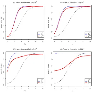
Let λ1= [ λ1 ]and λ2= [ λ2 λ3 ]0. Here, we set αν=0.05 forν=1,2,3 and consider all the cases whenθRT_≥θUT_{. In Figure 1, the power of the UT, RT and PTT are}

plotted againstλ1for selected values of[λ2,λ3].Asλ1grows large, power of all tests grow large too. Although the power of the UT and RT are increasing to 1 asλ1is increasing, the power of the PTT is increasing to a value that is less than 1. The analytical findings in the previous Section supports these graphical results.

Since the UT, RT and PTT are defined based on the knowledge ofβ₂= [ _{β2 β3} ]0_,

0 2 4 6 8 10

0.0

0.2

0.4

0.6

0.8

1.0

λ1

power of the test

(a) Power of the test for λ2=[0,0]T

ΠUT

ΠRT

ΠPTT

0 2 4 6 8 10

0.0

0.2

0.4

0.6

0.8

1.0

λ1

power of the test

(b) Power of the test for λ2=[1,1]T

ΠUT

ΠRT

ΠPTT

0 2 4 6 8 10

0.0

0.2

0.4

0.6

0.8

1.0

λ1

power of the test

(c) Power of the test for λ2=[2,2] T

ΠUT

ΠRT

ΠPTT

0 2 4 6 8 10

0.0

0.2

0.4

0.6

0.8

1.0

λ1

power of the test

(d) Power of the test for λ2=[4,4] T

ΠUT

ΠRT

ΠPTT

Figure 1: Graphs of power of the tests as a function ofλ1for selected values ofλ2and

α1=α2=α3=α=0.05.

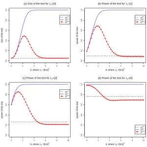
the size and power of each test are plotted againstbsuch thatλ2= [ b b ]0in Figure 2.

0 2 4 6 8 10

0.0

0.2

0.4

0.6

0.8

1.0

b, where λ2 =[b,b]T

size of the test

(a) Size of the test for λ1=[0]

ΠUT

ΠRT

ΠPTT

0 2 4 6 8 10

0.0

0.2

0.4

0.6

0.8

1.0

b, where λ2 =[b,b]T

power of the test

(b) Power of the test for λ1=[1]

ΠUT

ΠRT

ΠPTT

0 2 4 6 8 10

0.0

0.2

0.4

0.6

0.8

1.0

b, where λ2 =[b,b]T

power of the test

(c) Power of the test for λ1=[2]

ΠUT

ΠRT

ΠPTT

0 2 4 6 8 10

0.0

0.2

0.4

0.6

0.8

1.0

b, where λ2 =[b,b]T

power of the test

(d) Power of the test for λ1=[4]

ΠUT

ΠRT

ΠPTT

Figure 2: Graphs of power of the tests as a function ofλ2for selected values ofλ1and

α1=α2=α3=α=0.05.

b<qis more realistic. The properties of some of the proposed test statistics have already been studied and used to define preliminary test and shrinkage M-estimators by Ahmed et. al. (2006) [21].

7 Concluding Remarks

In this paper, the proposed M-tests do not depend on the assumptions on the distribution of the population. The asymptotic sampling distributions of the UT, RT and PT follow univari-ate noncentral chi-square distribution under the alternative hypothesis when the sample size

is large. However, the sampling distribution of the PTT is a bivariate noncentral chi-square distribution as there is a correlation between the UT and PT. Note that there is no such cor-relation between the RT and PT. The new R code defined in Yunus and Khan (2009b) [15] is used for the computation of the distribution function of the bivariate noncentral chi-square distribution to evaluate the power function of the PTT .

The RT has the largest power among the three tests, but it also has the largest size. On the other hand the UT has smallest size, but it has the smallest power as well except when

λ1=n

1

2β₁orλ₂=n12β₂is large. So, both UT and RT fail to achieve the highest power and

lowest size simultaneously. The PTT has smaller size than the RT. It also has higher power than the UT, except for very large values ofλ1 orλ2. Therefore if the prior information is not far away from the true value, that is,λ2is near 0 (small or moderate) the PTT has smaller size than the RT and higher power than the UT. Hence is it a better compromise between the two extremes. Since the prior information is coming from previous experience or expert knowledge, it is reasonable to expect λ2 should not be too far away from 0, although it may not be 0, and hence the PTT demonstrate a reasonable domination over the other two tests in more realistic situation.

Acknowledgements

The authors thankfully acknowledge valuable suggestions of Professor A K Md E Saleh, Carleton University, Canada that helped improve the content and quality of the results in the paper.

A Appendix A

The following asymptotic results of [9, p.221]), [12, 14] are used in deriving the distribution of the proposed tests. For simplicity, we assumeSis known or consider the nonstudentized M-estimator, so we omit condition M1 of [9, p.217] and letSn=Sin equation (5.5.29) of

[9, p.221]. Thus,

real numbers, asngrows large,

sup{n−12|M_n

1{(a,b) + (t1,t2)} −Mn1(a,b) +nγ(Q11t1+Q12t2)|: |t1| ≤n−

1

2_{K,|t2| ≤n}−12_K}→p _{0, (A.1)}

sup{n−12_|Mn

2{(a,b) + (t1,t2)} −Mn2(a,b) +nγ(Q21t1+Q22t2)|: |t1| ≤n−

1

2K,|t₂| ≤n−12K}→p 0. (A.2)

• Underβ₁=0,β₂=0, asngrows large,

n−12



 Mn1(0,0)

Mn2(0,0)

  d

→Np

    0 0  _,σ2

0 

 Q11 Q12

Q21 Q22  



_{, (A.3)}

whereNp(·,·)represents ap-variate normal distribution with appropriate parameters

andK∈ℜ.

Proof of part (i) of Theorem 1. By equations (A.1) and (A.2), we find

n−12_Mn

1(0,β˜2) = n−

1 2_Mn

1(0,β2)−n

1 2_γQ

12(β˜2−β2) +op(1)and (A.4)

n−12_Mn

2(0,β˜2) = n−

1 2_Mn

2(0,β2)−n

1 2_γQ

22(β˜2−β2) +op(1) (A.5)

underH?

0.Then, we obtain

n−12M_n

1(0,β˜2) =n−

1 2M_n

1(0,β2)−n−

1 2Q

12Q−221Mn2(0,β2) +op(1) (A.6)

by equations (2.5), (A.4) and (A.5) after some simple algebra. Further, the distribution of n−1_2M

n1(0,β˜2) under H0? is the same as the distribution of n−12M_n

1(0,0)−n− 1

2Q₁₂Q−1

22Mn2(0,0)underH0:β1=0,β2=0 using equation (A.6) and the fact that the distribution ofMn1(a,b)under θ=a,β=b is the same as that of

Mn1(θ−a,β−b)whenθ=0,β=0,and similarly forMn2(0,0)(c.f. [22, p.322]).

Therefore, utilizing equation (A.3), underH?

0:β1=0 asn→∞,the proof of part (i) of Theorem 1 is completed.

The proof for part (ii) of Theorem 1 is obtained in the same way as in part (i).

Proof of part (ii) of Theorem 2. UnderH0:β1=0,β2=0,with relation to (A.1) and (A.2), 

 n−

1 2M_n

1(0,0)

n−1 2M_n

2(β˜1,0)  ₋

  n−

1 2M_n

1(0,0)

n−1 2M_n

2(0,0)

 ₊



 0

n12γQ₂₁β˜

1  _→p

  0

0 

Note also that underH0,

n−12M_n

1(β˜1,0) =n−

1 2M_n

1(0,0)−n 1 2γQ₁₁β˜

1+op(1) (A.8)

and definition (2.6) reduce equation (A.8) to

n−12Q

21Q−111Mn1(0,0) =n 1 2γQ

21β˜1+op(1). (A.9)

Therefore, underH0, equation (A.7) becomes 

 n−

1 2M_n

1(0,0)

n−1_2M

n2(β˜1,0)

 ₋



 n−

1 2M_n

1(0,0)

n−1_2M

n2(0,0)−n 1

2Q₂₁Q−1

11Mn1(0,0)



 _(A.10)

=

  n−

1 2M_n

1(0,0)

n−12M_n 2(β˜1,0)

 ₋



 Ir 0

−Q₂₁Q−₁₁1 Is

    n−

1 2M_n

1(0,0)

n−12M_n 2(0,0)

 _→p

  0

0 

_{. (A.11)}

Now utilizing the contiguity of probability measures (see [23, Ch.7]) under{Kn}to those

underH0, the equation (A.11) implies that h

n−1_2M0

n1(0,0) n

−1_2M0

n2(β˜1,0)

i₀

under{Kn}is asymptotically equivalent to the random vector



 Ir 0

−Q₂₁Q−1 11 Is

    n−

1 2M_n

1(0,0)

n−1 2M_n

2(0,0)

 

underH0.But the asymptotic distribution of the above random vector under{Kn} is the

same as 

 Ir 0

−Q21Q−111 Is

    n−

1 2M_n

1(−n− 1

2λ₁,−n−12λ₂)

n−12M_n 2(−n−

1

2λ₁,−n−12λ₂)

 

underH0by the fact that the distribution ofMn1(a,b)underθ=a,β=bis the same as that

ofMn1(θ−a,β−b)underθ=0,β=0,and similarly forMn2(0,0)(c.f. [22, p.322]).

Note that underH0, with relation to (A.1) and (A.2), 

 n−

1 2M_n

1(n− 1

2λ₁,n−12λ₂)

n−12M_n 2(n−

1

2λ₁,n−12λ₂)

 ₌

  n−

1 2M_n

1(0,0)

n−12M_n 2(0,0)

 

+



 γ(Q11λ1+Q12λ2)

γ(Q₂₁λ1+Q22λ2)  ₊

  op

op

 _.

Hence, by equation (A.3), underH0, 

 n−

1 2M_n

1(n− 1

2λ₁,n−12λ₂)

n−12M_n 2(n−

1

2λ₁,n−12λ₂)

 _→Np

 



 γ(Q11λ1+Q12λ2)

γ(Q₂₁λ1+Q22λ2)  _,σ2

0 

 Q11 Q12

Q₂₁ Q₂₂

 

 _.

(A.13)

Thus, asn→∞,the distribution of h

n−1 2M0_n

1(0,0) n

−1 2M0_n

2(β˜1,0)

i₀

under{Kn}isp-variate normal with mean vector



 Ir 0

−Q21Q−111 Is  



 γ(Q11λ1+Q12λ2)

γ(Q21λ1+Q22λ2)  ₌



 γ(Q11λ1+Q12λ2)

γ(Q22−Q21Q−111Q12)λ2  

and covariance matrix 

 Ir 0

−Q21Q−111 Is  _σ2

0 

 Q11 Q12

Q21 Q22   

 Ir 0

−Q21Q−111 Is  

0

=σ2₀



 Q11 0 0 Q?₂

 _.

Since the two statisticsn−12M_n

1(0,0)andn− 1 2M_n

2(β˜1,0)are uncorrelated, asymptotically, they are independently distributed normal vectors.

Proof of part (i) of Theorem 2. UnderH0:β1=0,β2=0,with relation to (A.1) and (A.2), (2.5), (A.9),

  n−

1 2M0

n1(0,β˜2)

n−12M0

n2(β˜1,0)

 ₋



 Ir −Q12Q−221

−Q21Q−111 Is     n−

1 2M_n

1(0,0)

n−12M_n 2(0,0)

 _→p

  0

0  _.(A.14)

Now utilizing the contiguity of probability measures under{Kn} to those underH0, the

equation (A.14) implies that h

n−12M0

n1(0,β˜2) n

−12M0

n2(β˜1,0)

i₀

under{Kn}is asymptotically equivalent to the random vector



 Ir −Q12Q−221

−Q₂₁Q−1

11 Is

    n−

1 2M_n

1(0,0)

n−1 2M_n

2(0,0)

underH0.But the asymptotic distribution of the above random vector under{Kn} is the

same as _

 Ir −Q12Q−221

−Q₂₁Q−₁₁1 Is

    n−

1 2M_n

1(−n− 1

2λ₁,−n−12λ₂)

n−1 2M_n

2(−n− 1

2λ₁,−n−12λ₂)

 

underH0.Then, equation (4.2) follows from equation (A.13) after some algebra. Since

n−12M_n

1(0,β˜2)andn−

1 2M_n

2(β˜1,0)are uncorrelated, asymptotically, they are independently distributed normal vectors.

B Appendix B

Write the second term on the right hand side of the equation (5.4) as

Z _∞

χ2

r,α₁

Z _∞

χ2

s,α₃

φ?(w1,w2)dw1dw2= [1−Hr(χ2r,α1;θ

UT_)][1−H

s(χ2s,α3;θ

PT_{)], (B.1)}

whereHr(χ2r,α1;θ

UT_{) =∑}∞

j=0∑∞δ1=0

(1−ρ2₎r/2_Γ(r

2+j)ρ2j

Γ(r2)j! γ ?

µ

r

2+j+δ1, χ2

r,α1

2(1−ρ2₎

¶

e−θUT/2_(θUT_/2)δ1

δ1!

andHs(χ2s,α3;θ

PT_{) =∑}∞

k=0∑∞δ2=0

(1−ρ2₎s/2_Γ(s

2+k)ρ2k

Γ(s

2)k! γ ?

µ

s

2+k+δ2, χ2

s,α₃

2(1−ρ2₎

¶

e−θPT/2_(θPT_/2)δ₂

δ2! .

Note, Hr(χ2r,α1;θ

UT_)≥G

r(χ2r,α1;θ

UT_{) and H}

s(χ2s,α3;θ

PT_)≥G

s(χ2s,α3;θ

PT_{). Equality is}

achieved whenρ=0,or whenλ1=0 andλ2=0.

Consider all the cases whenθRT_≥θUT _{andρ6=0. So, using equation (B.1), we write}

equation (5.4) as

ΠPT T(λ1,λ2) ≤ ΠRT(λ1,λ2)[1−ΠPT(λ1,λ2)] +ΠUT(λ1,λ2)ΠPT(λ1,λ2). (B.2)

Equality in equation (B.2) is achieved when bothλ1andλ2are 0.Obvious,ΠPT T(λ1,λ2)<

ΠRT_(λ

1,λ2)−ΠPT(λ1,λ2)v2for 0≤v2<1,and it follows thatΠPT T(λ1,λ2)≤ΠRT(λ1,λ2) for anyλ1andλ2.Equality holds when bothλ1andλ2are 0.

Rewrite equation (5.5) as

Z_∞

χ2

r,α₁

Z_∞

χ2

s,α₃

φ?(w1,w2)dw1dw2

= 1−Hr(χ2r,α1;θ

UT_)−H

s(χ2s,α3;θ

PT_{) +}

Z _χ2

r,α₁

0

Z _χ2

s,α₃

0 φ

?_(w

1,w2)dw1dw2. (B.3)

Whenλ2is not large but not 0 andλ1is sufficiently large, the first term on the right hand side of the equation (5.4) becomes G(χ2

s,α3;θ

second and fourth terms on the right hand side of the equation (B.3) becomes 0 because

θUT _{is large. Also, note thatH}

s(χ2s,α3;θ

PT_)>G

s(χ2s,α3;θ

PT_{). So,Π}PT T _<ΠUT _{=1 for}

sufficiently largeλ1and not so largeλ2 (6=0).

Letα1=α2=α3=α. Whenλ2=0 andλ1is sufficiently large, the first term on the right hand side of the equation (5.4) becomes 1−αbecauseθRT_{is large. BothH}

r(χ2r,α;θUT) andRχ2r,α

0

Rχ2

s,α

0 φ?(w1,w2)dw1dw2 of the equation (B.3) become 0 whileHs(χ2r,α;θPT) be-comes 1−α. So,ΠPT T _=ΠUT _{=1 whenλ}

1is sufficiently large andλ2=0. In the same manner, we observe results given in (c)-(f) below

(a) Whenλ2(6=0) is not large andλ1is sufficiently large, then,ΠPT T<ΠUT =1.

(b) Whenλ2=0 andλ1is sufficiently large, then,ΠPT T =ΠUT =1.

(c) Whenλ1is not large butλ2is sufficiently large, then,ΠPT T <ΠUT =1.

(d) Whenλ1=0 andλ2is sufficiently large, then,ΠPT T =ΠUT =α.

(e) When bothλ2andλ1are sufficiently large, then,ΠPT T <ΠUT.

(f) When bothλ1andλ2are 0, thenΠPT T =ΠUT =α.

Also, we find from equations (5.4) and (B.1) thatΠPT T _>ΠUT_if ΠRT Hr(χ2r,α;θUT)>

Hs(χ2s,α;θPT)

(1−ΠPT₎ .

We observe, when bothλ1andλ2are 0, theΠUT =ΠRT =ΠPT T =α.Asλ1grows larger andλ2fixed at 0,ΠUT,ΠRT andΠPT T grow larger and approach 1 withΠUT ≤ΠPT T ≤

ΠRT_.

Whenλ1=0 andλ2is small (6=0), we findΠPT T(0,λ2)>ΠUT(0,λ2) =αif Π

RT

α >

Hs(χ2s,α;θPT)

(1−ΠPT₎ .Asλ1grows larger andλ2fixed at some small positive vector,ΠUT andΠRT grow large and approach 1, however,ΠPT T _{grows large and approaches a value less than}

1. Note,ΠUT_≤ΠPT T _≤ΠRT _{when 0<λ}

1≤q1, andΠPT T ≤ΠUT ≤ΠRTwhenλ1>q1, whereq₁is some positive vector.

REFERENCES

[2] Khan, S. and Saleh, A.K.Md.E. (2001). On the comparison of the pre-test and Stein-type estimators for the univariate normal mean,Statistical Papers,42, 451-473.

[3] Bechhofer, R.E. (1951). The effect of preliminary test of significance on the size and power of certain tests of univariate linear hypotheses. Ph.D. Thesis (unpublished), Columbia Univ.

[4] Bozivich, H., Bancroft, T.A. and Hartley, H. (1956). Power of analysis of variance test procedures for certain incompletely specified models,Ann. Math. Statist.,27, 1017 -1043.

[5] Tamura, R. (1965). Nonparametric inferences with a preliminary test, Bull. Math. Stat.,11, 38-61.

[6] Saleh, A.K.Md.E. and Sen, P.K. (1982). Non-parametric tests for location after a pre-liminary test on regression,Communications in Statistics: Theory and Methods,11, 639-651.

[7] Saleh, A.K.Md.E. and Sen, P.K. (1983). Nonparametric tests of location after a pre-liminary test on regression in the multivariate case, Communications in Statistics: Theory and Methods, 12, 1855-1872.

[8] Lambert, A., Saleh A.K.Md.E. and Sen P.K. (1985). Test of homogeneity of intercepts after a preliminary test on parallelism of several regression lines: from parametric to asymptotic,Comm. Statist.,14, 2243-2259.

[9] Jurecˇckov´a, J. and Sen, P.K. (1996).Robust Statistical Procedures Asymptotics and Interrelations.John Wiley & Sons, US.

[10] Huber, P.J. (1981).Robust Statistics.Wiley. New York.

[11] Arnold, S.F. (2005). Nonparametric statistics. Summer School in Statistics for As-tronomers and Physicists. Penn State University.

[12] Sen, P.K. (1982). On M-tests in linear models,Biometrika,69, 245-248.

[14] Jureˇckov´a, J. (1977). Asymptotic relations of M-estimates and R-estimates in linear regression model,Ann. Statist.,5, 464-72.

[15] Yunus, R. M. and Khan, S. (2009b). The bivariate noncentral chi-square distribution - a compound distribution approach, Working Paper Series, SC-MC-0902, Faculty of Sciences, University of Southern Queensland, Australia.

[16] Wilcox, R.R. (2005).Introduction to Robust Estimation and Hypothesis Testing. El-sevier Inc. US.

[17] Montgomery, D.C., Peck, E.A. and Vining G.G. (2001).Introduction to linear regres-sion analysis(3rd ED.). Wiley. New York.

[18] Muirhead, R.J. (1982),Aspects of multivariate statistical theory, US: John Wiley & Sons.

[19] Gunst, R.F. and Webster, J.T. (1973). Density functions of the bivariate chi-square distribution,Journal of Statistical Computation and Simulation A,2, 275–288.

[20] Wright, K. and Kennedy, W.J. (2002). Self-validated computations for the probabil-ities of the central bivariate chi-square distribution and a bivariateF distribution,J. Statist. Comput. Simul.,72, 63–75.

[21] Ahmed, S.E., Hussein, A.A. and Sen, P.K. (2006). Risk comparison of some shrinkage M-estimators in linear models.Nonparametric Statistics,18, 401-415.

[22] Saleh, A.K.Md.E. (2006).Theory of Preliminary test and Stein-type estimation with applications. John Wiley & Sons. New Jersey.

[23] H´ajek, J., ˇSid´ak, Z. and Sen, P.K. (1999).Theory of Rank Tests.Academia Press. New York.

not be copied or emailed to multiple sites or posted to a listserv without the copyright holder's express written