Other uses, including reproduction and distribution, or selling or
licensing copies, or posting to personal, institutional or third party
websites are prohibited.
In most cases authors are permitted to post their version of the
article (e.g. in Word or Tex form) to their personal website or
institutional repository. Authors requiring further information
regarding Elsevier’s archiving and manuscript policies are
encouraged to visit:
Estimating the diffuse attenuation coefficient from optically active constituents
in UK marine waters
M.J. Devlin
a,*, J. Barry
b, D.K. Mills
b, R.J. Gowen
c,1, J. Foden
b, D. Sivyer
b,
N. Greenwood
b, D. Pearce
b, P. Tett
daCatchment to Reef Research Group, ACTFR, James Cook University, Townsville, Queensland 4811, Australia bCentre for Environment, Fisheries and Aquaculture Science, Pakefield Rd, Lowestoft, NR33 0HT, England, UK
cAquatic Systems Group, AFESD, Department of Agriculture and Rural Development, Newforge Lane Belfast BT9 5PX, Northern Ireland, UK dSchool of Life and Health Sciences, University of Napier 10 Colinton Road Edinburgh EH10 5DT, Scotland, UK
a r t i c l e
i n f o
Article history: Received 16 June 2008 Accepted 15 December 2008 Available online 25 December 2008
Keywords: light attenuation
suspended particulate matter chlorophyll
CDOM
a b s t r a c t
We report a study of the attenuation of submarine Photosynthetically Active Radiation (PAR) in relation to the concentrations of Optically Active Constituents (OACs) in a range of water types around the United Kingdom. 408 locations were visited between August 2004 and December 2005. The diffuse attenuation coefficient (Kd) was estimated from profiles of downwelling PAR. Concentrations of Suspended
Partic-ulate Matter (SPM) were measured gravimetrically and concentrations of phytoplankton chlorophyll (chl) were measured by fluorometrically. Chromophoric Dissolved Organic Matter (CDOM) was measured either by fluorescence or as its proxy, salinity.
Several empirical models forKdas a function of SPM, chlorophyll and CDOM were fitted to the data set. It
was found that including all three explanatory variables (CDOM, chlorophyll and SPM) gave a slightly better fit for coastal and offshore waters, whereas a fit based only on SPM and chlorophyll worked well for transitional (estuarine) waters. The use of SPM as a single predictor ofKdin all water types resulted in
only 3% loss of accuracy.
The effect of seasonal variations in the light climate and the OACs was investigated with high frequency data from moorings in the Thames embayment and Liverpool Bay.Kdwas estimated from data recorded
from pairs of vertically separated PAR sensors. Using the empirical models to estimateKdfrom these
OACs showed that reliable estimates of attenuation could be made throughout the year, with some scatter of estimatedKdabout observedKdduring the growing season.
The reliability of these findings was validated by non-linearly fitting of a mechanistic model, based on semi-intrinsic optical parameters, to the spatial data set. Estimated values of absorption cross-section and scattering cross-section were in good agreement with the literature, and help to justify parameter values obtained from the empirical models.
Ó2009 Elsevier Ltd. All rights reserved.
1. Introduction
Effective strategies for managing nutrient enrichment in marine waters require an understanding of how different types of waters respond to nutrient inputs. Susceptibility to nutrient enrichment is controlled by a wide variety of processes (Painting et al., 2005). Recent reviews (Cloern, 1999, 2001) of the developing conceptual scientific model of marine eutrophication has shown a clear
progression from simple dose–response models, typically used in freshwater science, to a more realistic model that identifies direct and indirect responses that are governed by ‘filters’. The variables that form the filter are the underwater light climate, the degree of horizontal exchange, the tidal mixing regime, the extent of pelagic and benthic grazing, and biogeochemical processes such as deni-trification. Light limits growth of phytoplankton and is a first order determinant of the response of phytoplankton to nutrient input in the sea. The supply of photosynthetically active radiation (PAR) for phytoplankton growth in the sea is a product of the input of solar radiation at the surface and its reduction by optically active compounds (OACs) through absorption and scattering (Kirk, 1994), which itself is increased by higher phytoplankton concentrations.
*Corresponding author.
E-mail address:[email protected](M.J. Devlin).
1Present address: Fisheries and Aquatic Ecosystems Branch, AFESD, Agri-Food and Biosciences Institute, Newforge Lane Belfast BT9 5PX, Northern Ireland, UK.
Contents lists available atScienceDirect
Estuarine, Coastal and Shelf Science
j o u r n a l h o m e p a g e : w w w . e l s e v i e r . c o m / l o c a t e / e c s s
These internal feedbacks make the behaviour of light difficult to quantify. The rate at which light diminishes with depth is generally measured as the diffuse vertical attenuation coefficient for down-wards PAR,Kd.
The UK has a large coastal zone, and many of its transitional and coastal waters are turbid and optically complex. Most of the marine waters in the UK are thought to be light limited, influ-encing the maximum rate of primary production (Devlin et al., 2008). Knowledge of the underwater light climate can help to predict the specific susceptibility of different marine environ-ments to the adverse effects of nutrient enrichment, and thus focus costly measures for reducing nutrient load on those water bodies that are mostly likely to be improved in quality (Jago et al., 1993). However, it is not feasible to characterise all UK marine water bodies by direct measurement of Kdat different times of
year and under a range of tidal stirring or freshwater discharge conditions. Instead, we have sought a model that relates variation in diffuse attenuation to differences in the amounts of Optically Active Components (OACs).
This paper reports observations ofKdand OACs in a variety of
estuarine, coastal and offshore waters around the United Kingdom. The data have been used to estimate empirical attenuation cross-sections (thek*) in the equation:
Kd ¼ k*wþk*CDCDOMþKPH* chloroþk*SPSPM (1)
where the terms on the right hand side of the equation refer to the effects of water ðk*
wÞ, ‘yellow substance’ or coloured dissolved
organic matter(CDOM) measured as fluorescence, phytoplankton photosynthetic pigments measured as the concentration of chlo-rophyll (chloro), and suspended particulate matter (SPM). The Equation(1) is derived from the following mechanistic equation (Kirk, 1994) in terms of beam absorption coefficients, a, and
absorption cross-sections,a*:
Kd ¼
m
1d a ¼
m
1d
awþa*CD½CDOM þa*PH½chloro þa*SPM½SPM
(2)
on the assumption that the mean cosine for downwards PAR photons,
m
d, can be treated as a constant over the variety of watertypes, solar angles and cloud covers encountered during the study. An alternative to this assumption (from Kirk, 1994 and Bowers et al., 2000) is to make the cosine depend onbeam scatteringby SPM:
m
1 d ¼ffiffiffiffiffiffiffiffiffiffiffiffiffiffiffiffiffiffiffiffiffiffiffiffiffiffiffiffiffiffiffiffiffiffiffiffiffiffiffiffiffiffiffiffiffiffiffiffiffi
1þkm
b*
SP½SPM
=a
r
(3)
whereb*
SPis ascattering cross-sectionandkmis a parameter to be
discussed further in ‘Methods’. These equations are termed ‘mechanistic’ because they synthesise the ‘apparent optical prop-erty’, diffuse attenuation, from more fundamental ‘inherent optical properties’ than can be measured in the laboratory. In fact, the beam absorbance sections and the beam scattering cross-section used here are not truly inherent, because they depend on the spectrum of submarine illumination, which is likely to vary amongst the water types studied.
The aim of the paper is to report observations of attenuation and OACs in UK salt waters, and derive a practically useful, theo-retically informed, model for predictingKd. The analysis presented
here extends the results and interpretation reported by Devlin et al. (2008)which aimed chiefly to estimate typical attenuations in each of the UK water types that have been identified for the Water Framework Directive (Vincent et al., 2002; Rogers et al., 2003).
2. Methods
2.1. Sampling strategy
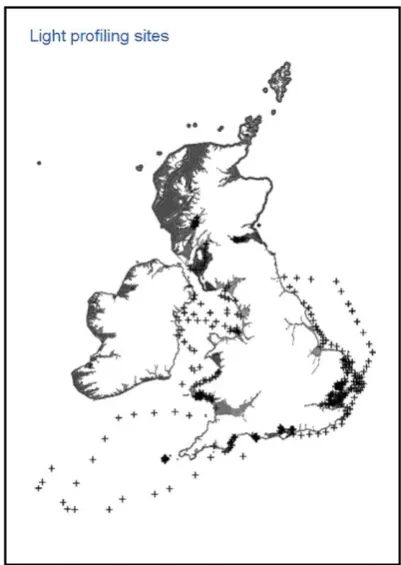
Surveys carried out between August 2004 and December 2005 aimed at spatial extensiveness and visited a total of 408 locations (Fig. 1). Sampling took place from a variety of observational plat-forms, providing data at a range of spatial and temporal resolutions. Platforms used included: small vessels (inflatables and EA survey vessels) for spatial sampling in inshore areas; larger research vessels (ABFI R.V. Corystes and CEFAS Endeavour) for spatial sampling in deeper offshore regions; and bridges for some estua-rine sites. In July 2005, sampling was undertaken in the Clyde sea area and Irish Sea (including Irish coastal waters of the western Irish Sea) during a Department of Agriculture and Rural Develop-ment (DARD) RV Corystes cruise. Sampling sites were identified as eithertransitionalorcoastalwater types as designated by the Water Framework Directive (CEC, 2000), or offshore waters. Transitional waters are estuaries, characterised by salinities less than 30. Coastal waters are defined as those waters within 1 nm of the coast (3 nm from an extended coastal baseline in Scotland). All sites sampled seaward of the WFD defined coastal waters and were grouped as offshore waters.
[image:3.595.326.527.433.716.2]Temporal variation of light measurements were accounted for by using daily averages of nearly-continuous observations by instrumented buoys (www.cefas.co.uk/monitoring) at 2 sites in shallow (<20 m) coastal locations (Fig. 1). Each buoy houses a suite of autonomous instruments measuring a range of variables at high frequency (daily to hourly) at fixed-point locations (http://map. cefasdirect.co.uk/smartbuoyweb/StaticMapPage.asp). Both sites (Liverpool Bay and the Warp Anchorage in the Thames estuary)
were in regions of freshwater influence close to major riverine nutrient sources and were generally well mixed with regard to density. However, intermittent periods of stratification, mainly due to salinity, have been observed in Liverpool Bay where SmartBuoy observations were carried out as part of the Proudman Oceano-graphic Laboratory (POL) Liverpool Bay Coastal Observatory pro-gramme (www.cefas.co.uk). Data from the Thames buoy covered the period from December 2000 until December 2005; that from Liverpool Bay started in November 2002 and ended in November 2005.
2.2. Sampling methods
At each survey site profiles were obtained using a stainless steel protective frame containing a solid state logger (Cefas ESM2) sampling at 2 Hz interfaced to a range of sensors that was lowered by hand or using a hydrographic winch. Sensors used included a Falmouth Scientific Instruments (Falmouth, USA) CT sensor, a Druk (Origin) pressure sensor, a Seapoint (Origin) chlorophyll fluorometer and optical backscatter sensor and a LI-COR (LI-192) Underwater Quantum Sensor measuring downwelling PAR irradi-ance. Care was taken to minimise the influence of shading on measurements made by the irradiance sensors by profiling through a constant light field; i.e. a profile could be carried out either on the illuminated or the shaded side of the platform, provided conditions were consistent and the instruments did not go into and out of shadow. Surface and near bottom water samples, were collected using Niskin type water bottles for the estimation of SPM, chloro-phyll, CDOM and salinity. Offshore water samples were collected in 5-l water bottles mounted on a rosette sampler from the near surface (2 m) and near bottom (2–3 m above the seabed). At deep sites a water sample was collected from 25 m, which corresponded, to the lower limit of the irradiance profile.
The SmartBuoy instruments were in general similar to those described above. The main differences were as follows. Sensors interfaced to the logger are sampled at 1 Hz for two 10-min bursts each hour. Data for these 10-min bursts are averaged and are referred to as ‘burst means’. 2–3 water samples of 150 ml each, for subsequent gravimetric analysis of SPM, were collected each week of deployment using an automated water sampler (AquaMonitor, Envirotech, Virginia, USA). Sensors and samplers were positioned at fixed depths between 1 and 2 m. Two upwards pointing LI-COR quantum irradiance sensors are used to measure downwelling PAR irradiance at 1 and 2 m depths.
2.3. Laboratory analyses
Salinity, chlorophyll, SPM and CDOM analyses were carried out on samples collected from spatial surveys using Niskin bottles and on water samples collected on the SmartBuoy. For salinity, samples were collected in 200 ml medical bottles and stored prior to anal-ysis at Cefas. Salinity was measured using a Guildline Autosal 8400b laboratory salinometer.
Chlorophyll was measured by passing up to 250 cm3of seawater through Whatman GF/F glass fibre filters. These filters were extracted overnight in 90% acetone neutralised with NaHCO3 in
darkness in a refrigerator as described byTett (1987). After centri-fugation, extract fluorescence was measured using a Tuner Designs Model 10 – AU – 005 CE fluorometer before and after acidification with 8% HCl. This was used to calculate concentrations of ‘chloro-phyll a’. The fluorometer had been calibrated using pure solutions of chlorophyll a (Sigma Chemical Co, ORIGIN) with concentration determined spectrophotometrically. Replicate measurements of chlorophyll had typical standard errors of around 10%.
Samples for SPM were preserved with mercuric chloride and returned to the laboratory for filtration. The concentration of SPM was measured by gravimetric analysis using the method of Strick-land and Parsons (1972). Known volumes of water were filtered through pre-weighed Whatman GF/C glass fibre filters in the laboratory. The filters were then dried and re-weighed to calculate the total suspended sediment collected on the glass fibre filters. Suspended load concentration was calculated from differences in the weight (Strickland and Parsons, 1972).
Samples for CDOM were collected from Niskins in high-density 1l polyethylene (HDPE) bottles, filtered through a 47-mm 0.2-
m
m membrane and the resulting filtrate kept in amber bottles and refrigerated prior to analysis. Samples were allowed to reach room temperature. CDOM fluorescence was measured at room temper-ature using a Turner Fluorometer Model 10 Series fitted with a 310–390 nm excitation filter and 410–600 nm emission filter, with 10-327R attenuator plate. The method is described in detail inFoden et al. (2008). CDOM units have been revised from N.Fl.U. to be quoted as S.Fl.U. – standardised fluorescence units, as differentiated from normalised fluorescence units, byFerrari and Dowell (1998).In the absence of CDOM data on the SmartBuoy measurements, salinity was used as a proxy for CDOM. A strong, negative corre-lation coefficient of CDOM to salinity (r2¼0.81) is reported in Foden et al. (2008). The linear relationship described in this paper (y¼ 0.174xþ6.288) was used to calculate CDOM from the high frequency salinity data collected with the SmartBuoy observations.
2.4. Calibration of sensors
The fluorometers used in this study, for profiling and moored observations, are designed to provide a linear response between chlorophyll concentration and fluorometer voltage. Although cali-brated by the manufacturer, in practice a calibration based upon field data is required (Mills and Tett, 1990).
The equation
X ¼ ðFfo=EÞ (4)
was used to predict chlorophyll concentration X mg m3where
E¼compound fluorescence emission coefficient m3
(mg pigment)1(V or arbitrary units);
F¼fluorometer output in volts or arbitrary units in the case of the Seapoint fluorometer;
fo¼fluorometer output in the absence of extractable pigment.
The primary aim in calibrating the fluorometer was the esti-mation of the compound fluorescence coefficient, E. Linear regression of fluorometer voltage on observed pigment concen-tration gives slopeEand an intercept defined by the manufacturer. Pigment data for the calibration regressions were obtained by collecting water samples immediately after each profile or from samples collected alongside the SmartBuoy fluorometers at the beginning and end of deployments.
Concentrations of SPM were regressed (least squares linear regression) against corresponding values of optical backscatter (OBS) recorded as manufacturer calibrated FTU. Values of SPM concentration were estimated from the equation:
SPM ¼ ðFTUþintercept=slopeÞ (5)
2.5. Calculation ofKd(PAR)
The attenuation coefficient, Kd (m1) of photosynthetically
available radiation (PAR), was calculated using the Lambert–Beer equation (Dennison et al., 1993) from vertical profiles of downw-elling irradiance (Equation(6)). The light attenuation coefficient relates to light penetration depth and the quantity of suspended and dissolved substances.
Kd ¼ dðlnðEzÞÞ=dz; approximated as :
D
ðlnðEzÞÞ=D
z (6)where Kdrepresents the attenuation coefficient for downwards
PAR, and ln (Ez) is the natural logarithm of PAR at depth z (z increasing downwards).
Surface light attenuation was not measured through the profiling. Profiles which showed evidence of contamination by cloud cover or inconsistent match ups between the top down and bottom up profiles were discarded.
To be consistent with the method of calculating mean concen-trations of SPM,Kdwas derived from the whole light profile and
surface mixed layer profile in vertically mixed and stratified waters respectively.Kdwas calculated from the slope of irradiance and
depth. Typically, the relationship between logarithmic PAR and depth was linear. Areas of scatter were excluded from the vertical profile. These were most commonly seen at the region of hyper-exponential decay near the surface as some wavelengths of light are more quickly absorbed and the photon distribution is forced near the surface. Linear fitting of the irradiance values was taken to the depth at which light fell to the instrument’s minimum level of detection.
In the case of Smartbuoy observations,Kdwas taken from the
natural logarithm of the ratio of irradiances at 1 m and 2 m depth. From the measurements of irradianceEd(z) at two depths theKd
was calculated as follows:
Kdm1¼ lnEdð1Þ
Edð2Þ
=zð2Þ zð1Þ (7)
2.6. Empirical models
The empirical models developed below were chosen so that they provided good empirical explanations of variation inKd. As
such, the model parameters did not have any particular physical meaning.
There were three explanatory variables for diffuse attenuation, the concentrations of the OACs coloured dissolved organic matter (CDOM), phytoplankton pigments, and suspended particulate matter (SPM). Pigments were measured as chlorophyll (chloro), and CDOM was measured as fluorescence.
Three types of model were tested. These were the Log-Normal Model, the Linear Model and the Gamma Generalised Linear Model (seeDobson, 2002). The three types of models were fitted using all possible subsets of the explanatory variables. However, they are illustrated with the full set of explanatory variables.
1. Log-Normal. For this model, it is assumed that Kdhas a
log-normal distribution and is predicted by:
lnðKdÞ ¼
b
0þb
CDlnðCDOMÞ þb
PHlnðchloroÞ þb
SPlnðSPMÞþerror
(8)
where the error is normally distributed with mean zero and variance
y
2 and the parameters,b
0;
b
CD;b
CHandb
SP; areesti-mated by their respective maximum likelihood estimates
b
b
0;bb
CD;bb
CHandbb
SP. In order to obtain predictions ofKdon theuntransformed scale, the standard back-transformation was used
~
Kd ¼ exp
ln
~
Kdþb
y
2=2
(9)
where lnðKbd ¼ b
b
0þbb
CDlnðCDOMÞ þbb
PHlnðchloroÞ þbb
SPlnðSPMÞÞand b
y
2is the estimate of the residual variance on the log scale.2. Linear. This is the model of Equation (1), involving the assumption that the effect of each OAC on attenuation is line-arly additive:
lnðKdÞ ¼
b
0þb
CDCDOMþb
CHchloroþb
SPSPMþerror (10)where the error is normally distributed with mean zero and variance
s
2. Note that theb
parameters here are equivalent tothe empirical attenuation cross-sections (thek*) defined in(1). The predicted value is then,
b
Kd ¼ b
b
0þbb
CDCDOMþbb
PHchloroþbb
SPSPM (11)3. Gamma GLM. In this case it was assumed thatKdhas a
log-normal distribution; its mean was modelled using a General-ised Linear Model with errors that have a Gamma distribution and a log-link between the explanatory variable Kdand the
linear predictor. The predicted values ofKdfrom this model
were simply the exponential of the estimated values from the linear predictor:
b
Kd ¼ expb
b
0þbb
CDCDOMþbb
PHchloroþbb
SPSPM(12)
A succession of models using each of these three approaches was calculated to investigate how the different combinations of the variables performed in the prediction ofKd. Fitting was carried out
using the R statistical package (R Development Core Team, 2006). To test the accuracy of the models, a cross validation measure (referred to here as D), was used. It calculates the percentage difference between predicted and observed values ofKdwith lower
values indicating greater accuracy.Dis defined as:
D ¼ 100X
n
j¼1 KbdjK
j d bKdj
(13)
whereKbdjis the value predicted for observationjusing all of the data except thejth observation,Kdjis thejth observation ofKdandn
is the number of cases in the prediction data set.
2.7. Theoretical model
The theoretical model introduced in Equations (2) and (3)is built from the (semi)-inherent optical properties of absorption and scattering. It can be restated as follows:
Kd ¼
m
1o
ffiffiffiffiffiffiffiffiffiffiffiffiffiffiffiffiffiffiffiffiffiffiffiffiffi
a2þk
mab q
(14)
a ¼ awþa*CDCDOMþa*PHchloroþa*SPSPM (15)
b ¼ b*
SPSPM (16)
Three parameters were known a priori. The first of these,
m
ois themean cosine of downwelling light in the absence of scattering. It was given the value of 0.85, suitable for southern UK waters in the middle part of the day in summer. The coefficient calledkmwas expanded byBowers et al. (2000)as 0.425
m
o0.19, resulting ina value 0.171. The value of seawater absorption for PAR was taken as
aw ¼0:02 m1. The remaining four parameters (the a* and b* values) were estimated by non-linear fit of the Equation set(14)– (16)to the whole-survey data set. The fit was done in the statistical package R (R Development Core Team, 2006) using a simple least squares error criterion and a Nelder-Mead optimisation criterion in the functionoptim. Ninety-five percent confidence intervals for the model parameters were calculated using bootstrapping with 1000 re-samples (Manly, 1998).
3. Results
The survey data set used for development of the empirical models contained 382 full rows, each row contained Kd, SPM,
CDOM and chlorophyll observations. The fitting of the full theo-retical model was pruned of any row with missing observations. Four cases were removed as their SPM values were large outliers, not corresponding with water type, which we assume could have
been caused by measurement error. This left 273 complete rows, from the original 382. However, parameter estimates for models, were derived using all data rows that were complete for these models, which provided more data for the simplified models than for the complete models. Data rows were further characterised by water type: transitional waters (62 complete rows), coastal waters (185 complete rows), and offshore waters (26 complete rows).
High frequency data from the SmartBuoys was extracted from January 2001 to 2005 for Thames embayment and from January 2003 to 2005 for Liverpool Bay. Measurements of chlorophyll, SPM and salinity were taken for the optically important components of
Kd. Data rows with missing observations were deleted, leaving 1091
rows for the Thames and 843 rows for Liverpool Bay.
3.1. Empirical modelling using survey data
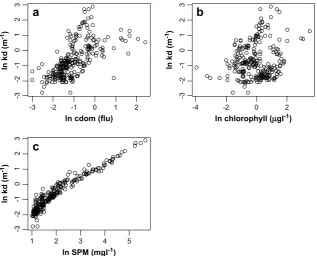
The logarithmic relationships (over the whole data set) between
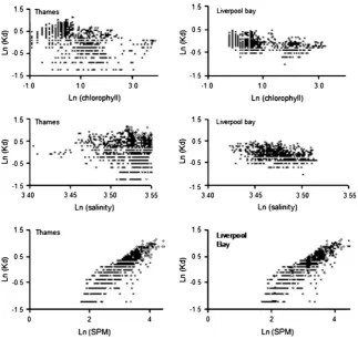
Kdand CDOM, chlorophyll and SPM are illustrated inFig. 2. By far
the strongest and clearest relationship was betweenKdand SPM,
with transformed SPM explaining 91% of the variance in log-transformedKd. The patterns were less clear for chlorophyll and
CDOM. Nevertheless, both chlorophyll and CDOM had some explanatory power, and although the weakest relationship, between ln (chlorophyll) and ln (Kd) explained only 3% of the
variance in the latter, the correlation was statistically significant (p¼0.006).
Results from fitting the empirical models are given inTables 1 and 2. In addition to fitting to the full data set, the models were also fitted separately to each of the three sets of category-specific data. Comparison of the models using the full data set identified the single variable SPM, as being the most important variable for estimatingKd. Comparing the model scenarios, using a combination
of OACs demonstrated that the models incorporating CDOM and SPM, and the model with all three variables (CDOM, SPM and chlorophyll), performed the best. There was little to choose between the Generalised Linear and the Log-Normal models. The
-3 -2 -1 0 1 2
-3
-2
-1
0
1
2
3
ln cdom (flu)
ln kd (m
-1)
-4 -2 0 2
-3
-2
-1
0
1
2
3
ln chlorophyll (µgl-1)
ln kd (m
-1)
1 2 3 4 5
-3
-2
-1
0
1
2
3
ln SPM (mgl-1)
ln kd (m
-1)
a
b
[image:6.595.146.464.486.742.2]c
lowest value ofD¼22.6 for the log-normal model using the full data set of CDOM and SPM values can be interpreted as saying that
Kdvalues were predicted with approximately 23% relative accuracy.
In terms of future prediction, the Linear, Log-Normal and Gener-alised Linear Model performed equally well.
In general, the models fit better in the transitional and offshore waters than in the coastal waters.As expected, models for separate water types generally perform better than a single model fitted to the whole data set. Percentage improvements of about 6% for the transitional and offshore waters would seem to justify fitting different models to these areas.
[image:7.595.32.284.134.384.2]For both coastal waters and offshore waters, the full model fitted slightly better than the reduced models. In transitional waters, the reduced model of chlorophyll and SPM performed very similarly to the full model. There was little difference between the perfor-mances of the three model types.
Table 2includes the parameter estimates for three of the best combinations of explanatory variables for the linear model. For offshore and coastal there is little difference between the perfor-mance of the models with SPM and CDOM and with SPM and chlorophyll (though the former models are about 1% better). For transitional waters, there is a 3.4% improvement in relative prediction for the model with SPM and chlorophyll. We suggest the models below as the good predictive models for each category:
Offshore : Kbd ¼ 0:145þ0:156CDOMþ0:083SPM (17)
Coastal : Kbd ¼ 0:1155þ0:5639CDOMþ0:0654SPM (18)
b
Kd ¼ 0:2290þ0:0456chloroþ0:0652SPM (19)
Note units of measurement for CDOM, SPM and chlorophyll are S.FL.U, mg L1, and
m
g L1respectively.From the 95% confidence intervals inTable 2, we can see that CDOM and SPM coefficients for the offshore and coastal categories are statistically different. The intercept terms for all three models are statistically significantly different from zero.
3.2. Testing of empirical models against high frequency data
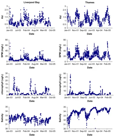
Time-series plots ofKd, salinity, chlorophyll and SPM are shown
inFig. 3. In general, attenuation was greater during winter, when there was high suspended particulate matter, most likely due to the higher rainfall and runoff. Spring and summer blooms of chloro-phyll and fluctuations in salinity, had apparently little effect on the attenuation signal. These patterns are clarified in the scatter plots of ln (Kd) against the OACs inFig. 4. Ln(SPM) explained 99% of the
variation inKd.
Calculation ofD(Table 3) using high frequency data, demon-strated that SPM remained the best single predictor ofKd. For the
Thames embayment, the best model was the linear model with chlorophyll and SPM as explanatory variables. For Liverpool Bay the models with salinity (as a proxy for CDOM), SPM and chlorophyll fitted slightly better than the CDOM and SPM model.
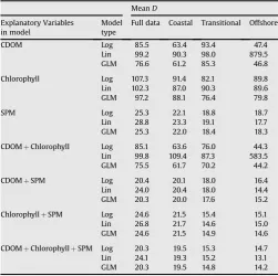
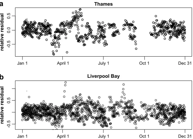
As an illustration, relative residuals were calculated from the log-normal model with SPM as the explanatory variable for both Liverpool Bay and Thames moorings (Fig. 5). The relative residuals (i.e. the components ofD) were plotted against day of year. They show that the model fits reasonably well throughout most of the year, with higher deviation during the phytoplankton bloom season (March–May). This would suggest that even though SPM is the best Table 1
Values of the fit statisticDfor the survey data. Within each part of the table, the three rows give results for the model categories: Log¼log-normal, Lin¼linear; GLM¼gamma Generalised Linear Model.Dis the mean of the absolute relative deviations, expressed as a percentage.
MeanD Explanatory Variables
in model
Model type
Full data Coastal Transitional Offshore
CDOM Log 85.5 63.4 93.4 47.4
Lin 99.2 90.3 98.0 879.5 GLM 76.6 61.2 85.3 46.8
Chlorophyll Log 107.3 91.4 82.1 89.8
Lin 102.3 87.0 90.3 89.6 GLM 97.2 88.1 76.4 79.8
SPM Log 25.3 22.1 18.8 18.7
Lin 28.8 23.3 19.1 17.7 GLM 25.3 22.0 18.4 18.3
CDOMþChlorophyll Log 85.1 63.6 76.0 44.3 Lin 99.8 109.4 87.3 583.5 GLM 75.5 61.7 70.2 44.2
CDOMþSPM Log 20.4 20.1 18.0 16.4
Lin 24.0 20.4 18.0 14.4 GLM 20.3 20.0 17.6 15.2
ChlorophyllþSPM Log 24.6 21.5 15.4 15.1 Lin 26.8 21.7 14.6 15.0 GLM 24.6 21.5 14.9 14.6
[image:7.595.30.556.605.768.2]CDOMþChlorophyllþSPM Log 20.3 19.5 15.3 14.7 Lin 24.1 19.3 15.2 13.1 GLM 20.3 19.5 14.8 14.2
Table 2
Estimated linear model coefficients for the three models, 95% confidence intervals(in brackets) and residual degrees of freedom for the survey data set.
df b0 bsp
SPM (m2g1) Transitional 77 0.338 (0.205,0.472) 0.065 (0.063,0.067) Coastal 249 0.188 (0.013,0.051) 0.064 (0.068,0.071) Offshore 46 0.001 (0.081,0.083) 0.066 (0.058,0.074)
b0 bCD bsp
CDOM (S.Fl.U)þSPM (m2g1) Transitional 60
0.129 (0.179,0.079) 0.58 (0.415,0.746) 0.064 (0.062,0.066) Coastal 189 0.116 (0.17,0.061) 0.564 (0.383,0.745) 0.065 (0.064,0.067) Offshore 26 0.145 (0.169,0.121) 0.156 (0.038,0.273) 0.083 (0.076,0.089)
b0 bPH bsp
Chloro (m2mg1)
þSPM (m2g1) Transitional 76 0.229 (0.098,0.360) 0.046 (0.024,0.067) 0.065 (0.063,0.067) Coastal 246 0.004 (0.048,0.040) 0.016 (0.006,0.038) 0.070 (0.068,0.071) Offshore 43 0.036 (0.095,0.167) 0.028 (0.109,0.054) 0.064 (0.056,0.073)
b0 bCD bPH bsp
CDOM (S.Fl.U)þchloro (m2mg1)
þSPM (m2g1) Transitional 59 0.222 (0.064,0.379) 0.003 (
single predictor over time forKd, there are periods during the year
when the simple linear relationship breaks down and that the high concentrations of chlorophyll present in the spring and summer blooms do influence the prediction ofKd. It is still suitable to use
SPM as a single predictor for the majority of the year without a significant loss of accuracy, however, during spring and summer blooms, it would be more appropriate to use the mixed model of chlorophyll and SPM in the Thames and the full model (CDOM, SPM and chlorophyll) for Liverpool Bay.
3.3. Theoretical model
Parameter estimates and bootstrapped 95% confidence intervals from the non-linear fit of the theoretical model are given inTable 4. We also calculated the value of theD-statistic for the non-linear model. This came to 27.5. If we compare this with the values in the last row ofTable 1for the empirical models, we can see that these empirical models perform between 3 and 7% better than the theoretical model.
4. Discussion
The most striking and useful outcome from the empirical analysis is that SPM concentration is the most important predictor of diffuse attenuation. A linear regression using only SPM estimated
Kdhas a mean error of 30% over the whole data set, falling to 18% in
the case of the offshore data set. Using logarithmic regression or a GLM reduced the error for the whole data set slightly, to 27–28%. Adding in the effects of chlorophyll and CDOM reduced the linear model error only to 26% for the whole data set and 13% for the offshore data set (23% and 14–15% for the other models). This supports work byCloern, 1987, May et al., 2003, Painting et al., 2005, Weeks et al., 1993, Lund-Hansen, 2004, Xu et al., 2005, Devlin et al., 2008that strong correlations betweenKdand SPM imply that
light attenuation, particularly in UK estuaries, is primarily a func-tion of suspended sediment concentrafunc-tions.
There are three reasons for this dominance. Firstly, SPM influ-ences the optical signal by way of scattering as well as absorption of light. Secondly, the data set included a very wide range of SPM
0 0.5 1 1.5 2 2.5 3
Jan-03 Jul-03 Feb-04 Aug-04 Mar-05 Oct-05
Date
Kd
0 0.5 1 1.5 2 2.5 3
Jan-01 Nov-01 Sep-02 Jun-03 Apr-04 Feb-05
Date
Kd
0 20 40 60 80
Jan-03 Jul-03 Feb-04 Aug-04 Mar-05 Oct-05
Date
SPM (mg/L)
0 20 40 60 80
Jan-01 Nov-01 Sep-02 Jun-03 Apr-04 Feb-05
Date
SPM (mg/L)
0 5 10 15 20 25 30
Jan-03 Jul-03 Feb-04 Aug-04 Mar-05 Oct-05
Date
chlorophyll (ug/L) 0
10 20 30 40 50
Jan-01 Nov-01 Sep-02 Jun-03 Apr-04 Feb-05
Date
Chlorophyll (ug/L)
30 31 32 33 34 35
Jan-03 Jul-03 Feb-04 Aug-04 Mar-05 Oct-05
Date
Salinity
30 31 32 33 34 35
Jan-01 Nov-01 Sep-02 Jun-03 Apr-04 Feb-05
Salinity
Date
[image:8.595.113.491.87.537.2]Liverpool Bay Thames
concentrations, from 3.7 to 110 mg/L. Thirdly, many UK waters are turbid, with a high load of suspended particles. In this they may be contrasted with other waters. The Baltic Sea, for example, has an optical signal dominated by CDOM because of the large freshwater content, whereas under non-tidal and fjordic conditions, the SPM load is comparatively small (Kratzer et al., 2003; Kratzer and Tett, in press).
There is little to choose in prediction performance between any of these models. The fact that the gamma GLM model performs similarly to the log-normal model suggests that the log-normal model is a good model forKdas the log-normal model is one of the
family of gamma GLM models. However in terms of simplicity, we recommend the use of the linear models as they are relatively easy to populate with no need to calculate error. There is little or no loss of accuracy in choosing the linear model for all water types.
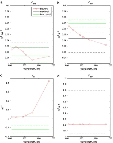
Fig. 6compares: the parameter values estimated by fitting the mechanistic model to the whole data set; those estimated by the empirical multiple linear regression of coastal water attenuation on the three OACs; and values taken fromBowers et al. (2000), which were based on relevant literature and studies in the Irish Sea and the Clyde Sea. The Bowers et al values for SPM refer to mineral suspended particulate matter, whereas the values from the present work refer to total SPM (i.e. including some organic component).
‘Mech-all’ inFig. 6refers to parameters of the mechanistic, or theoretical, model fitted to the entire data set, which gave esti-mates ofa*PHand a*SP (Table 4). ‘Lin-coastal’ inFig. 6 refers to
parameters from a linear fit of the coastal waters data set forKdto
[image:9.595.131.455.88.394.2] [image:9.595.32.284.529.767.2]CDOM, chlorophyll and SPM; the result of this fit was a set of attenuation cross-sections (Table 2, final rows), which have been converted to absorption cross-sections in Fig. 6(a) and (b) by multiplying by
m
¼0.8, a value of the mean cosine estimated from Fig. 4.High frequency data from the Smartbuoy observations described in scatter plots of log-transformedKdon log-transformed optically active components.Table 3
Values of the fit statisticDfor the high frequency data. Within each part of the table, the three rows give results for the model categories: Log¼log-normal, Lin¼linear; GLM¼gamma Generalised Linear Model.Dis the mean of the absolute relative deviations, expressed as a percentage. Thames is Thames embayment and Liv. Bay denotes Liverpool Bay marine area.
Explanatory variables in model Model type
Thames full data
Liv Bay full data
CDOM [sal] Log 36.2 38.2
Lin 36.7 38.1
GLM 36.7 38.3
Chlorophyll (m2mg1) Log 34.1 37.9
Lin 36.4 43.9
GLM 34.5 38.0
SPM (m2g1) Log 18.1 22.4
Lin 18.4 23.0
GLM 18.2 22.4
CDOM[sal]þChlorophyll (m2mg1) Log 34.2 34.7
Lin 36.5 53.5
GLM 34.6 34.8
CDOM [sal]þSPM (m2g1) Log 18.0 21.7
Lin 18.3 21.9
GLM 18.0 21.6
Chlorophyll (m2mg1)þSPM (m2g1) Log 17.9 22.3
Lin 17.8 23.2
GLM 17.9 22.2
CDOM [sal]þChlorophyll (m2mg1) þSPM (m2g1)
Log 17.7 21.4
Lin 17.7 21.3
Equation(3)and mean values of the optically active components. This was also done to get the water absorption (aw) inFig. 6(c) from the multiple regression intercept in Table 2. The value for water absorption in the mechanistic model was that assigned before fitting. The scattering cross-section (b*SP) inFig. 6(d) could not be
estimated for the ‘lin-coastal’ data set.
Taking account of the confidence limits, both estimates ofa*PHin
Fig. 6(a) agree well with the values from Bowers et al. The offshore waters value inTable 2is also in good agreement. The transitional waters value seems high; although the confidence limits overlap the Bowers et al. values for short wavelengths, it is more likely that it is the longer wavelength values that are typical of these waters. The mechanistic model value ofa*SP. is in good agreement with
the values from Bowers et al.; the linear model’s value for coastal water is significantly higher, and this is also the case for the values for transitional and offshore waters inTable 2. In the case of the coastal and offshore waters data sets, a possible explanation relates to the linear model’s estimate of the absorption,aw, of pure water. As shown in Fig. 6(c) for coastal waters, this was 0.15 m1 compared with 0.02 m1in the mechanistic model and the data set of Bowers et al. The negative intercept of the (multiple) linear regression has to be compensated by a higher value in the coeffi-cient for the main optically active component, which is SPM. This explanation does not work for transitional water, for whichawwas estimated asþ0.18.
Finally, the estimate of scattering cross-section from the mechanistic model agrees well with the value from Bowers et al., although within wide confidence limits.
The generally agreement between values estimated with the mechanistic model and those in Bowers et al. (2000) gives us confidence in the observations and the methods used to analyse the data resulting from them. The differences between the mechanistic model values and those obtained by multiple linear regression can be explained by the fitting of a linear model to graphs that may have some curvilinear or bimodel aspects, as can be seen inFig. 2. Nevertheless, we can have confidence in the results from the empirical model because of these comparisons as well as from the results inTable 2showing that the linear multiple regressions ofKd
on CDOM, chlorophyll and SPM show a relative percentage prediction error of less than 25% for the full data set, and less than 20% when the data set is divided between water types. Finally we can conclude from Table 2 that a simple linear model relating attenuation only to SPM will often be adequate for the estimation of
Kdin UK coastal waters, with less than 30% prediction error in the
case of the full data set and less than 20% for the individual type data sets.
The outcomes of the models demonstrate that single sets of model parameters can be used effectively across a wide range of water types and times of year. The remaining error in the model fits, and the resulting uncertainty in parameter values, is likely from two main groups of causes. The first is the result of variability in the submarine light field that is not taken into account in any of the models. Such variability derives from: (1) seasonal and diel changes in the angle of incidence of solar radiation on the sea surface, which introduce variation into the parameter
m
0that we have treated asfixed; and (2) variations in the spectral distribution of submarine light, which depend on the optical type of water. The latter contribute to uncertainty in the model parameters, because the truly intrinsic parameters are functions of wavelength whereas we have treated them as constant for PAR.
The second group of causes relates to the inherent properties of the OACs themselves. Scattering per unit mass of particulate matter depends on particle size, so we might expect regional variability in
a*SPandb*SP. Despite this variability we found a clear, all-regions,
relationship betweenKdand [SPM]. Another source of variation
may have arisen from regional or seasonal differences in the type of
relative residual
Thames
-0.5
0.0
0.5
Jan 1 April 1 July 1 Oct 1
relative residual
-0.5
0.5
Jan 1 April 1 July 1 Oct 1
Dec 31
Dec 31
Liverpool Bay
.
.
a
[image:10.595.147.461.91.317.2]b
[image:10.595.41.293.716.767.2]Fig. 5. High frequency data from Smartbuoy instruments: Time-series of residuals for the log-normal model with SPM as the explanatory variable for both Thames (a) and Liverpool Bay (b).
Table 4
Parameter estimates and 95% bootstrapped confidence intervals for the theoretical non-linear model in Equations(14)–(16).
Parameters (units) Estimate and 95% confidence interval
a*
CD 0.054 (0.028, 0.121)
a*
PHm2mg1 0.028 (0.008, 0.036) a*
SP(m2g1) 0.043 (0.019, 0.054) b*
planktonic micro-alga and hence in the wavelength-dependent values ofa*PH.
Testing of the empirical (linear, multiple regression) model over time using a high frequency data set has shown that the model works well over the whole year, with a small loss of accuracy in the summer months as shown in the residual plots in Fig. 5. The additional scatter during these months may be the result of an increased contribution of phytoplankton chlorophyll to the OACs, and should be investigated further using the data available from moorings.
The variation in residual values between Thames and Liverpool Bay are different, with the Thames experiencing higher residual
values in May and June, indicating a later spring bloom with more persistent summer blooms (Fig. 5). Liverpool Bay has high residual values for only a short period of time, typically in April, indicating that chlorophyll influences the predictive model only during very short spring bloom peaks.
Devlin et al. (2008)investigate a large data set of SPM values from different water types to calculate the adequacy of the predictive models over different water types. This work illustrated the strong relationship between SPM andKdin UK waters. This optical
[image:11.595.107.481.87.558.2]temporal variation of SPM and Kdas shown by the variation in
residual concentrations during the spring and summer bloom. However, the very high accuracy attributed to the SPM model would warrant that the predictive models could be used with a high degree of confidence over the majority of the year and possibly to hindcast light from historical SPM levels in UK marine waters.
In conclusion, this study provides important new data on OACs, and their effects onKd, in UK estuaries and coastal waters that not
only inform of factors controlling the underwater light field but are also relevant to interpreting remotely-sensed emergent light (Sathyendranath and Platt, 1997;Bowers and Binding, 2006). From the analysis of spatial and temporal light data from UK marine waters, it is clear that SPM concentration is the most important predictor of diffuse attenuation. Simple linear regressions using SPM only estimatedKdwith a mean error of 30% for the whole data
set, falling to 18% in the case of the offshore data set. Using loga-rithmic regression or a GLM reduced the error for the whole data set slightly, to 27–28%. The slight decrease in error using a combi-nation of the other OAC’s is significant, however the strong and persistent correlations between Kd and SPM supports current
thought that light attenuation, particularly in UK estuaries, is primarily a function of suspended sediment concentrations.
Finally it is worth noting that these optically active compounds can also provide important diagnostic indicators of a wide variety of natural and anthropogenic stressors that impinge on estuaries and coastal waters (Gallegos, 2001; Gallegos and Jordan, 2002; Kratzer and Tett, in press).
Acknowledgements
This work was funded by the Defra contract (E2202) Eutro-phication Thematic Programme and by DARD. The authors would like to thank Environment Agency staff who assisted in field work, the Captain, Officers and Crew of the RV Corystes for their assis-tance during the Clyde Sea and Irish Sea survey in July 2005. The assistance of Mr B. Stewart (DARD) Dr. K. Kennington and Miss A Harrison (University of Liverpool) during the RV Corystes cruise is gratefully acknowledged. The views expressed in this paper are those of the authors and do not necessarily reflect those of DEFRA, DARD and the EA.
References
Bowers, D.G., Harker, G.E.L., Smith, P.S.D., Tett, P., 2000. Optical properties of a region of freshwater influence (the Clyde Sea). Estuarine, Coastal and Shelf Science 50, 717–726.
Bowers, D.G., Binding, K.E., 2006. The optical properties of mineral suspended particles: a review and synthesis. Estuarine and Coastal and Shelf Science 67, 219–230. Cloern, J.E., 1987. Turbidity as a control on phytoplankton biomass and productivity
in estuaries. Continental Shelf Research 7 (11/12), 1367–1381.
Cloern, J.E., 1999. The relative importance of light and nutrient limitation of phytoplankton growth: a simple index of coastal ecosystem sensitivity to nutrient enrichment. Aquatic Ecology 33, 3–16.
Cloern, J.E., 2001. Our evolving conceptual model of the coastal eutrophication problem. Marine Ecology Progress Series 210, 223–253.
Dennison, W.C., Orth, R.J., Moore, K.A., Stevenson, J.C., Carter, V., Kollar, S., Bergstorm, P.W., Batiuk, R.A., 1993. Assessing water quality with submerged aquatic vegetation: habitat requirements as barometers of Chesapeake Bay health. Bioscience 43, 86–94.
Devlin, M., Mills, D.K., Gowen, R., Foden, J., Sivyer, D., Tett, P., 2008. Relationships between suspended particulate material, light attenuation and Secchi depth in UK marine waters. Estuarine Coastal and Shelf Science 79, 429–439. Dobson, A., 2002. An Introduction to Generalized Linear Models, second ed. CRC
Press, 245 pp.
Foden, J., Sivyer, D.B., Mills, D.K., Devlin, M.J., 2008. Spatial and temporal distribu-tion of chromophoric dissolved organic matter (CDOM) fluorescence and its contribution to light attenuation in UK waterbodies. Estuarine, Coastal and Shelf Science 79 (4), 707–717.
Ferrari, G.M., Dowell, M.D., 1998. CDOM absorption characteristics with relation to fluorescence and salinity in coastal areas of the southern Baltic Sea. Estuarine, Coastal and Shelf Science 47 (1), 91–105.
Gallegos, C., 2001. Calculating optical water quality targets to restore and protect submersed aquatic vegetation: overcoming problems in portioning the diffuse attenuation co-efficient for photosynthetically active radiation. Estuaries 24 (3), 381–397.
Gallegos, C.L., Jordan, T.E., 2002. Impact of the Spring 2000 phytoplankton bloom in Chesapeake Bay on optical properties and light penetration in the Rhode River, Maryland. Estuaries 25, 508–518.
Jago, C.F., Bale, A.J., Green, M.O., Howarth, M.J., Jones, S.E., McCave, I.N., Millward, G.E., Morris, A.W., Rowden, A.A., Williams, J.J., 1993. Resuspension processes and seston dynamics, southern North Sea. Philosophical Transactions of the Royal Society of London, Series A 343, 475–491.
Kirk, J.T.O., 1994. Light and Photosynthesis in Aquatic Ecosystems, seond ed. Cambridge University Press, UK.
Kratzer, S., Buchan, S., Bowers, D.G., 2003. Testing long-term trends in turbidity in the Menai Strait, North Wales. Estuarine Coastal and Shelf Science 56, 221–226.
Kratzer, S., Tett, P. Using bio-optics to investigate the extent of coastal waters – a Swedish case study. Hydrobiologia, in press.
Lund-Hansen, L.C., 2004. Diffuse attenuation coefficientsKd(PAR) at the estuarine
North Sea–Baltic Sea transition: time-series, partitioning, absorption, and scattering. Estuarine Coastal and Shelf Science 61, 251–259.
Manly, F.J., 1998. Randomization, Bootstrap and Monte Carlo Methods in Biology, second ed. Chapman and Hall, London, 399 pp.
May, C., Koseff, J., Lucas, L., Cloern, J., Schoellhamer, D., 2003. Effects of spatial and temporal variability of turbidity on phytoplankton blooms. Marine Ecology Progress Series 254, 111–128. .S.
Mills, D.K., Tett, P.B., 1990. Use of a recording fluorometer for continuous measurement of phytoplankton concentration. SPIE Proceedings 1269, 106–115.
Mills, D.K., Rutgers van der Loerf, M., Laane, R.W.P.M., Rees, J.M., 2002. Continuous measurement of suspended matter. Sea Technology 43 (10), 5 pp.
Painting, S., Devlin, M.J., Rogers, S., Mills, D.K., Parker, E.R., Rees, H.L., 2005. Assessing the suitability of OSPAR EcoQOs for eutrophication vs ICES criteria for England and Wales. Marine Pollution Bulletin 50, 1569–1584.
R Development Core Team, 2006. R: a Language and Environment for Statistical Computing. R Foundation for Statistical Computing, Vienna, Austria, ISBN 3-900051-07-0. Available from:http://www.R-project.org.
Rogers, S., Allen, J., Balson, P., Boyle, R., Burden, D., Connor, D., Elliott, M., Webster, M., Reker, J., Mills, C., O’Connor, B., Pearson, S., 2003. Typology for the Transitional and Coastal Waters for UK and Ireland. (Contractors: Aqua-fact International Services Ltd, BGS, CEFAS, IECS, JNCC). Funded by Scotland and Northern Ireland Forum for Environmental Research, Edinburgh and Environ-ment Agency of England and Wales, SNIFFER Contract ref: WFD07 (230/8030). 94 pp.
Sathyendranath, S., Platt, T., 1997. ‘‘Analytic model of ocean color’’. Applied. Optics 36, 2620–2629.
Strickland, J.D.H., Parsons, T.R., 1972. A Practical Handbook of Seawater Analysis, second ed. Bull. Fish. Res. Bd. Can.
Tett, P., 1987. The ecophysiology of exceptional blooms. Rapport et Proces-verbaux des Reunions. Conseil international pour l’Exploration de la Mer 187, 47–60. Vincent, C., Heinrich, H., Edwards, A., Nygaard, K., Haythornthwaite, K., 2002.
Guidance on Typology, Reference Conditions and Classification Systems for Transitional and Coastal Waters. CIS Working Group 2.4 (COAST), Common Implementation Strategy of the Water Framework Directive, European Commission, 119 pp.
Weeks, A.R., Simpson, J.H., Bowers, D., 1993. The relationship between concentra-tions of suspended particulate material and tidal processes in the Irish Sea. Continental Shelf Research 13, 1325–1334.