The facts about carbon and climate: a presentation of data for the reader's evaluation

The facts about carbon and climate

A presentation of data for the reader‟s evaluation

John Billingsley

Professor of Mechatronic Engineering University of Southern Queensland

QLD 4350, Australia [email protected]

Abstract— There is abundant factual data at repositories such as the U.S. Department of Energy Carbon Dioxide Information Analysis Center, which includes raw atmospheric measurement data from sites at numerous latitudes. Other reliable sites contain estimates of global industrial emissions and seasonal energy consumption. Further spectral data is available of the energy radiated into space. To perform a comparison of such disparate data, non-controversial conversions must be performed such as division by the area of the Earth.

The thrust of the paper is from the point of view of data analysis, correlation and statistical variation. No expertise in climatology or atmospheric physics is presumed beyond an assumption of the 'lapse rate', the rate at which convection maintains a decreasing temperature with increasing altitude.

The paper poses questions and avoids the contentious issues of interpreting the data or predicting futures. Any deductions or personal opinions are clearly declared and the conclusions are left to the reader.

Keywords-component; Greenhouse effect; climate change; observations; analysis; state space

I. THE OVERALL ISSUE

In the mind of the public, the issues of climate change and the reduction of carbon emissions have become inseparable. Logical considerations are clouded by political rhetoric, on the one hand by strident accusations of conspiracies and „swindles‟ by those wishing to make a political mark [1], on the other hand by acolytes trained in the camp of a would-be US president [2]. To suggest that the issue can be questioned in any way brings the risk of an accusation of being a „climate skeptic‟. Yet when the proposed remedy is so drastic, it is important to seek evidence not only that the malady exists, but that the regimen will actually have a beneficial effect on it.

Politicians of all persuasions have lent their agreement to many schemes, from emissions trading and geo-sequestration to wind farms. An international panel has pronounced that “we think we caused it” but the central question seems to have been overlooked:

“What is the degree of certainty that the measures proposed will have a beneficial effect on the future climate?”

This can be broken down into a chain of propositions for separate consideration:

1. Will the measures proposed have a significant effect on carbon emissions?

2. Will reducing carbon emissions have a measurable effect on the future atmospheric concentration of carbon dioxide?

3. How much influence does carbon dioxide have on the global temperature?

4. Would a temperature rise be detrimental or beneficial to the majority?

It is perhaps asking too much for an „answer‟ to these questions, but data can be drawn together from which some analysis can be made.

II. EMISSIONS REDUCTION

Although this falls outside the main scope of the paper, some thought can be given to the effectiveness of the measures proposed.

Substantial sums are being spent on „alternative energy‟. It must be questioned whether these power sources are truly alternative, or whether they are „additional‟. Their effect on emissions reduction can only result from a consequential reduction in the use of fossil fuel.

Will emissions trading actually reduce the use of fossil fuels, or merely change the location at which their carbon is released?

Perhaps direct regulation of the amount of coal that can be mined would have a more direct influence than either of these.

Sequestration into forest growth would appear to address the task, but once grown the timber must be protected forever from fire, having absorbed its total ration of carbon.

III. MANMADE EMISSIONS AND ATMOSPHERIC CARBON To make any sort of assessment of the effect of the first on the second, we have to reduce the data to a common denominator. Emissions are published as thousands of millions of tons per year, whereas atmospheric carbon is quoted in terms of „parts per million‟. Some calculations are necessary in order to compare them.

There is widespread ignorance on the question of “How much carbon is up there?” Yet the data is readily available. The atmospheric concentration of carbon dioxide has been monitored over many years. Although the data measured at Mauna Loa is the most often quoted, there are sites along a chain from Alaska to the South Pole.

For sites included in the Scripps database [4] the mean concentration for 2008 was 385 parts per million by volume. We must convert this to concentration by mass. The molecular weight of carbon dioxide is 12 + 2*16 = 44, compared with 2*16 = 32 for oxygen and 2*14 = 28 for nitrogen. The molecular weight for air falls between these at 29. To obtain figures for 'parts per million by weight' of the carbon within the carbon dioxide, the value of 385 is multiplied by 12/29 to give 160 parts per million.

At sea level, atmospheric pressure amounts to about 100 kilopascals, that is ten tonnes per square metre. The atmosphere is equivalent to this mass standing on each square metre of the Earth‟s surface. The mass of atmospheric carbon per square metre is thus 160 parts per million of ten tonnes, or 1.6 kilograms.

But what is really of interest is its rate of change. The carbon budget can be analysed by the technique of state-space system theory. A differential equation for atmospheric carbon a will express its rate of change in terms of any other „state variables‟ that can be identified. These will include global temperature T and the concentration a itself. Also involved will be inputs such as manmade emissions m and random effects r such as volcanic out-gassing. Effects such as biological uptake in the sea and on land will be included in the first function of temperature and concentration, though the parameters may be changed by land clearing.

r

m

T

a

f

dt

da







(

,

)

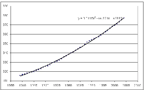
The annual Mauna Loa data on the Scripps site can be imported into an Excel table. A quadratic curve can then be fitted to the data, as shown in fig. 1, giving a method of estimating a smoothed gradient at any point.

The slope is thus .023*X - 44.321, where X is the year. For 2006 this is 1.817 ppm per year by volume. For 1970 it is 0.989 ppm per year.

For 2006, this translates into 1.817*10*12/29 = 7.5 grams per square metre per year.

For 1970 we see 0.989*10*12/29 = 4.1 gsm per year.

Figure 1. Mauna Loa data, parts per million by volume.

If we approximate the function by

qT

pa

T

a

f

(

,

)





then we can seek values of the coefficients by inspecting the gradient of a in differing years. But first we need to know the value of manmade emissions in terms of kilograms of carbon per year per square metre of the earth‟s surface.

Again we put trust in the data published by CDIAC [5]. An Excel plot of the more recent part is shown in fig. 2.

Figure 2. Carbon emissions from 1955. million tonnes.

The radius of the Earth is 6,378 kilometres, or 6.4 x 106 metres, so the area is 4 π r2 = 5.1 x 1014 square metres.

For carbon released in 2006, we take 8230 million tonnes being 8.2 x 1012 kg. We divide this by the area of the earth to get 16 x 10-3 kg = 16 grams per square metre.

For carbon released in 1970, we take 4076 million tonnes being 4.074 x 1012 kg. Divide this by the area of the earth to get 8 x 10-3 kg = 8 grams per square metre.

Finally the global temperature might come into play. Once more we take data from CDIAC [6] to plot in fig. 3 the global temperatures since 1955.

response to the state variables, it cannot be summed up as a simple proportion of the input.

Figure 3. Temperature anomaly, Celsius

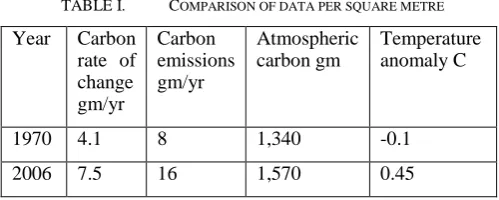
TABLE I. COMPARISON OF DATA PER SQUARE METRE

Year Carbon rate of change gm/yr

Carbon emissions gm/yr

Atmospheric carbon gm

Temperature anomaly C

1970 4.1 8 1,340 -0.1

2006 7.5 16 1,570 0.45

We must therefore explain a doubling of the „shortage‟ in terms of the increase in atmospheric carbon or the change in global temperature. If we discount the latter, we might expect that to halt the increase and hold values at their present level will require a halving of emissions.

However we can go further and question the potential „target‟ concentration if emissions remained the same. We have just two points to work from. With 325 ppm by volume in 1970 we had a rate of absorption of 4.1gm/sqm/yr. With 380 ppm by volume in 2006 we have a rate of absorption of 7.5 gm/sqm/yr. If we make the risky assumption that absorption rises linearly with concentration, from a false origin that would be 259 ppm, we would see a target of 518 ppm.

IV. HOW DOES CO2 AFFECT GLOBAL TEMPERATURE?

It can safely be asserted that the balance being sought is between radiant energy arriving from the sun and energy that is being radiated back into space from the Earth.

The term „Greenhouse Effect‟ has been used to explain the difference between the mean temperature of the surface of the Earth and the calculated equilibrium temperature of a „naked‟ object at this distance from the sun.

“Greenhouse” is a terrible misnomer. In the minds of a great number of the public, and I suspect of many politicians too, is the concept of a „layer of carbon dioxide‟ allowing radiation to pass inwards, but „trapping‟ heat by „reflecting‟ longer wavelengths back to the surface.

There is no layer of any „greenhouse gas‟ with the possible exception of the ozone formed high in the atmosphere. Instead the gases are uniformly diffused. Carbon dioxide can reflect

nothing. It certainly absorbs radiation at wavelengths in two significant bands, but must give up that heat to the ambient air before reradiating at an intensity corresponding to the ambient temperature.

The anomaly can be explained in terms of a „thermal horizon‟.

In a mist, there is a distance at which visibility falls to zero. Similarly, in a gas that is not completely transparent there is a distance at which radiation is reduced by a factor of e. This defines the absorption coefficient. Radiation intensity r can be expressed by the differential equation

kr

dx

dr

_

_

where the absorption coefficient is k. Now atmospheric density, and hence the absorption coefficient, falls off with height in an exponential manner, reducing by a factor of e each ten kilometres. So if we look at inward radiation where intensity increases with height, we will see that

r

ke

dh

dr



where H is 10 kilometres.

This has a solution that is an exponential of an exponential. The radiation is cut off quite sharply at a certain altitude. In the same way, when we look at the mirror of this equation for outgoing radiation, there will appear to be a distinct altitude from which radiation of any given wavelength can escape.

Now it is well known that the atmosphere gets cooler with altitude. This is termed the „lapse rate‟ and has a value of 6.5 centigrade degrees per thousand metres [7]. The effect is a thermodynamic one, of adiabatic cooling as air rises and expands.

The black body temperature of the Earth has been calculated as -18C, as opposed to a mean surface temperature of 14.5C. But at an altitude of 5,000 metres the atmosphere is 32.5 degrees cooler than at the surface. With this altitude as an effective „thermal horizon‟ there would be the necessary thermal balance.

The question then becomes, “What effect does an increase in carbon dioxide have on the altitude of the effective thermal horizon?”

It is a matter of concern that the IPCC reports [8] seem to be devoid of an analysis of the role played by the absorption coefficient in explaining the physics of the effects they have been assigned to analyse.

A more direct insight into the effect of „greenhouse gases‟ on radiation can be gained by looking at the spectrum of the emissions from Earth from space [9][10][11].

Figure 4. Copied with permission from Hearty[11]

Their agenda had nothing to do with the climate change controversy. Instead they were interested in the spectral signatures of planets that could support life.

It is clear that water vapour has the most significant effect, even on a clear day.

The carbon dioxide absorption band between 3 and 4 microns has little power associated with it. It is the 15 micron band that is significant. Here it appears that its effective emission temperature is around -55C, the temperature at the tropopause above which atmospheric temperature rises again. Indeed there is a „spike‟ at 15 microns, suggesting that the mid-band thermal horizon is well above the tropopause.

Total radiated energy is the area under this curve. To what extent would an increase in atmospheric carbon dioxide affect it?

V. WILL A GLOBAL TEMPERATURE RISE REALLY BE

CATASTROPHIC?

There are television advertisements predicting the extinction of the Great Barrier Reef and of catastrophic sea-level rises. Are they justified?

My opinion is that a temperature increase would see the gradual migration of species away from the tropics, or an

adaptation to the new conditions. Perhaps the Great Barrier Reef could then extend as far south as Brisbane.

Having spent my youth in Europe, I suspect that many would welcome some measure of warming.

But the evidence for such a temperature rise, or more particularly whether it could be influenced by carbon use policies, is something that must be debated on the available data.

VI. DEDUCTION AND SPECULATION

Rhetoric is rife on both sides of the argument. The Australian government has proposed a „Carbon pollution reduction scheme‟. Can carbon dioxide really be termed a pollutant, when it is so essential to all vegetation?

Whereas the measurement data quoted here appears to be objective and untarnished, estimates of global temperature are dependent on the method of their calculation.

five or ten years to minimize that variability, we find that global warming is continuing unabated."

To my eye, the Hansen data would appear to represent a plateau, or even a tendency to fall [13].

Indulge in some idle speculation. Fig. 4 emphasises the importance of ozone as a greenhouse gas. It is seen that the „shoulder‟ of the carbon dioxide band falls under its influence, while the central ozone trough makes an even greater contribution.

Is it possible that some of the temperature changes over the last twenty years can result from the phasing out the use of chlorofluorocarbons (CFCs) and the consequent strengthening of the high-level ozone layer?

Those wishing to see a reduction in global temperatures might seek the reinstatement of CFCs as propellants in aerosol cans.

VII. CONCLUSIONS.

There is an abundance of data, interpreted in a multitude of different ways. Analysis could be made of the deep annual cyclic variation in the far northern Point Barrow contribution to the Scripps data [4]. The variation each half year amounts to some 20 parts per million, five percent of the atmospheric total. Is it caused by leaf fall of the deciduous forests or by cyclic fossil fuel demands? There is no such variation at the latitude of New Zealand.

Much finer time-series analysis can be performed to correlate atmospheric concentration against events such as volcanic eruptions or the Indonesian peat-dome fires.

Already there is considerable research on the rate of biological uptake and the sensitivity coefficients of terms in the function that we have considered [14].

To see atmospheric carbon in proportion, note that carbon amounts to some 1.6 kilograms per square metre or 16 tons per hectare. A single wheat crop in one season can yield five tons per hectare, so time-constants are likely to be measured in years rather than centuries.

If this paper has come to any conclusion that might be regarded as contentious, it is that the matter is far from cut-and-dried. The „consensus‟ argument that „we can shout loudest so you have no right to question us‟ has many shameful historical examples. The paper puts forward no answer except an assertion that questions still remain.

REFERENCES

[1] Citizens Electoral Council, http://cecaust.com.au/ , viewed July 12, 2010

[2] The Climate Project, http://www.theclimateproject.org/ viewed July 12,

2010.

[3] NewGenCoal, http://www.newgencoal.com.au/ viewed July 12, 2010.

[4] Scripps Institution of Oceanography Monitoring Sites

http://cdiac.ornl.gov/trends/co2/sio-keel.html viewed July 13, 2010.

[5] Global Fossil-Fuel CO2 Emissions

http://cdiac.ornl.gov/trends/emis/tre_glob.html viewed July 13, 2010.

[6] Global and Hemispheric Temperature Anomalies - Land and Marine

Instrumental Records

http://cdiac.ornl.gov/trends/temp/jonescru/jones.html, viewed July 13, 2010.

[7] Mark Zachary Jacobson, Fundamentals of Atmospheric Modeling (2nd

ed.). Cambridge University Press, 2005. ISBN 0-521-83970-X

[8] IPCC home page http://www.ipcc.ch/ viewed July 13.

[9] JPL Atmospheric Infrared Sounder, http://airs.jpl.nasa.gov/ viewed July 14, 2010

[10] Mars Global Surveyor Thermal Emission Spectromether

http://tes.asu.edu/ viewed July 14, 2010

[11] Christensen, P.R., and J.C. Pearl, Thermal emission spectrometer

observations of Earth and Mars, J. Geophys. Res., 102, 10,875-10,880,

1997, figure at http://tes.asu.edu/TESCruise/marscruise.html viewed

July 14, 2010.

[12] Thomas Hearty, Inseok Song, Sam Kim and Giovanna Tinetti,

Mid-infrared properties of disk averaged observations of Earth with AIRS, The Astrophysical Journal 693 (2009) 1763

doi:10.1088/0004-637X/693/2/1763 image viewed at

http://iopscience.iop.org/0004-637X/693/2/1763/apj293285f4.html July 14, 2010.

[13] Annual Temperature Anomalies for Three Latitude Bands, 1900-2009

http://cdiac.ornl.gov/trends/temp/hansen/graphics/norlowsou.gif viewed July 15, 2010.

[14] The Aspen FACE experiment,