C
2011. The American Astronomical Society. All rights reserved. Printed in the U.S.A.
CHARACTERIZING THE VARIABILITY OF STARS WITH EARLY-RELEASE
KEPLER
DATA
David R. Ciardi1, Kaspar von Braun1, Geoff Bryden2, Julian van Eyken1, Steve B. Howell3, Stephen R. Kane1, Peter Plavchan1, Solange V. Ram´ırez1, and John R. Stauffer4
1NASA Exoplanet Science Institute/Caltech, Pasadena, CA 91125, USA 2Jet Propulsion Lab/Caltech, Pasadena, CA 91109, USA 3NOAO, 950 North Cherry Avenue, Tucson, AZ 85719, USA 4Spitzer Science Center/Caltech, Pasadena, CA 91125, USA
Received 2010 September 9; accepted 2011 January 17; published 2011 February 14
ABSTRACT
We present a variability analysis of the early-release first quarter of data publicly released by theKeplerproject. Using the stellar parameters from theKeplerInput Catalog, we have separated the sample into 129,000 dwarfs and 17,000 giants and further sub-divided the luminosity classes into temperature bins corresponding approximately to the spectral classes A, F, G, K, and M. Utilizing the inherent sampling and time baseline of the public data set (30 minute sampling and 33.5 day baseline), we have explored the variability of the stellar sample. The overall variability rate of the dwarfs is 25% for the entire sample, but can reach 100% for the brightest groups of stars in the sample. G dwarfs are found to be the most stable with a dispersion floor ofσ ∼0.04 mmag. At the precision ofKepler,>95% of the giant stars are variable with a noise floor of∼0.1 mmag, 0.3 mmag, and 10 mmag for the G giants, K giants, and M giants, respectively. The photometric dispersion of the giants is consistent with acoustic variations of the photosphere; the photometrically derived predicted radial velocity distribution for the K giants is in agreement with the measured radial velocity distribution. We have also briefly explored the variability fraction as a function of data set baseline (1–33 days), at the native 30 minute sampling of the public Keplerdata. To within the limitations of the data, we find that the overall variability fractions increase as the data set baseline is increased from 1 day to 33 days, in particular for the most variable stars. The lower mass M dwarf, K dwarf, and G dwarf stars increase their variability more significantly than the higher mass F dwarf and A dwarf stars as the time baseline is increased, indicating that the variability of the lower mass stars is mostly characterized by timescales of weeks while the variability of the higher mass stars is mostly characterized by timescales of days. A study of the distribution of the variability as a function of galactic latitude suggests that sources closer to the galactic plane are more variable. This may be the result of sampling differing populations (i.e., ages) as a function of latitude or may be the result of higher background contamination that is inflating the variability fractions at lower latitudes. A comparison of the M dwarf statistics to the variability of 29 known bright M dwarfs indicates that the M dwarfs are primarily variable on timescales of weeks or longer presumably dominated by spots and binarity. On shorter timescales of hours, which are relevant for planetary transit detection, the stars are significantly less variable, with ∼80% having 12 hr dispersions of 0.5 mmag or less.
Key words: stars: statistics – stars: variables: general
1. INTRODUCTION
Stars have long been known to vary in brightness, and photometric studies over the past centuries have revealed many classes of stars exhibiting a variety of variability (Pickering 1881). With interest in stellar variability growing tremendously in the last decade as ground-based and space-based surveys for exoplanets have gained momentum, under-standing the stellar photometric variability is even more crucial. Sources of stellar variability include pulsations, binarity, rotation, and activity (e.g., Eyer & Mowlavi 2008). Having a large sample of uniformly observed stars is vital in the categorization and characterization of the variability which can inform us about the stars themselves, their companions and companion rates, and their evolution. The fractions of stars that are found to be variable are dependent upon the sample of stars studied, the precision of the survey, the range of magnitudes over which the precision is matched, and the time duration of the survey (e.g., Eyer & Mowlavi2008; Howell2008). For example,
Hipparcos(with mmag precision and a completeness limit near
V=8 mag) found 10% of the stars in the sample to be variable (Eyer & Grenon1997; Eyer & Mowlavi2008), but the variability fraction depended upon both the stellar brightness and the stellar
type. Similar population and precision-dependent results have been found by survey programs intended for other purposes such as microlensing studies and transit surveys (e.g., OGLE: Wozniak & Szymanski 1998; HATNet: Hartman et al. 2004; WASP0: Kane et al.2005) as well as from general variability programs (e.g., BSVS: Everett et al.2002; FSVS: Huber et al.
2006; ASAS: Pojmanski2002).
As the surveys have become more sensitive, the fraction of stars observed to vary has been found to increase in a form which can be described by a power-law distribution directly proportional to the quality of the photometric precision (Howell 2008). This is a result of the current “best” survey precisions, time samplings, and survey durations probing ever deeper into the variability of stars but generally not reaching the astrophysical variability floor.
Spaced-based missions such asMOST(Matthews et al.1999),
CoRoT (Auvergne et al. 2009), and Kepler (Borucki et al.
The Astronomical Journal, 141:108 (21pp), 2011 April Ciardi et al.
micro-magnitude precision (6 hr timescale) for thousands of stars and has the potential to expand our knowledge of the lim-its of stellar variability.
Kepler was launched in 2009 March and began science operations in 2009 May. LikeCoRoT,Kepler does not study all stars within its field of view, but ratherKeplermonitors a specific set of∼150,000 target stars (Batalha et al.2010). Early work on the variability of stars in theKeplerdata set has been performed; these works have concentrated on the dwarf stars, periodicity, and flares (Basri et al.2010,2011; Walkowicz et al.
2011).
In 2010 June, theKeplerproject released to the public the first major time-series data product for the majority of the targets. We present a discussion of the data set (Section 2.1) and how it is divided into spectral and luminosity classes (Section 2.2). We primarily discuss the stellar variability of the sample on the timescale of the data set (33 days) and at the sampling rate of the data (30 minutes); we do explore briefly the variability as a function of the time baseline from 1 to 33 days. Discussions of the stellar photometric dispersions (Section3.1) and the variability fractions (Section3.2) for the data set as a whole (30 minute sampling, 33.5 day baseline) are presented. The variability study is extended by exploring the source of the variability in the giant stars, the time dependency of the variability fractions, and the variability fraction as a function of galactic distribution (Section3.3). Finally, we explore in more detail the variability of the lower mass main-sequence stars (Section3.4). Studies and characterization of stellar variability not only provide insight into the nature of stars themselves but also help inform our statistical understanding of the detection of transiting exoplanets in the presence of stellar “noise.”
2.KEPLERPUBLIC DATA
2.1. Quarter 1 and Characterization
The Kepler project publicly released light curve data for all targets observed in the first two “quarters” of observing (Q0 and Q1) and for targets listed by the Kepler project as “dropped” from observation in quarters Q0, Q1, and Q3. We have chosen to utilize only the Q1 data for this study, as these data represent the most complete and most uniform set ofKepler
data available to the public. The Q1 data mark the beginning of science operations and span approximately 33.5 days from the end of Q0 (2009 May 13) to first spacecraft roll (2009 June 15).5 We have also chosen to use only the 30 minute cadence data (and not the 1 minute cadence data) to maintain the uniformity and continuity of the sample. The data are available through the
Kepler Missionarchive at MAST6and also through the NASA Star and Exoplanet Database (NStED).7
In addition to providing access to the light curve data themselves, NStED calculates a standard set of statistics for each light curve as a whole (33 day baseline at 30 minute sampling) including a median value, a median of the uncertainties, a dispersion about the median value, and a reduced chi-square assuming a constant (median) value. The statistics are provided as part of the header information in the NStED ASCII versions of the public FITS files and are also searchable and downloadable as part of the NStED data query service. These statistics are calculated on the data corrected by the Kepler project for
5 Data released to the public in 2010 June. 6 http://archive.stsci.edu/kepler
7 http://nsted.ipac.caltech.edu
“instrumental effects” (ap_corr_flux). As mentioned in the
KeplerData Release Notes (van Cleve2010), theKeplerproject is in the early development stages of the data processing pipeline, which is primarily intended to find exoplanetary transits. The pipeline may not perfectly preserve general stellar variability with amplitudes comparable to or smaller than the instrumental systematics on long timescales.
TheKeplerproject warns that trends in the data comparable to the length of the time-series data (∼20–30 days in the case of the Q1 data) may not be fully preserved in theKeplerpipeline processing (van Cleve2010). That is not to say that all long-term trends are removed from the data by theKeplerprocessing, but the variability statistics provided by NStED (and used in this study) are more sensitive to variability shorter than a few weeks. The primary effect of theKeplerpipeline is overcorrection for shorter data sets (like the Q0 data) and fainter stars, but the pipeline is also capable of adding or enhancing variability within the light curves (van Cleve2010).
Because we are interested in the overall variability statistics of the sample and not in the variability or periodicity of any one individual star, the sheer size of the sample (∼150,000 stars) helps alleviate the specific effects of any one star. In addition, the variability statistics presented in this work are in reasonable agreement with statistics presented by Jenkins et al. (2010) and van Cleve (2010) and also in reasonable agreement with the variability statistics of Basri et al. (2010,2011), who use a “range” of variability to describe the statistics. However, the results presented here should be viewed as a preliminary exploration of the public data set and are subject to revision as theKeplerproject matures and improves the data products.
2.2. Sample Segregation
To help understand the variability statistics, we have utilized the Kepler Input Catalog (KIC; Latham et al. 2005; Batalha et al.2010) to separate the stars into broad spectral and lumi-nosity classes. The KIC includes stellar parameters (tempera-ture and surface gravity) derived from photometric observations (u, g, r, i, z,DDO51, J, H, Ks); a “Kepler Magnitude” corre-sponding to the bandpass of the instrument is derived from the ground-based photometry (Koch et al.2010). The primary pur-pose of the KIC was to identify F, G, and K (and M) dwarfs and separate them from the background giants in the field by utiliz-ing photometry to determine line-of-sight extinction, effective temperatures, and surface gravities (see Batalha et al.2010for a description of the KIC algorithms and target selection process). These derived values are available as part of the KIC informa-tion attached to each Kepler time-series file. Of the 152,919 light curves available, 143,221 stars have KIC temperatures and surface gravities which we have used to separate the sample into dwarfs and giants by surface gravity and into spectral classes by temperature.
The KIC temperatures and surface gravities are based upon isochrone fitting utilizing the ATLAS9 models (Batalha et al.
2010). The KIC survey utilized the DDO51 filter which is sensitive to the MgH+Mgb line strength which varies as a function of surface gravity for G and K stars (Majewski et al.
2000). Basri et al. (2010b) showed that the KIC did a reasonably good job of separating giants from dwarfs, particularly for the G and K stars which dominate the sample.
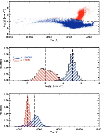
Figure 1.Top: KIC-based Surface Gravity–effective temperature H-R diagram of the stars in the analysis sample. The dashed black line marks the delineation to separate dwarfs (blue) and giants (red). Center: histograms of the surface gravity for the dwarfs (blue) and giants (red). The vertical dashed lines mark the median surface gravity values. Bottom: histograms of the effective temperatures for the dwarfs (blue) and giants (red). The vertical dashed lines mark the median temperature values.
and a truncated tail for the dwarf distribution of surface gravities; these artificial structures in the distributions indicated that the giant sample was significantly contaminated by dwarf stars at the 20% level. In an effort to transition more naturally between giants and dwarfs, we have employed a three-section (empirical) surface gravity cut determined from the surface gravity-effective temperature Hertzsprung–Russell (H-R) diagram (see Figure1). For three separate temperature ranges, a star was considered to be a dwarf if the surface gravity was greater than the value specified in the following algorithm:
log(g)
⎧ ⎨ ⎩
3.5 ifTeff 6000
4.0 ifTeff 4250
5.2−(2.8×10⁻⁴Teff) if 4250< Teff <6000.
The delineation between dwarfs and giants is shown in Figure1 by the dashed line with the dwarfs and giants high-lighted in blue and red, respectively.
The total number of stars separated into dwarfs and giants is 126,092 and 17,129, respectively. There is a clear separation in
The Astronomical Journal, 141:108 (21pp), 2011 April Ciardi et al.
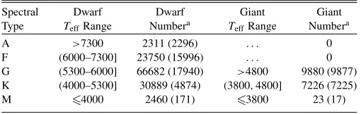
Figure 2.Temperature distributions (binsize=100 K) of the stars selected as dwarfs (top) and giants (bottom). The color coding illustrates the separation of the dwarfs and giants into temperature groups (i.e., spectral types).
Table 1
KIC-based Temperature Bins
Spectral Dwarf Dwarf Giant Giant
Type TeffRange Numbera TeffRange Numbera
A >7300 2311 (2296) . . . 0
F (6000–7300] 23750 (15996) . . . 0
G (5300–6000] 66682 (17940) >4800 9880 (9877)
K (4000–5300] 30889 (4874) (3800,4800] 7226 (7225)
M 4000 2460 (171) 3800 23 (17)
Note. a The number in parentheses is the number of stars brighter than Kepmag<14 mag.
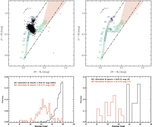
We have specifically explored the contamination rate of the M dwarfs with giant stars, by placing the M dwarfs on a Two Micron All Sky Survey (2MASS)JHKs color–color diagram, where the dwarf and giant colors are sufficiently different to enable separation (see Figure 4). Note that all of the M dwarfs, as identified from the KIC, have surface gravities of log(g)>4; yet, it is clear from the color–color diagram that a fraction of those identified as dwarfs are indeed giants. Using J−H =0.75 mag as the boundary between dwarfs and giants, we find that only ≈4% (108/2460) of the entire sample of stars identified as M dwarfs in the KIC actually have infrared
colors of giant stars. However, these contaminating stars are overwhelmingly brighter than the general M dwarf sample with 80% of the giant-color “dwarfs” having a Kepmag brighter than 13.5 mag (see Figure4). Thus, at the bright end of the M dwarf sample (Kepmag 13.5 mag), the giant contamination rate is50% (87/170). The inverse contamination is also evident. The entire M giant sample is much smaller with only 23 stars in total, but, of these, 6 (∼25%) haveJHKcolors of dwarfs. The contaminating M dwarfs are systematically fainter than the true M giants. For the sake of uniformity and continuity, we have not moved the contaminating sources into corresponding “correct” category; we do, however, exclude them when calculating the variability fractions.
3. VARIABILITY
For the spectral and luminosity classes defined above, we have assessed the distributions of the dispersion and variability to understand the broad stellar variability characteristics across the stellar spectrum. The analysis presented here utilized the statistics provided by NStED where the data were assessed using the native 30 minute sampling and the full 33 day time baseline of the data set. The time-series data are characterized by the dispersion about the median (σm) and by the reduced
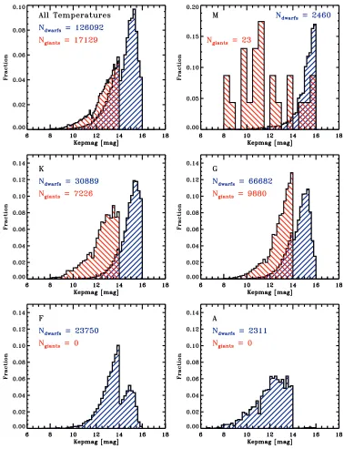
[image:4.612.42.297.499.580.2]Figure 3.Keplermagnitude distributions of the stars in the sample. Dwarfs and giants are represented by the blue- and red-hashed histograms, respectively. The panels represent the different temperature groups as labeled in the figures.
The first part of the study discusses the measured dispersions, and the second part of the study discusses the variability fractions of the stars within each group of stars. We also briefly explore the variability fraction of the stars as a function of the time baseline of the data set (1–33 days).
3.1. Photometric Dispersion
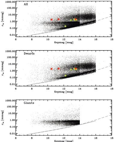
Figure5shows the 30 minute, 33 day photometric dispersion as a function ofKeplermagnitude for all the stars, separated out by dwarfs and giants, and Figure6displays the dispersions to the same scale, but separated by temperature as well. The gray dashed lines in Figures5and6correspond to the upper boundary on the uncertainties determined empirically for a constant background component (seeσupperin Jenkins et al.2010). The
gray solid line represents the median uncertainty value as a
function ofKeplermagnitude determined from the uncertainties provided with the data product as part of the light curves. To give some quantitative context to the number of stars within Figures5 and6, Table2tabulates the number of stars within four different ranges of dispersion. As instrumental precision plays a key role in the dispersion of the stars (particularly at the faint end), the stars are grouped not only by stellar class but also by magnitude range.
There are a few specific aspects to the dispersion diagrams that are worth noting. At fainter magnitudes (Kepmag 14 mag), the model uncertainties (gray solid and dashed lines in Figures5
The Astronomical Journal, 141:108 (21pp), 2011 April Ciardi et al.
Figure 4.Top: 2MASS color–color diagram for the stars identified as M dwarfs (left) and M giants (right) based upon the KIC surface gravities and effective temperatures. The green-hashed area marks the main sequence; the blue-hashed area marks the giant branch, and the red-hashed area marks the L dwarf locus. The diagonal lines mark the reddening zone for typical galactic interstellar extinction (R=3.1). Bottom: magnitude distributions for stars identified as dwarfs (left) and as giants (right) by their surface gravity. The black histograms are for stars with dwarf-likeJ−Hcolors; the red histograms are for stars with giant-likeJ−Hcolors. These plots show that the M stars brighter∼Kepmag<13.5 mag are predominately giants, regardless of their KIC classification.
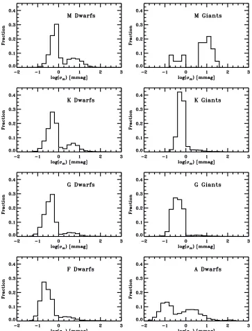
noise floor of the stars. This effect is most clearly seen in the giant stars where the Kepler data have sufficient preci-sion to detect the floor of the variability for the giant stars. The G and K giants occupy a very narrow range of photomet-ric dispersion between 0.1 and 1.0 mmag—completely inde-pendent of the magnitude. This narrow range of dispersion is most clearly apparent in the dispersion distribution histograms (Figure7).
The ubiquity of variability in giants has been noted previously (Gilliland2008) for a set of galactic bulge stars observed by the
Hubble Space Telescope (HST) over a time span of 7 days. Gilliland (2008) found that the typical amplitudes of variability were∼0.5 mmag for the G giants and increased to∼3.5 mmag for the late-K to early-M giants. We see a very similar trend in the dispersion which is most clearly demonstrated in Figure8
where we have plotted the photometric dispersion as a function of effective temperature. While there is a scattering of stars with large dispersions (and the number of M giants is very small), the giant stars occupy a very narrow region of variability that is
correlated with temperature. As expected from stellar evolution, the larger, cooler giants are more variable (e.g., Kjeldsen & Bedding1995) and the variability spans two orders of magnitude (0.1–10 mmag).
The dwarf stars are more complicated to interpret because their intrinsic dispersion is on the order of (or less than?) the photometric precision. Taken as a whole, they are more quiescent than the giant stars, as expected and demonstrated previously (Gilliland2008; Jenkins et al.2010; van Cleve2010; Basri et al.2010b), but there is a sample of stars at all magnitudes (Figure5) and all temperatures (Figures6–8) where the average dispersion is∼5 mmag. Histograms of the dispersion (Figure
7) and plotting the dispersion as a function of temperature (Figure8) highlight the bimodal dispersion, but show that only a relatively small percentage of stars are in the higher dispersion region.
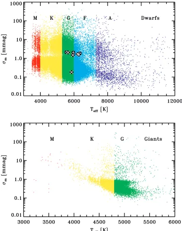
Figure 5.Photometric dispersion (30 minute sampling; 33 day timescale) of each star is plotted as a function of magnitude for all stars (top), for just the dwarfs (center), and for just the giants (bottom). In the top and center plots, the locations of the seven known planets in the sample are shown (red: BOKS-1, HAT-P-7, and TrES-2; green: Kepler-4,5,6,7,8). The gray line represents the median uncertainty as reported in theKeplerdata product. The dashed gray curve is the uncertainty upper limit curve from Jenkins et al. (2010).
NStED online periodogram service8 ∼ 90% of the inspected light curves displayed one or more significant periods (the ori-gin and distribution of the periods were not explored in this work). A similar visual inspection of 50 stars in the lower dis-persion region (but flagged as variable withχν2 >2) revealed that the variability was dominated by more stochastic “white noise” rather than periodic variability, and only∼25% of the stars displayed significant periodicity. It is also possible that these higher dispersions are an artifact of the data processing; however, this bimodal dispersion distribution (Figure7) for the dwarfs is also reported (although weaker) in Basri et al. (2010b) where they report a “variability excess” for those stars that are periodic versus those stars that are not periodic (Basri et al.
8 http://nsted.ipac.caltech.edu/applications/ETSS/kepler_index.html
2010b independently processed the data utilizing an empiri-cal polynomial fitting process). The details of the variability (e.g., periodic or stochastic, amplitude, and structure) have not been fully explored in the work presented here, but it should be noted that variability does not necessarily mean periodic behavior (Howell 2008) as all the stars in the visual inspec-tion were flagged as variable, but not all stars were (obviously) periodic.
The Astronomical Journal, 141:108 (21pp), 2011 April Ciardi et al.
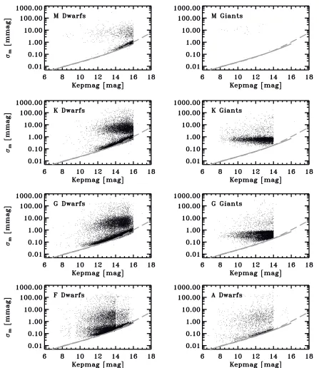
Figure 6.Photometric dispersion (30 minute sampling; 33 day timescale) of each star is plotted as a function of magnitude separated out by temperature and surface gravity as labeled in each panel. The solid gray line represents the median uncertainty value as reported in theKeplerdata product. The dashed gray curve is the uncertainty upper limit curve from Jenkins et al. (2010).
TrES-2, Kepler-4,5,6,7,8; Howell et al.2010; P´al et al.2008; O’Donovan et al.2006; Borucki et al.2010) on the dispersion diagrams (Figures5and8). The dispersions of the light curves in these systems are∼2 mmag, except for Kepler-4 where the light curve dispersion is ∼0.2 mmag. These light curves are nearly flat, to within the noise, except for the deep exoplanetary transits. If the transits are removed and the light curve statistics are recalculated, the dispersions decrease by almost an order magnitude for all the light curves except Kepler-4. All the planets (except Kepler-4) are Jupiter sized with transit depths of ∼1%, and it is the transits which dominate the statistics of the light curves. Kepler-4 is a much smaller (Neptune-sized) planet
with a transit depth of only∼0.1% which is comparable to the overall dispersion of the light curve.
3.2. Variability Fractions
The photometric dispersions (33 day baseline, 30 minute sampling) alone are not sufficient to assess the fraction of stars that are variable as the dispersion is dependent on the apparent magnitude of the targets, and, in particular, the dispersion for the dwarfs is at (or near) the precision limits of the instrument (for the 30 minute cadence). A more natural statistic is the reduced chi-square (χ2
ν) which takes into account the uncertainties (as
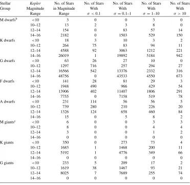
Table 2
Stars Separated by Class, Magnitude, and Dispersiona
Stellar Kepler No. of Stars No. of Stars No. of Stars No. of Stars No. of Stars
Group Magnitude in Magnitude With With With With
Range Range σ <0.1 σ=0.1–1 σ=1–10 σ >10
M dwarfsb <10 3 0 0 3 0
10–12 13 2 3 8 0
12–14 154 0 83 57 14
14–16 2182 0 1503 529 150
K dwarfs <10 18 3 10 3 2
10–12 264 75 83 94 11
12–14 4588 92 3063 1212 221
14–16 26019 1 19892 5184 942
G dwarfs <10 63 26 27 10 0
10–12 1297 716 257 294 27
12–14 16566 542 13376 2332 316
14–16 48756 0 43533 4550 673
F dwarfs <10 141 28 81 29 3
10–12 1948 490 966 429 54
12–14 13906 402 11407 1806 291
14–16 7755 0 7158 519 78
A dwarfs <10 231 114 56 56 5
10–12 739 280 210 226 20
12–14 1326 124 658 460 84
14–16 15 0 5 8 2
M giantsc <10 6 0 0 3 3
10–12 8 0 0 4 4
12–14 3 0 0 1 2
14–16 0 0 0 0 0
K giants <10 350 0 273 73 4
10–12 1683 1 1468 200 11
12–14 5192 1 4776 349 66
14–16 0 0 0 0 0
G giants <10 233 5 209 17 2
10–12 1619 38 1467 93 21
12–14 8025 7 7689 255 74
14–16 0 0 0 0 0
Notes.
aDispersions in millimagnitudes (mmag).
bThe 108 contaminating giants in the M dwarf sample have been removed from the statistics. cThe six contaminating dwarfs in the M giant sample have been removed from the statistics.
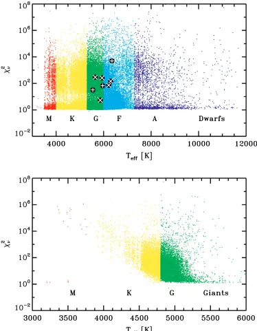
makes use of the provided point-to-point uncertainties in the light curves. For all light curves, the reduced chi-squares are calculated for the 33 day baseline (30 minute sampling) with respect to a constant median value and are plotted as a function of temperature (Figure9). For variability assessment purposes, a star is considered just-barely variable ifχ2
ν >2, significantly
variable ifχ2
ν >10, and very variable ifχν2 >100. Aχν2 ≈2
corresponds to an excess dispersion of approximately 1.5 times that of the measurement uncertainties; aχ2
ν ≈10 corresponds
to an excess dispersion of approximately three times that of the measurement uncertainties, and aχ2
ν ≈ 100 corresponds
to an excess dispersion of approximately 10 times that of the measurement uncertainties.
The measured fractions of stars that are variable are dependent upon the brightnesses of the stars as the instrumental precision decreases as the stars become fainter. Figure10plots the vari-ability fractions as a function of theKeplermagnitude for each of the stellar sub-groups. The magnitude bins are 0.5 mag in width, and the fractions were calculated for the three reduced chi-square categories listed above. Uncertainties on the fractions were calculated using standard error propagation (Everett et al.
2002). Some of the magnitude bins have very few stars
particu-larly at the bright end, and this is reflected in the relatively large error bars.
At the very bright end of the Kepler sample (Kepmag 11 mag), the variability fractions for the stars withχ2
ν >2 are
all near unity indicating that theKeplerprecision at 30 minute sampling is approaching the 33 day noise floor for the stars. Also for the brightest stars, the fractions of stars that are significantly variable (χ2
ν > 10) are 50%–100% depending on the
sub-group of stars. The fractions decrease as the stellar magnitude increases; this is, of course, a direct result of the decrease in the instrumental precision as the stars become fainter. Not surprisingly, at all brightnesses, the fractions of stars that are significantly variable (χ2
ν >10–100) are less than the fraction of
stars that are just-barely variable (χ2
ν >2). For the dwarfs, as the
stars grow fainter (Kepmag14 mag), the variability fractions are typically dominated by the extremely variable stars (χ2
ν >
The Astronomical Journal, 141:108 (21pp), 2011 April Ciardi et al.
Figure 7.Distributions of the (logarithmic) photometric dispersion (30 minute sampling; 33 day timescale) separated out by effective temperature and luminosity class as labeled in each panel.
as well as for 1 day and 10 day time baselines which are discussed in more detail in Section3.2.3.
3.2.1. The Dwarf Stars
The G dwarfs are the least variable group of dwarf stars with >80% of the stars being stable (Kepmag < 16 mag; χ2
ν <2); even with the magnitude restricted to the brightest stars
(Kepmag< 14 mag), the variability fraction of the G dwarfs is ∼30%. The floor for the G dwarf dispersion appears near 0.04 mmag (see Figure 6). The K dwarf and F dwarf stars have comparable variability fractions with≈50% of the stars identified as a variable if the magnitude is restricted to Kepmag<14 mag. The F dwarfs have a higher variability frac-tion if F dwarfs of all magnitudes are considered, but this is a result of the different magnitude distributions of the K and F dwarfs in the sample (see Figure3). The relative number of F
and K stars brighter than and fainter than Kepmag ≈ 14 mag differ, with the K dwarfs having significantly more fainter stars than brighter stars. The differing magnitude distributions for the F and K dwarfs are a result of the target selection criteria optimized for searching for transiting planets around as many appropriate stars as possible (Batalha et al.2010).
Figure 8.Photometric dispersion (30 minute sampling; 33 day timescale) of each star is plotted as a function of effective temperature separated out by temperature (colors and labels) and surface gravity (top and bottom panels). The black points in the top panel mark the locations of the seven known planets in the sample (+: BOKS-1, HAT-P-7, and TrES-2;×: Kepler-4,5,6,7,8).
fraction of variable A stars is likely the result of the A star group (as identified from the KIC) including stars in the instability regime, suchγDor,δScu, slowly pulsating B stars (SPBs), RR Lyr, andβ Cep stars.Hipparcosfound the variability fractions of these sub-groups to range from 10% to 100%.
3.2.2. The Giant Stars
At the precision of Kepler, nearly all of the giants are variable, with 94%, 99%, and 100% variability fractions (33 day baseline, 30 minute sampling) for the G, K, and M giants, respectively. The six M stars with dwarfJ−Hcolors have been removed from the statistics. The G giants variability fraction is slightly reduced by the faint end of the brightness distribution, where the stability floor approaches the instrument limit for Kepmag≈14 mag, but only because the stability floor of the G giants is 0.1 mmag versus 0.3 mmag for the K giants. For the M
giants, the dispersion and stability floor is substantially higher at levels of∼10 mmag.
The Astronomical Journal, 141:108 (21pp), 2011 April Ciardi et al.
Figure 9.Photometric reduced chi-square (30 minute sampling; 33 day timescale) of each star is plotted as a function of effective temperature separated out by temperature (colors and labels) and surface gravity (top and bottom panels). The black points in the top panel mark the locations of the seven known planets in the sample (+: BOKS-1, HAT-P-7, and TrES-2;×: Kepler-4,5,6,7,8).
Assuming that the photometric dispersion in theKeplergiants is also dominated by acoustic oscillations, the photometric variations can be used to predict radial velocity amplitudes of the oscillations. Kjeldsen & Bedding (1995) developed a calibrated relationship between the velocity of oscillations and the photometric amplitude variations:
σrv=
(F /F)λ
20.1×10⁻⁶
λ 0.55μm
Teff
5777 2
m s−1,
whereσrvis the oscillation velocity of the star,(F /F)λis the
photometric flux change at the observed wavelengthλ, andTeff
is the effective temperature of the star. Using this relation, we have calculated the expected radial velocity oscillations for the
G and K giants based upon their photometric dispersions and effective temperatures (see Figure11).
The bulk of predicted radial velocity dispersions are cen-tered around 10–20 m s−1with 90% of the velocities30 m s−1. The K giants have a symmetric distribution centered at σrv ≈ 20±5 m s−1. This is in good agreement with a
Figure 10.Variability fractions of stars as a function of the brightness (Keplermagnitude). The contaminating giants in the M dwarf sample and the contaminating dwarfs in the M giant sample have been removed from the statistics. The blue curves represent the fractions of stars withχ2
The Astronomical Journal, 141:108 (21pp), 2011 April Ciardi et al.
Table 3 Variability Fractionsa
Time χν2>2 χν2>10 χν2>100
Scale Category 16 mag 14 mag 16 mag 14 mag 16 mag 14 mag
33 day All dwarfs 0.269 (0.002) 0.461 (0.004) 0.177 (0.001) 0.269 (0.003) 0.123 (0.001) 0.200 (0.002) M dwarfsb 0.367 (0.014) 0.690 (0.083) 0.285 (0.012) 0.497 (0.065) 0.209 (0.010) 0.474 (0.064) K dwarfs 0.298 (0.004) 0.532 (0.013) 0.224 (0.003) 0.347 (0.010) 0.161 (0.002) 0.316 (0.009) G dwarfs 0.183 (0.002) 0.325 (0.005) 0.125 (0.002) 0.199 (0.004) 0.090 (0.001) 0.164 (0.003) F dwarfs 0.421 (0.005) 0.555 (0.007) 0.212 (0.003) 0.279 (0.005) 0.127 (0.003) 0.169 (0.004) A dwarfs 0.705 (0.023) 0.705 (0.023) 0.559 (0.019) 0.558 (0.019) 0.434 (0.016) 0.435 (0.016) All giants 0.962 (0.011) 0.962 (0.011) 0.717 (0.009) 0.717 (0.008) 0.210 (0.004) 0.210 (0.004) M giantsc 1.000 (0.343) 1.000 (0.343) 1.000 (0.343) 1.000 (0.343) 1.000 (0.343) 1.000 (0.343) K giants 0.996 (0.017) 0.996 (0.017) 0.886 (0.015) 0.886 (0.015) 0.314 (0.008) 0.314 (0.008) G giants 0.938 (0.014) 0.938 (0.014) 0.593 (0.010) 0.593 (0.010) 0.135 (0.004) 0.135 (0.004) 10 day All dwarfs 0.268 (0.002) 0.461 (0.004) 0.167 (0.001) 0.260 (0.003) 0.097 (0.001) 0.167 (0.002) M dwarfsb 0.367 (0.014) 0.678 (0.082) 0.269 (0.012) 0.474 (0.063) 0.163 (0.009) 0.404 (0.058) K dwarfs 0.299 (0.004) 0.535 (0.013) 0.212 (0.003) 0.341 (0.010) 0.127 (0.002) 0.275 (0.008) G dwarfs 0.182 (0.002) 0.328 (0.005) 0.117 (0.001) 0.189 (0.004) 0.069 (0.001) 0.128 (0.003) F dwarfs 0.417 (0.005) 0.551 (0.007) 0.205 (0.003) 0.272 (0.005) 0.102 (0.002) 0.141 (0.003) A dwarfs 0.690 (0.022) 0.689 (0.023) 0.548 (0.019) 0.548 (0.019) 0.417 (0.016) 0.417 (0.016) All giants 0.961 (0.011) 0.962 (0.011) 0.713 (0.009) 0.713 (0.008) 0.202 (0.004) 0.202 (0.004) M giantsc 1.000 (0.343) 1.000 (0.343) 1.000 (0.343) 1.000 (0.343) 1.000 (0.343) 1.000 (0.343) K giants 0.995 (0.017) 0.995 (0.017) 0.883 (0.015) 0.838 (0.015) 0.303 (0.007) 0.304 (0.007) G giants 0.937 (0.014) 0.937 (0.014) 0.589 (0.010) 0.589 (0.010) 0.128 (0.004) 0.128 (0.004) 1 day All dwarfs 0.264 (0.002) 0.432 (0.004) 0.089 (0.001) 0.183 (0.002) 0.042 (0.001) 0.097 (0.002) M dwarfsb 0.320 (0.013) 0.567 (0.072) 0.128 (0.008) 0.281 (0.046) 0.077 (0.006) 0.152 (0.032) K dwarfs 0.279 (0.003) 0.491 (0.012) 0.082 (0.002) 0.205 (0.007) 0.033 (0.001) 0.093 (0.005) G dwarfs 0.193 (0.002) 0.312 (0.005) 0.054 (0.001) 0.105 (0.003) 0.021 (0.001) 0.050 (0.002) F dwarfs 0.397 (0.005) 0.513 (0.007) 0.152 (0.003) 0.211 (0.004) 0.077 (0.002) 0.108 (0.003) A dwarfs 0.678 (0.022) 0.679 (0.022) 0.519 (0.018) 0.520 (0.019) 0.389 (0.015) 0.340 (0.015) All giants 0.955 (0.010) 0.955 (0.010) 0.668 (0.008) 0.668 (0.008) 0.174 (0.003) 0.174 (0.003) M giantsc 1.000 (0.343) 1.000 (0.343) 1.000 (0.343) 1.000 (0.343) 0.941 (0.323) 0.941 (0.328) K giants 0.995 (0.017) 0.995 (0.017) 0.839 (0.015) 0.838 (0.015) 0.266 (0.007) 0.266 (0.007) G giants 0.925 (0.013) 0.925 (0.013) 0.544 (0.009) 0.544 (0.009) 0.107 (0.003) 0.107 (0.003)
Notes.
aValues in parentheses are uncertainties based upon the propagation of errors of the counting statistics. bThe 108 contaminating giants in the M dwarf sample have been removed from the statistics. cThe six contaminating dwarfs in the M giant sample have been removed from the statistics.
The G giants predicted velocities show a bimodal structure with peaks near 10 and 20 m s−1with the stronger peak toward lower radial velocity variations. The magnitude distributions of the G giants that have predicted radial velocity amplitudes of <15 m s−1 and those that have predicted radial velocity amplitudes of>15 m s−1 are indistinguishable indicating that the bimodality is not related to the brightness (and hence, the photometric precision) of the stars, but rather is intrinsic to the sample. The radial velocity appears uncorrelated with temperature, but does appear to have a weak anti-correlation with surface gravity,9 suggesting that the G giant sample may contain a sampling of dwarfs and sub-giants, which are atmospherically more stable than the G giants.
3.2.3. Time-dependent Variability
The analysis, thus far, has been performed on the full 33.5 day time baseline of the quarter-1 data set (30 minute cadence), but in reality, stars are variable on a variety of timescales depending on the source of the variability (e.g., flares, pulsations, rotation, and eclipses; Eyer & Mowlavi2008). A full detailed study of
9 The Kendall-τnon-parametric rank correlation value between the surface gravities and the predicted radial velocity oscillations is−0.75 (number of standard deviations from zero is≈100); a value of−1 would indicate a perfect anti-correlation.
Figure 11.Distribution of radial velocity oscillations of G (blue) and K (red) giants predicted from the photometric dispersion and effective temperature (Kjeldsen & Bedding1995). The dashed line marks the median radial velocity oscillation for the K giant sample of Frink et al. (2001).
[image:14.612.332.551.472.630.2]Figure 12.Variability fraction distributions as a function of sampling. Each panel represents a different group of stars. There are two panels for each group; one panel for all the stars in the sample and one panel where the stars were restricted to aKeplermagnitude of 14 or brighter. The contaminating giants in the M dwarf sample and the contaminating dwarfs in the M giant sample have been removed from the statistics. The blue curves represent the fractions of stars withχ2
ν >2; the green curves represent the fractions of stars withχ2
The Astronomical Journal, 141:108 (21pp), 2011 April Ciardi et al.
Figure 13.Galactic coordinates plot of the positions of all the stars in the sample. The red box delineates the 10◦×10◦region used to explore the variability as a function of galactic latitude.
long-term variability or enhance some forms of variability (van Cleve2010), and the detailed results of this short study should be viewed with that in mind.
For each of the light curves, we have assessed the light curve properties with progressively longer time baselines starting at 1 day and extending to 33 days. The median, the dispersion about the median, and the reduced chi-square assuming a constant median value were calculated for each time interval. To help alleviate biases that might arise from sampling the light curves in progressively longer samples in a single direction, the statistics were calculated by sampling the light curves in the time-forward direction (0–1 day, 0–2 day 0–3 day, . . . 0–33 day) and in the time-backward direction (33–32 day, 33–31 day 33–30 day, . . .33–0 day) and the results were averaged. In Table 3 and Figure 12, the dependency of the derived variability fractions is summarized. As with the overall variability statistics, the analysis was performed for all stars (Kepmag < 16 mag) and for the brighter end of the sample (Kepmag<14 mag).
The overall fractions of giants that are variable (χ2
ν >2) do
not change to within the uncertainties of the fractions as the time baseline is increased from 1 day to 33 days. The fraction of giant stars that are more significantly variable (χ2
ν >10 and
χν2 > 100) does grow by ≈4%–5% from the 1 day baseline to the 33 day baseline. The small growth of the variability fractions is likely a result of the fact that nearly all of the giants are observed to be variable at the precision ofKeplerand the variability fraction has little room to change.
For the dwarf stars, the overall variability fractions (χν2>2) increase by≈1%–5%, as the baseline is increased to 33 days. As with the giants, the variability fraction changes more sub-stantially for those stars that are more significantly variable (χ2
ν >10 andχν2 >100). Larger amplitude variability
requir-ing longer time periods is not surprisrequir-ing and has been observed previously (e.g., Eyer & Mowlavi2008). Increasing the time baseline from 1 day to 33 days increases the variability frac-tions for the M dwarf, K dwarf, and G dwarf stars variability more than for the F dwarf and A dwarf stars. This suggests that
Table 4 Galactic Distributions
Category Median Median Typical Scale Fraction of
Teff Kepmag Distance Heightz◦ Stars
(K) (mag) (pc) (pc)a z2.3z
◦
M dwarfs 3800 15.3 200 35 0.97
K dwarfs 5000 15.1 600 75 0.68
G dwarfs 5700 14.7 1000 105 0.56
F dwarfs 6200 13.6 1100 185 0.83
A dwarfs 8000 12.3 1200 165 0.77
G giants 5000 13.1 2800 235 0.40
K giants 4700 12.7 2500 215 0.43
Note.aCalculated by fitting thez-height distributions in Figure14.
the lower mass stars are predominately characterized by vari-ability with timescales of weeks (e.g., rotational modulation) while the higher mass stars are predominately characterized by variability with timescales of days (e.g., pulsations).
3.3. Galactic Distribution
TheKeplerfield spans approximately 12◦in galactic latitude (b≈8◦–20◦). Over this range of latitude, the different galactic populations may play a role in the variability fractions. Because the target samples are mostly magnitude limited, the differing intrinsic brightnesses of the stars lead to differing median distances of the stars for each sub-group, and hence, to differing median heights (z) above the galactic plane for a given line of sight. Walkowicz et al. (2011) found a higher fraction of the flaring M and K dwarfs at lowerz-heights, and they suggested that they were sampling primarily the young thin disk. Their work inspired us to try to understand the overall variability fraction of the sample as a function of latitude andz-height for each of the stellar sub-groups.
A subset of the Kepler field was selected (see Figure 13) to remove the effects of the rotation of the Kepler field with respect to the Galactic plane. The median temperature and magnitude for each category of stars was used to determine a “typical” distance for the stars, assuming zero attenuation by interstellar dust (see Table 4). The z-height of each star was computed from the typical distance for its sub-group, its apparent magnitude, and its galactic latitude. This simple estimation assumes that each star within a sub-group has the same absolute magnitude. While this, of course, is not strictly correct, the typical spread of absolute magnitude within a sub-group is ≈1–2 mag, corresponding to only a factor of 1.2–1.5 in the distance. Thez-height distributions of the stars (Figure14) mostly follow the expected exponential decay for a disk of the formN ∝exp(−z/z◦),wherez◦is the characteristic scale height of the disk (Ciardi et al.1996; Juri´c et al.2008). Eachz-height distribution was fitted with a decaying exponential and the resulting scale heights are listed in Table 4. The exponential fits work best for the intrinsically brightest stars (e.g., the F dwarfs, A dwarfs, K giants, and G giants) where local distribution effects are minimized.
[image:16.612.316.570.75.185.2]Figure 14.z-height distributions for the dwarfs and G and K giants. The black smooth curves represent the best-fit exponential curves to the distributions. The M giants have been excluded from the plot because of the low number (23) in the sample.
from only this one disk population, it is expected that∼90% of the stars will havez-heights withinz 2.3z◦. The actual fractions are listed in Table 4; all of which are significantly below 90%, indicating that the thick disk may contribute to the overall sample—particularly at higher galactic latitudes. The thick disk has a scale height of≈900 pc and a scaling fraction of∼10% (Juri´c et al.2008).
If the thin disk contributes only a portion (albeit the majority fraction) to the sample of stars observed byKepler, a variation in the variability fraction as a function of galactic latitude (i.e., scale height) might be expected. Figure15displays the fraction of stable stars (χ2
ν <2) and variable stars (χν2>2) as a function
of galactic latitude for each of the sub-groups (K giants and M giants are not included in this sample as “all” of the K giants are variable at the precision ofKepler). The M, K, G, and F dwarfs all show an increase in the variability fraction as the galactic
latitude gets lower (i.e., closer to the plane). Moving higher in galactic latitude, the variability fractions decrease by ∼0.1% over the 10◦span of theKeplerfield. This could indeed be the result of sampling younger stars in the plane at lower latitudes as young stars are expected to be more active (West et al.2008). Indeed, the flaring rate of M dwarfs as a function of z-height suggests that stars located nearer to the galactic plane are more active and, hence, more variable (Walkowicz et al. 2011) in reasonable agreement with what is discussed here.
The Astronomical Journal, 141:108 (21pp), 2011 April Ciardi et al.
Figure 15.Galactic latitude distributions (binsize=1◦) for the dwarfs and G giants. The black curves represent the fraction of stars within that galactic latitude bin that are deemed “stable” (χ2
ν <2), and the red curves represent the fraction of those stars that are deemed “variable” (χν2>2). The black dashed line is a best fit to the variability fraction as a function of galactic latitude with the parameters of the line fit given in each panel.
and F dwarfs), and is not apparent for the most intrinsically bright stars (A dwarfs and G giants). As theKeplersample is magnitude limited with similar magnitude ranges for each of the stellar sub-groups, the different sub-groups are essentially sampling different distances (see Table4).
For the thin disk (z◦∼300 pc), the path length to outside the disk (z∼600 pc) is≈4300 pc atb∼8◦, but only≈1750 pc at b∼20◦. For the M dwarfs with typical distances of 200 pc, the latitude change corresponds to a background path length (for a conic volume) difference of nearly 40% from low (b ∼ 8◦) to high (b ∼20◦) galactic latitude. For the G, F, and A dwarfs (d∼1000 pc), the background volume difference is20%. The reduction in background path length is approximately 50% from
M dwarfs to F dwarfs, which is also the fraction by which the slopes of the variability fraction versus latitude change from M dwarfs to G and F dwarfs (see Figure15). The A dwarfs do not display a reduction in the variability fraction at higher latitudes; if anything, they exhibit a weak (and somewhat insignificant) increase in variability at higher latitudes. The G giant stars, with typical distances that are larger than the line-of-sight distances to the “top” of the exponential disk atb ∼10◦–20◦, show no dependence of the variability fraction on the galactic latitude. All of this is consistent with background stars contributing to the variability of the primary stars.
Without a full model of the stellar galactic distribution
Figure 16.2MASS color–color diagram for the 29 stars identified as M dwarfs from outside catalogs.
of the relative populations, it is difficult to disentangle these scenarios (true variability fractional changes as a function of latitude versus changes in the background contamination rate). However, the apparent correlation of flare rates with lower z-height (Walkowicz et al.2011) does suggest that the higher variability fraction at lower galactic latitudes may be real and the result of sampling a systematic younger population.
3.4. M Dwarf Variability
M dwarfs are favorable targets to search for Earth-sized plan-ets because the transits are relatively deep (∼1–3 mmag), and the radial velocity signatures are relatively large (∼10 m s−1). In addition, planets in the habitable zones of m stars are in rela-tively short orbits (10–20 days) compared to that of the habitable zones for Sun-like stars (∼1 yr). As a result there has been a strong interest in the community for searching for planets around M stars (Irwin et al.2009; Charbonneau et al.2009; Bean et al.
2010). Thus, characterizing the M dwarf variability amplitudes and fractions is critical for a better understanding of the com-pleteness of transit and radial velocity surveys geared toward M dwarfs.
In the previous sections (Sections3.1 and3.2), the overall variability fraction of the M dwarfs was found to be∼40%–70% with dispersions of σm ∼ 3–5 mmag, depending on the
brightness of the stars being considered. As an alternative, in this section we identify a small sample of relatively bright, certain M dwarfs based on well-vetted proper motion catalogs and analyze their variability in more detail. These M dwarfs include all of the M dwarfs in theKeplerfield (with Q1 light curves) from the Gliese and LHS catalogs (Stauffer et al.2010) and the brightest stars in the LSPM catalog withV −J >2.6 (i.e., colors consistent with an M dwarf). A plot ofJ−Hversus
Table 5 M Dwarf Stars
Star KIC KIC KIC σm σm
Name ID Teff log(g) 33 day 12 hr
(K) (cm s−2) (mmag) (mmag)
LHS6351 2164791 . . . . . . 6.09 1.69
LSP1912+3826 3330684 . . . . . . 0.42 0.41
LSP1909+3910 4043389 3713 4.385 7.94 0.17
GJ4099 4142913 . . . . . . 4.05 0.10
GJ4113 4470937 . . . . . . 0.06 0.04
LSP1917+4007 5002836 . . . . . . 0.10 0.10
LSP1947+4020 5206997 . . . . . . 2.93 0.13
LSP1935+4119 6049470 . . . . . . 2.05 0.09
LSP1919+4127 6117602 . . . . . . 3.84 2.13
LSP1858+4147 6345835 . . . . . . 2.84 0.08
LSP1956+4149 6471285 3201 0.07 0.20 0.18
LSP1927+4231 7033670 . . . . . . 0.36 0.28
LSP1944+4232 7049465 4033 4.505 1.47 0.08
LSP1912+4239 7106807 . . . . . . 0.12 0.11
LSP1912+4316 7596910 . . . . . . 0.20 0.19
LHS6349 7820535 . . . . . . 0.34 0.33
LSP1854+4447 8607728 . . . . . . 7.06 0.31
LSP2001+4500 8846163 . . . . . . 0.17 0.15
LHS3429 8872565 . . . . . . 0.12 0.11
LSP1933+4515 8957023 3553 4.117 7.82 0.18
LHS3420 9201463 . . . . . . 39.8 7.13
GJ1243 9726699 . . . . . . 11.6 9.69
LHS6343 10002261 . . . . . . 3.07 0.68
LSP1857+4720 10258179 . . . . . . 0.11 0.10
LSP1854+4736 10453314 . . . . . . 0.17 0.14
GJ4083 10647081 . . . . . . 4.69 0.08
LSP1916+4949 11707868 . . . . . . 0.11 0.14
LSP1948+5015 11925804 . . . . . . 0.79 0.55
[image:19.612.316.568.407.747.2]The Astronomical Journal, 141:108 (21pp), 2011 April Ciardi et al.
Figure 17.Left panels show the photometric dispersion plotted as a function of magnitude for the KIC-identified M dwarfs with a color restriction ofJ−H<0.75 mag (black dots) and for the outside identified M dwarfs (red). The solid gray line represents the median uncertainty as reported in theKeplerdata product. The dashed gray curve is the uncertainty upper limit curve from Jenkins et al. (2010). Right panels show the distributions of the (logarithmic) photometric dispersion (binsize=0.2 dex) for the known M dwarfs (red points in left panels). The top panels reflect the dispersion of the known M dwarfs determined for the entire light curve (30 days); the bottom panels reflect the dispersion calculated from the point-to-point differences on 12 hr timescales (only for the known (red points) M dwarfs). The KIC-identified M dwarfs (black dots) are shown at the 30 minute cadence dispersion in both plots for reference.
H−K confirms that these are indeed M dwarfs (Figure 16). Only four of these stars have KICTeffor log(g)—the rest would
be absent from statistical studies which rely onTeff and log(g)
to identify dwarfs, and, of these, one would have been classified as a giant.
To understand the variability of these bright M dwarfs on the timescales relevant to planetary transits, we have calculated the short-term 12 hr variability for each of the light curves by computing the dispersions in running 12 hr time bins. The median of all the 12 hr bin dispersions for each light curve was calculated and taken as representative of the 12 hr variability timescales for the M dwarfs. The dispersions for the full time series (33 days) and for the 12 hr timescales are listed in Table 5. In all cases, the dispersion on the 12 hr timescale is smaller than the full 30 day dispersion, and for many of the stars, the dispersion drops to the photometric limit of instrument (see Figure17).
On the 33 day timescale, the dispersion is bimodal with peaks near 0.1 mmag and 5 mmag. The 0.1 mmag peak is dominated by stars which are quiet to the precision of the instrument, and ≈1/2 (15/29) of the sample are variable with χ2
ν > 2
and dispersions of σm 1 mmag. For the 12 hr timescale,
the variability fraction drops significantly with only six stars that have dispersions σm > 0.5 mmag. The high dispersion
is likely caused by rotational variability with periods of 1 day or longer; thus, it is not all that surprising that the dispersion drops when the light curves are sampled at 12 hr timescales. A prime example of this is LHS6343 (KIC 10002261) which is a newly discovered transiting brown dwarf (Johnson et al.2010). The dispersion for the entire light curve is ≈3 mmag, but the 12 hr timescale dispersion matches the out-of-eclipse dispersion of≈0.7 mmag—much like what is observed for the transiting planets around FGK stars (see Section3.1).
4. SUMMARY
An analysis of the variability statistics of the stars in the quarter-1 publicly released Kepler data has been performed. TheKeplerdata cover 33.5 days and are sampled at a 30 minute cadence. The KIC parameters have been used to separate the 150,000 stars into dwarfs and giants which were further sepa-rated into temperature bins corresponding roughly to spectral classes A, F, G, K, and M.
of theKeplerspacecraft. The derived variability fractions range from 10% to 100% depending on the stellar group and bright-ness range explored. The G dwarfs are the most stable with <20% of the all the stars in the sample having aχ2
ν 2. The G
dwarfs appear to have a dispersion noise floor of∼0.04 mmag for the 30 minute sampling of theKeplerdata.
At the precision ofKepler,>95% of K, G, and M giants are variable with noise floors of∼0.1 mmag,∼0.3 mmag, and∼10 mmag, respectively. The photometric dispersion of the giants is consistent with acoustic variations of the photosphere. The photometrically predicted radial velocity distribution for the K giants is in agreement with the measured distribution; the G giant radial velocity distribution is bimodal which may indicate a transition from sub-giant to giant.
We also briefly explored the dependence of the variability fractions as a function of time baseline of the light curves. In general, increasing the length of the light curve baseline increased the fraction of stars that are variable. For the dwarf stars, the lower mass stars were found to be predominately characterized by variability with timescales of weeks (e.g., rotational modulation) while the higher mass stars were found to be predominately characterized by variability with timescales of days (e.g., pulsations). For the giant stars, the variability fractions changed very little from a 1 day sampling to a 33 day sampling.
A study of the distribution of the variability as a function of galactic latitude suggests that sources closer to the galactic plane are more variable. The scale height distribution of the dwarfs is consistent with the young thin disk, and the scale height of the giants is consistent with the older thin disk. For the lower mass stars (M, K, and G dwarfs), the variability fraction decreases with increasing galactic latitude. This may be the result of sampling differing populations as a function of latitude and preferentially sampling younger stars at lower galactic latitudes within theKeplerfield.
In addition to the statistical study of M dwarf variability using the 2500 relatively anonymous probable M dwarfs in theKepler
field, we have also examined the variability of 29 known M dwarfs in theKeplerfield drawn from the GJ, LHS, and LSPM catalogs. The analysis of the known M dwarfs indicates that the M dwarfs are primarily variable on timescales of weeks presumably dominated by spots, rotation, and binarity. But on shorter timescales of hours to days, the stars are quieter by nearly an order of magnitude. At these shorter timescales, the variability fraction of the M dwarfs drops from∼40% to∼20%. The shorter timescales are relevant for searches of planetary transits which typically last a few hours. In general, a search for transiting Earth-sized planets around M stars should not be hampered by the typical stellar variability of M dwarfs.
The authors acknowledge the referee for his or her extremely insightful and useful comments which made this a better paper. Portions of this work were performed at the California Institute of Technology under contract with the National Aeronautics and Space Administration. This research has made use of the NASA/IPAC Star and Exoplanet Database, which is operated by the Jet Propulsion Laboratory, California Institute of Tech-nology, under contract with the National Aeronautics and Space Administration.
REFERENCES
Auvergne, M., et al. 2009,A&A,506, 411 Basri, G., et al. 2010,ApJ,713, L155 Basri, G., et al. 2011,AJ,141, 20 Batalha, N., et al. 2010,ApJ,713, L109 Bean, J. L., et al. 2010,ApJ,713, 410 Borucki, W. J., et al. 2010,Science,327, 977 Charbonneau, D., et al. 2009,Nature,462, 891 Ciardi, D. R., et al. 1996,AJ,112, 700
Drilling, J. S., & Landolt, A. U. 2000, in Allen’s Astrophysical Quantities, ed. A. N. Cox (4th ed.; New York: AIP),381
Everett, M. E., Howell, S. B., van Belle, G. T., & Ciardi, D. R. 2002,PASP, 114, 656
Eyer, L., & Grenon, M. 1997, in Hipparcos: Venice 97, ed. B. Battrick (ESA SP-402; Noordwijk: ESA),467
Eyer, L., & Mowlavi, N. 2008,J. Phys. Conf. Ser.,118, 012010 Frink, S., et al. 2001,PASP,113, 173
Gilliland, R. L. 2008,AJ,136, 566 Hartman, J. D., et al. 2004,AJ,128, 1761 Henry, G. W., et al. 2000,ApJS,130, 201 Howell, S. B. 2008,Astron. Nachr.,329, 259 Howell, S. B., et al. 2010,ApJ,725, 1633
Huber, M. E., Everett, M. E., & Howell, S. B. 2006,AJ,132, 633
Irwin, J., Charbonneau, D., Nutzman, P., & Falco, E. 2009, in IAU Symp. 253, Transiting Planets (Cambridge: Cambridge Univ. Press),37
Jenkins, J. M., et al. 2010,ApJ,713, L120 Johnson, H. L. 1966,ARA&A,4, 193
Johnson, J. A., et al. 2010, ApJ, arXiv:1008.4141 Juri´c, M., et al. 2008,ApJ,673, 864
Kane, S. R., et al. 2005,MNRAS,362, 117 Kjeldsen, H., & Bedding, T. R. 1995, A&A,293, 87 Koch, D. G., et al. 2010,ApJ,713, L79
Latham, D. W., et al. 2005, BAAS,37, 1340
Majewski, S. R., Ostheimer, J. C., Kunkel, W. E., & Patterson, R. J. 2000,AJ, 120, 2550
Matthews, J., et al. 1999, J. R. Astron. Soc. Can.,93, 183 O’Donovan, F. T., et al. 2006,ApJ,651, L61
P´al, A., et al. 2008,ApJ,680, 1450
Pickering, E. C. 1881,Proc. Am. Acad. Arts Sci., 16, 257 Pojmanski, G. 2002, Acta Astron.,52, 397
Stauffer, J., et al. 2010,PASP,122, 885
van Cleve, J. 2010, Kepler Data Release 6 Notes, KSCI-19046-001 Walkowicz, L. M., et al. 2011,AJ,141, 50
West, A. A., et al. 2008,AJ,135, 785