A probabilistic framework for online structural health monitoring : active learning from machining data streams

http://eprints.whiterose.ac.uk/152299/

Version: Published Version

Proceedings Paper:

Bull, L.A., Worden, K. orcid.org/0000-0002-1035-238X, Rogers, T.J.

orcid.org/0000-0002-3433-3247 et al. (5 more authors) (2019) A probabilistic framework for

online structural health monitoring : active learning from machining data streams. In:

Journal of Physics: Conference Series. Thirteenth International Conference on Recent

Advances in Structural Dynamics (RASD), 15-17 Apr 2019, Valpre, Lyon, France. IOP

Publishing .

https://doi.org/10.1088/1742-6596/1264/1/012028

[email protected] https://eprints.whiterose.ac.uk/

Reuse

This article is distributed under the terms of the Creative Commons Attribution (CC BY) licence. This licence allows you to distribute, remix, tweak, and build upon the work, even commercially, as long as you credit the authors for the original work. More information and the full terms of the licence here:

https://creativecommons.org/licenses/ Takedown

If you consider content in White Rose Research Online to be in breach of UK law, please notify us by

PAPER • OPEN ACCESS

A probabilistic framework for online structural health monitoring: active

learning from machining data streams

To cite this article: L A Bull et al 2019 J. Phys.: Conf. Ser. 1264 012028

Content from this work may be used under the terms of theCreative Commons Attribution 3.0 licence. Any further distribution of this work must maintain attribution to the author(s) and the title of the work, journal citation and DOI.

Published under licence by IOP Publishing Ltd 1

A probabilistic framework for online structural

health monitoring: active learning from machining

data streams

L A Bull1, K Worden1, T J Rogers1, C Wickramarachchi1, E J Cross1, T McLeay2, W Leahy3 and N Dervilis1

1

Dynamics Research Group, Department of Mechanical Engineering, The University of Sheffield, Mapping Building, Mappin Street, Sheffield, S1 3JD.

2

Advanced Manufacturing Research Centre, Advanced Manufacturing Park, Wallis Way, Catcliffe, Rotherham S60 5TZ

3

Element Six Global Innovation Centre, Harwell Campus, Fermi Ave, Didcot OX11 0QR

E-mail: [email protected]

Abstract. A critical issue for data-based engineering is a lack of descriptive labels for the measured data. For many engineering systems, these labels are costly and/or impractical to obtain, and as a result, conventional supervised learning is not feasible. This paper suggests a probabilistic framework for the investigation and labelling of engineering datasets; specifically, acoustic emission data streams recorded online from a turning machine. Two alternative probabilistic measures are suggested to select the most informative observations. During machining operations, these data would then be investigated and annotated by an engineer, in order to maximise the classification performance of a statistical model used to predict tool wear.

1. Introduction

Advanced structural health monitoring (SHM) systems look to provide a framework for the classification and localisation of damage, following preliminary damage detection. This framework requires the categorisation of many data-groups, i.e. classes, relating to different states of structural health — rather than simply classifying data as either normal or novel (outlier analysis) [1, 2]. In an engineering context, a critical issue for the multi-class problem is a lack of comprehensive labelled data, which are required to learn a (standard) supervised classification algorithm. Furthermore, in an online setting for SHM, the measured data arrive as a stream, incrementally, throughout the lifetime of the monitored structure.

outlines an approach to address the investigation of engineering data streams in a semi-supervised, probabilistic framework for online SHM.

2. Semi-supervised learning for structural health monitoring

Classifying measured data via a robust model (learnt from a limited subset of training data) is a fundamental problem in the field of engineering pattern recognition. Generally, the measured data, x_{i ∈X, can be categorised according to descriptive labels, yi ∈Y, which correspond to}

the ground truth of the classification problem. From a probabilistic perspective, it is assumed that X is a random vector, defining a D-dimensional feature space, such that X ∈ RD. The descriptive labels are defined by a discrete random variable, such that yi ∈Y ={1, ..., K}; here

K is the number of classes, andY denotes the label space.

Supervised pattern-recognition algorithms require fully labelled training-data,L_{, such that} [3],

L_={(x_{i, yi)|}x_{i ∈X, yi ∈Y}}n

i=1, (1)

for ncollected data points. As the training set, L_{, includes both measured data and descriptive} labels, a supervised classifier can learn a mapping between the feature space and the label space,

f :X→Y. The classifier, f, can then be used to predict the label of future measurements, and thus, make diagnostic decisions in an SHM context. In contrast, unsupervised techniques are applied when only the measured data are available to build a model. In this case, the training-set becomes [3],

U_={x_ˆi|x_{ˆi ∈X}}m

i=1. (2)

The caret is used to denote measured data that are unlabelled. A variety of machine learning tools can be applied to unlabelled datasets; some examples include: dimensionality reduction, novelty detection, outlier analysis and clustering [4]. These techniques aim to find patterns within a dataset from the information contained within the measured observations only. As a result, the learning process must be informed by a cost function that does not utilise any of the information from the label space, Y, as this information is not available [3].

The unsupervised setting is relevant in an engineering context, as comprehensive labels to describe the measured data are rarely available [1]. For example, in order to define a complete labelled dataset for an engineering structure, the system must be measured across all operational and damaged conditions, while the structure is regularly inspected by an engineer to annotate the measured data. Additionally, the dataset recorded from one structure is not necessarily relevant to another (nominally) identical machine. Therefore, traditional supervised learning of expensive systems (such as aerospace or civil structures) is clearly impractical/infeasible. Currently, this fact forces a dependence on traditional unsupervised techniques in many practical applications; specifically, novelty detection. An alternative approach, however, is to apply semi-supervised pattern recognition [5]; these algorithms make use of both labelled data, L_{, and unlabelled data,} U_{, such that dataset used by the algorithm is [3],}

D₌L_∪U_{. (3)}

Consequently, semi-supervised techniques can make use of a limited subset of labelled data, when annotation by an engineer proves to be impractical/expensive; thus, these techniques are highly significant for practical applications of SHM.

2.1. Active learning

3

In the context of data-based SHM, there has been a growing interest in partially-supervised methods, specifically [6–8], as an algorithm that issemi-supervised and active can bring several advantages [8]. Most significantly, these algorithms make use of limited labelled data, while requesting further annotations for only the most informative observations; this can significantly reduce the cost associated with investigating abnormal data records from engineering structures. Furthermore, these algorithms can utilise the information in the unlabelled data to improve the diagnostic capabilities of the SHM system.

Active algorithms can be applied offline to a large pool of collected data [9], or online, to drifting data streams [10]. In the online setting, if an algorithm can adapt and update, while only requesting critical labels, this is extremely significant to data-based SHM. For example, if the measured data are recorded live from a wind-turbine 80km off-shore, any novel data that might relate to damage would potentially need to be investigated manually. This requires an engineer to travel to the wind-turbine by helicopter or boat, and then inspect the structure to explain any inconsistencies observed in the measured data. If a statistical model can be used to determine when only the most informative/critical observations need to be investigated, this can lead to significant reductions in maintenance costs.

3. A probabilistic model for guided sampling

A probabilistic approach is suggested as the foundation for an active framework with engineering data. As with existing models in the literature [4, 11, 12] the measured data,x_{i, are assumed to}

be sampled from a parametric mixture model; specifically, a mixture ofK Gaussian distributions. In the model, the measured data for each class, yi ∈Y, are assumed to be generated by a single, unique Gaussian distribution; where each feature/dimension of X is conditionally independent. Each observation is described by Ddimensions,∴ x_i ={x(_id)}D

d=1,

x(d)|y ∼ N(µy,d, σy,d2 ). (4)

A distinct pair of parameters (mean,µy,d, and variance,σ2_y,d) are used to define the distribution

of X for each dimension, d, and for each class,y. Therefore, the set of parameter pairs used to describe the mixture model is [K×D]. In order to simplify the notation, the indicesy, d are omitted from further parameter subscripts, as it is implied that there are separate parameter estimates of µand σ2 for each class and dimension.

A normal-inverse-chi-squared distribution is used as the prior distribution for each pair of parameters [4],

µ, σ2 ∼N Iχ2(µ0, κ0, υ0, σ02). (5)

The hyperparameters for the mixture model (µ0, κ0, υ0, σ20) are defined such that prior belief states that each class is represented by a zero-mean and unit-variance Gaussian distribution; as such, the measured data must be normalised to support this prior belief (e.g. bootstrap normalisation).

As discussed, the labelsyi are distributed according to a categorical distribution [12],

y ∼Cat(λ_{), (6)}

whereλ_{={λ1, ..., λK}are the mixing proportions for each class y∈Y, such that,}

p(y) =λy =P(Y =y)∀y∈Y. (7)

A Dirichlet prior is placed over the mixing proportions [12],λ_,

λ_∼Dir(α_)∝ K Y

y=1

x(_id) σ2_y,d

µy,d

yi λy

α

µ0

κ0

σ2₀

υ0

d∈1 :D

i∈1 :N

y∈1 :K

y ∈1 :K

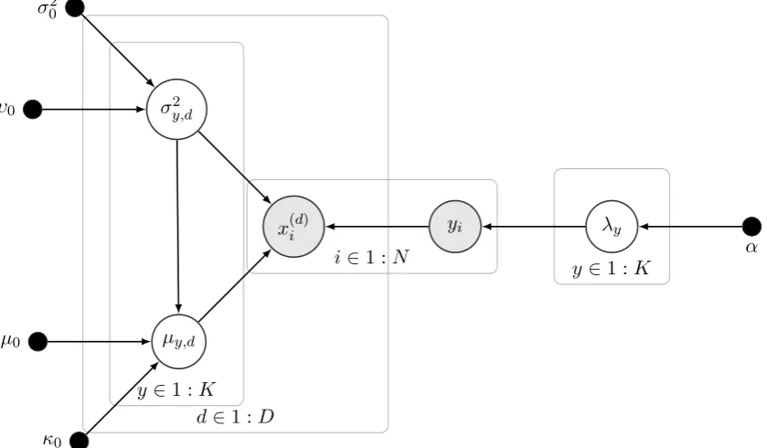
Figure 1: The probabilistic graphical model of the classifier. Shaded and white nodes are the observed and latent variables respectively; arrows represent conditional dependencies; dots represent constants (hyperparameters).

This introduces the hyperparameters,α_{={α1, ..., αK}, which can be used to encode the prior}

belief of the probability for each class. Fir this application, each class is assumed to be equally weighted, such that αy = n/K, ∀y. The dependencies of this framework are shown by the

graphical model in Figure 1, including any hyperparameters.

A small sample of labelled data, L_{, are used to establish the initial number of classes, K,} and split the measured data into groups according to their label. These data can then be used to calculate the Bayesian estimates for the model parameters. (Note, in the context of SHM, the initial measured data are regularly assumed to represent a single class, i.e. K= 1, as these measurements should, hopefully, relate to the normal-operating-condition only.) As conjugate prior distributions have been assumed, the posterior distribution over the parameter estimates can be found analytically; these are calculated for each class,y∈Y, for each dimension,d∈1 :D. Firstly, the parameters of the posterior (denoted by subscript n) are defined by [4],

κn=κ0+ny, (9a)

µn=

k0µ0+nyxy κn

, (9b)

υn=υ0+ny, (9c)

σ_n2 = 1

υn

υnσ02+

ny

X

i=1

(xy,i−xy)2+ nyκ0

κ0+ny

(µ0−xy)2 !

. (9d)

Where ny is the count (number) of observations inL with the labely, andxy is the vector of

observations labelled y. Bar notation is used to represent the sample mean. These posterior distribution for the parameters used to describe X is then defined [4],

p(µ, σ2|y,L_{)∝N Iχ}2_{(µn, κn, υn, σ}2

5

Similarly, the posterior for parameters of the categorical distribution over Y becomes [12],

p(λ_|L_)∝

K Y

y=1

λyny+αy−1_{. (11)}

In order to make class predictions on unseen data, the posterior predictive distributions for the labels,Y, and the mixture model,X, can be found analytically. This is done by marginalising out the parameters from the model. For an unlabelled measurement,xˆ_{i ={xˆ}(d)

i }Dd=1, the posterior predictive distribution is given by the student-tdistribution [4],

p(ˆx(d)|y,L) = Γ((υn+ 1)/2) Γ(υn/2)

κn

(κn+ 1)πυnσn2 1/2

1 +κn(ˆx

(d)_−µn)2

(κn+ 1)υnσn2

!−(υn+1)/2

(12)

The posterior predictive distribution overY is,

p(y|L_{) =} ny+αy

n+α0

, (13)

whereα0=PK_y=1αy [4]. By utilising the predictive posterior distributions in equations (12) and

(13), a generative classifier can be defined using Bayes rule [4], used to predict p(y|xˆ_,L_{) for the} unlabelled data inU_,

p(y|xˆ_,L_{) =} p(xˆ|y,L) p(y|L)

p(xˆ_|L₎ , (14)

which assumes independence between each dimension (feature) inX (i.e. na¨ıve Bayes), such that

p(xˆ_|y,L_{) =}

D Y

d=1

p(ˆx(d)|y,L_{). (15)}

The marginal likelihood in equation (14), which normalises the predictive distribution overY, is determined by the following integral, which is a discrete sum for a discrete random variable,

p(xˆ_|L_{) =}

Z

p(xˆ_|y,L_{) p(y|}L_{) dy≡}

K X

y=1

p(xˆ_|y,L_{) p(y|}L_{) (16)}

Note, the posterior distribution over the labels, p(y|xˆ_,L_{), is a predictive likelihood for each} class, y ∈ {1, ..., K}. That is, the likelihoods for each class are combined to give a categorical distribution, when normalised, over the label space. This is not the full posterior, which cannot be found analytically, as the student-tdistribution is not conjugate to the Dirichlet distribution. As result, the classification model is not fully Bayesian. If desired, the full posterior can be approximated via sampling algorithms (e.g. Gibbs sampling) to define a distribution over each probability estimate; however, in this work, this approach is unnecessary, as the full distribution is not required.

-4 -2 0 2 4 6

first principal component

-2 -1 0 1 2 3 4 5

second principal component

(a)

-4 -2 0 2 4 6

first principal component -2

-1 0 1 2 3 4 5

second principal component

(b)

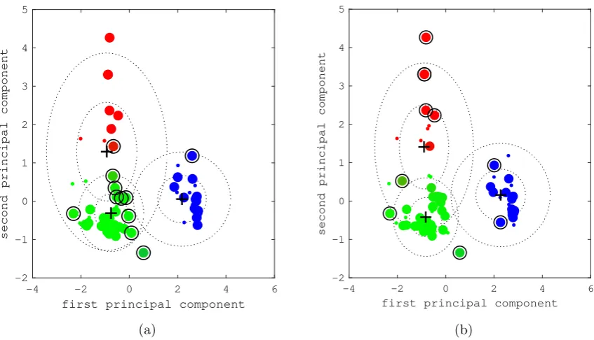
Figure 2: Data for a three-class classification problem, where the example features are extracted from acoustic emission data. Small markers are the labelled training set, L_{; large markers are the} unlabelled data,U_{, shaded according to the distribution of the label predictions p(y|}x_ˆ,L_{). The} dotted-line and + markers show the maximuma posteriori estimates of the standard deviation and cluster locations respectively. The queried data from U_{are circled; in (a) these data have} thelargest entropy; in (b) the data have the lowest maximum-likelihood.

3.1. Data query measures

In the active learning literature, there are numerous approaches to define which of the unlabelled data are the most informative [13]. Generally speaking, if labelled, these data provide the largest increase in the classification performance; however, if queries are too focussed on a specific definition of ‘informative’, the training-set built by the algorithm can be poorly representative of the underlying distribution of the data; this phenomenon is referred to as sampling bias [14]. To combat sampling bias, the query framework should not focus too much on specific regions of the feature-space; this can be achieved by combining several different definitions of ‘informative’ [15]. Usually, these measures correspond to representative or uncertain observations, according to the current estimate/model of the underlying data distribution. In this work, two probabilistic measures are utilised to direct queries.

Firstly, theentropy of the (categorical) label distribution, p(y|xˆ_,L_{), can be interpreted as a} measure of uncertainty,

H(Y) =− K X

y=1

p(y|xˆ_,L_{) logp(y|}x_ˆ,L_{). (17)}

7

start: initial training set,L

train model

p(x_{, y}|L)

new data? stop

update unlabelled set,U measured

data

predict

p(y|xˆ_,L)_,∀xˆ ∈ U

queryqb infromative

data fromU

labels provided

by the engineer update training set,L

no

yes

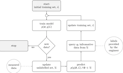
Figure 3: Flow chart to illustrate the online active learning process

Alternatively, observations inU_{with the lowest ‘maximum-likelihood’ (fromp(}x_ˆ|y,L_),∀y∈Y) can be queried. Again, querying data with a low likelihood can be seen as uncertainty sampling; however, in this case, the corresponding label distribution is not necessarily ‘mixed’. Therefore, the queried data can appear in the cluster extremities that arenot at the boundary between two or more classes; that is, the measurements are not necessarily uncertain in terms of the labels. Considering these properties, the lowest maximum-likelihood becomes suitable for querying drifting data streams, where novel data are unlikely to appear between the boundaries of existing classes.

4. An online framework

For active learning with engineering data streams in an online setting, a framework for querying data and retraining the model must be defined. There are various ways to approach this problem; for example, query by committee methods [13] can applied todrifting data streams for uncertainty sampling [10]. In this work, however, the heuristic is built around probabilistic measures from a single model. Similarly, probabilistic active learning (tree-based, i.e. nonparametric) has been applied to engineering data in previous work [7, 8]. This model also utilises uncertainty sampling, however, in this application, a large pool of the measured data are required a priori to build the tree structure, which is used for guided sampling. As a result, while the algorithm provides a significant improvement for the classification of engineering data, the heuristic applied in [7, 8] is generally unsuitable for SHM in an online setting as a large pool of data must be available to initialise the heuristic.

4.1. Guided sampling

For the experiments here, the data arrive in batches of size B, and the learner is permitted a limited number of queries per batch, qb. The initial distribution of datap(x, y|L) is learnt from

(a) (b)

Figure 4: Tool wear following inspection: (a) minor tool wear, (b) catastrophic failure of the tool.

for a large portion of the initial measured data. As a result, this model initialises as a one-class classifier [2].

The suggested active learner assumes the most informative data are defined through uncertainty sampling. Although this can risk sampling bias, as representative samples are not targeted, uncertain measurements are assumed to provide the largest increase in classification performance for this application (as is common practice in the active learning literature [13]). To address sampling bias to some extent, high entropy andleast maximum likelihood are both considered as measures of uncertainty §3.1. As discussed, this implies that uncertainty sampling occurs in the cluster extremities, as well as the boundaries between existing classes. Therefore, sampling a variety of uncertain data in this way should provided an informative training set L _from

streaming data.

As each new batch of measured data arrives, the model makes a prediction for the unlabelled data U_{, based on the labelled data seen so far}L_{. Note, the dataset}U _{includes thenew batch,} as well as unlabelled data from previous batches. The leaner then queries qb measurements

from U_{; qb/2 records are queried according to high entropy, and qb/2 are queried with the} lowest-maximum likelihood. The online process is illustrated in Figure 3. In order to assess the diagnostic performance of the learner, the dataset is split in half (using every other sample); this provides a distinct ‘moving’ test set, used to define an online performance metric (the f1-score [4] is used).

5. Experiments: machining data streams

The Element Six Ltd. (E6) machining data are an acoustic emission dataset collected from a turning machine used to manufacture metallic components. During normal operation, the cutting tool deteriorates, leading to tool wear, see Figure 4. Tool wear is undesirable, as it produces a poor surface finish for the machined component, which can lead to the onset of crack propagation, reducing the time in service for the manufactured product [16]. Consequently, it is critical to monitor tool wear, however, the machining operation must be stopped in order to inspect the tool. As a result, tool inspections are infeasible in practice, due to cost and time implications [17]. Therefore, high-value cutting tools are discarded prematurely when used in industry. For the experimental dataset used in this work, inspection of the tool is carried out using a 3D scanning microscope, the resulting images are illustrated in Figure 4.

9

of wear, acoustic emission (AE) measurements were taken during a typical machining operation, until catastrophic failure of the tool — see Figure 4b. Measurements were made by placing an AE sensor on the machine turret; these data were recorded in the time domain, and then converted into the frequency domain. Following various signal processing steps, the measured data have 129 dimensions, with 1729 observations. For further details see [17] — in this work, the measured data were collected using a similar experimental procedure, however, these tests concern the collection of data for a different machining operation.

Principal component (PCA) analysis is applieda priori to compress these data; dimension reduction is required to reduce the computation time and alleviate the curse of dimensionality. Furthermore, PCA effectively normalises the measurements, justifying the prior belief implied when building the mixture model. It should be considered that applying PCA beforehand is problematic for streaming data, as the unseen data should not be used to normalise measurements before they are available in on online setting. However, the application of PCAa priori is not considered to be major issue for the experiments presented in this work, as dimension reduction could be incorporated into the online learning process with few issues. For example, as the algorithm is applied ‘online’ bybrute force (i.e. the whole model is re-learnt for each new batch of data), the principal components can be re-extracted from the full dimensional feature space at each iteration — using the training data and bootstrap sampling.

Generally, it was found that the first 12 principal components account for 95% (1.96σ) of the total variation within these data, thus, the first 12 principal components are used to build the model, such that x_{i ∈R}12_{. As discussed, the annotation of these measurements is expensive,}

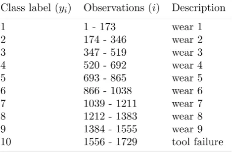
therefore, the tool was inspected at 10 regular intervals during the experiments. This corresponds to 9 different classes (ranges) of tool wear, and one class after tool failure, such thatyi∈ {1, ...,10}.

Table 1 summarises the dataset as a classification problem, and the fist 3 principal components are plotted to visualise the data in Figure 5.

Table 1: E6 Data classes

Class label (yi) Observations (i) Description

1 1 - 173 wear 1

2 174 - 346 wear 2 3 347 - 519 wear 3 4 520 - 692 wear 4 5 693 - 865 wear 5 6 866 - 1038 wear 6 7 1039 - 1211 wear 7 8 1212 - 1383 wear 8 9 1384 - 1555 wear 9 10 1556 - 1729 tool failure

By using measurements, such as the dataset presented in this work, E6 hope to accurately monitor tool wear online while keeping the number of tool investigations to annotate the measured data to a minimum. Considering this aim, the active learner is applied to the machining data as if it were online. The class labels, yi, are hidden from the algorithm, and only measurements

-15 20 -10 -5

20

pc

3

10 0

pc 2

10

pc 1

5

0

0

-10 -10

1 2 3 4 5 6 7 8 9 10

Figure 5: Scatter of the first three principal components to visualise the classification problem for the E6 data

5.1. Results

To illustrate any advantages brought about by active learning, the classifier trained using L defined by uncertainty sampling is compared to the same classifier learnt using data sampled at random from each batch. In other words, to demonstrate typical supervised learning (as a benchmark), qb data are sampled randomly fromUat each iteration, as opposed to selecting the

data with maximum entropy and the lowest maximum likelihood.

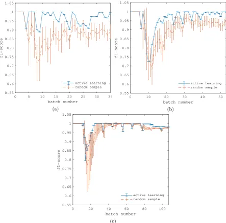
Plots are provided for a increasing label budget per iteration. The queries per batch are kept constant, such that qb = 2, while the batch size is decreased, such that B ∈ {24,16,8}. These

values correspond to query ratios of 1:12, 1:8 and 1:4, for labelled to unlabelled data respectively. For each query-budget ratio, active learning and the random sample benchmark are applied 100 times; the results are provided in Figure 6, error bars illustrate the one-sigma deviation.

5.2. Discussion

Active learning for guided sampling successfully directs queries for an increased classification performance with these data. For all query ratios, there is a clear increase in the f1-score when uncertainty sampling is used to build the training set, L_{. As to be expected, there are drops} in the classification performance as new classes are discovered by the learner; however, these are less exaggerated when an active framework is used. An additional advantage for the active learner is the consistency of the model predictions; this occurs because the data selection now follows a deterministic process. As a result, the f1-scores are consistent, because the variability associated with the ‘informativeness’ of a random sample is eliminated.

11

0 5 10 15 20 25 30 35 batch number

0.55 0.6 0.65 0.7 0.75 0.8 0.85 0.9 0.95 1 1.05

f1-score

active learning random sample

(a)

0 10 20 30 40 50

batch number 0.55

0.6 0.65 0.7 0.75 0.8 0.85 0.9 0.95 1 1.05

f1-score

active learning random sample

(b)

0 20 40 60 80 100

batch number 0.55

0.6 0.65 0.7 0.75 0.8 0.85 0.9 0.95 1 1.05

f1-score

active learning random sample

(c)

Figure 6: Online classification performance (f1-score) for various query budgets (as ratios): (a) 1:12; (b) 1:8; (c) 1:4.

5.3. Model limitations

the framework suggested in [6]; these aims are the focus of future work.

6. Conclusions

The comprehensive annotation of engineering datasets is costly/infeasible due to practical limitations; therefore, active learning techniques are suggested to define a framework for the investigation and labelling of the most informative observations when building a statistical model. This article suggests a probabilistic approach to guide queries within a sampling framework that is applied online to drifting data streams. This model is initialised as a one-class classifier (novelty detection) and adapts online as new classes are discovered — becoming a probabilistic multi-class model. In the experiments, the framework is applied to learn a model which classifies tool wear for a turning machine. Labelling these acoustic emission measurements is an expensive and time-consuming process, as it involves an engineer stopping the machining operation, and manually inspecting/scanning the cutting tool. The active learning algorithm is applied to the measured data as if they were recorded live from the machine in operation. Results show a significant increase in the diagnostic performance of the classifier when active learning is used to dictate which measured data to investigate, as opposed to the standard procedure, where the same number of observations are investigated at random; furthermore, the variability of the classification performance is significantly reduced when active learning is utilised.

Acknowledgements

The authors gratefully acknowledge the support of the UK Engineering and Physical Sciences Research Council (EPSRC) through Grant reference number EP/J016942/1. Further thanks are extended to Karen Holford and Rhys Pullin at Cardiff University for providing the AE data, and to Element Six ltd. for granting permission to use the machining data.

References

[1] Farrar C R and Worden K 2012Structural Health Monitoring: a Machine Learning Perspective (John Wiley & Sons)

[2] Moya M M, Koch M W and Hostetler L D 1993Proceedings World Congress on Neural Networkspp 359–367 [3] Schwenker F and Trentin E 2014Pattern Recognition Letters 37_{4–14 ISSN 01678655}

[4] Murphy K P 2012Machine Learning: a Probabilistic Perspective(MIT press) [5] Chapelle O, Scholkopf B and Zien A 2006Semi-Supervised Learning (MIT press)

[6] Rogers T J, Worden K, Fuentes R, Dervilis N, Tygesen U T and Cross E J 2019Mechanical Systems and Signal Processing119_{100–119 ISSN 10961216}

[7] Bull L, Manson G, Worden K and Dervilis 2019Special Topics in Structural Dynamics, Volume 5 ed Dervilis N (Springer International Publishing) pp 157–159 ISBN 978-3-319-75390-4

[8] Bull L, Worden K, Manson G and Dervilis N 2018 Journal of Sound and Vibration 437 373–388 ISSN 0022460X

[9] Wang M, Min F, Zhang Z H and Wu Y X 2017Expert Systems with Applications 85_{305–317 ISSN 09574174}

[10] Zhu X, Zhang P, Lin X and Shi Y 2007 Seventh IEEE International Conference on Data Mining (ICDM 2007)757–762 ISSN 1550-4786

[11] McCallumzy A K and Nigamy K 1998Proc. International Conference on Machine Learning (ICML)(Citeseer) pp 359–367

[12] Gelman A, Stern H S, Carlin J B, Dunson D B, Vehtari A and Rubin D B 2013Bayesian Data Analysis

(Chapman and Hall/CRC)

[13] Settles B 2012Synthesis Lectures on Artificial Intelligence and Machine Learning6_1–114

[14] Dasgupta S and Hsu D 2008Proceedings of the 25th International Conference on Machine Learning (ACM) pp 208–215

[15] Huang S J, Jin R and Zhou Z H 2010Advances in Neural Information Processing Systems pp 892–900 [16] Ghosh N, Ravi Y, Patra A, Mukhopadhyay S, Paul S, Mohanty A and Chattopadhyay A 2007Mechanical

Systems and Signal Processing21466–479