Modulations of the cosmic muon signal in ten years of Borexino data

This is a repository copy of

Modulations of the cosmic muon signal in ten years of

Borexino data

.

White Rose Research Online URL for this paper:

http://eprints.whiterose.ac.uk/136074/

Version: Published Version

Article:

Agostini, M., Altenmüller, K., Appel, S. et al. (111 more authors) (2019) Modulations of the

cosmic muon signal in ten years of Borexino data. Journal of Cosmology and Astroparticle

Physics. ISSN 1475-7516

https://doi.org/10.1088/1475-7516/2019/02/046

Reuse

This article is distributed under the terms of the Creative Commons Attribution (CC BY) licence. This licence allows you to distribute, remix, tweak, and build upon the work, even commercially, as long as you credit the authors for the original work. More information and the full terms of the licence here:

https://creativecommons.org/licenses/

Takedown

If you consider content in White Rose Research Online to be in breach of UK law, please notify us by

Journal of Cosmology and

Astroparticle Physics

OPEN ACCESS

Modulations of the cosmic muon signal in ten years of Borexino data

To cite this article: M. Agostini et al JCAP02(2019)046

JCAP02(2019)046

ournal of

C

_{osmology and}

A

_stroparticle

P

_hysics

An IOP and SISSA journal

J

Modulations of the cosmic muon

signal in ten years of Borexino data

The Borexino collaboration

M. Agostini,

K. Altenm¨

uller,

S. Appel,

V. Atroshchenko,

Z. Bagdasarian,

D. Basilico,

G. Bellini,

J. Benziger,

D. Bick,

I. Bolognino,

G. Bonfini,

D. Bravo,

B. Caccianiga,

F. Calaprice,

A. Caminata,

S. Caprioli,

M. Carlini,

P. Cavalcante,

F. Cavanna,

A. Chepurnov,

K. Choi,

L. Collica,

D. D’Angelo,

S. Davini,

A. Derbin,

X.F. Ding,

A. Di Ludovico

L. Di Noto,

I. Drachnev,

K. Fomenko,

A. Formozov,

D. Franco,

F. Gabriele,

C. Galbiati,

M. Gschwender,

C. Ghiano,

M. Giammarchi,

A. Goretti,

M. Gromov,

D. Guffanti,

C. Hagner,

T. Houdy,

E. Hungerford,

Aldo Ianni,

Andrea Ianni,

A. Jany,

D. Jeschke,

V. Kobychev,

D. Korablev,

G. Korga,

V.A. Kudryavtsev,

S. Kumaran,

T. Lachenmaier,

M. Laubenstein,

E. Litvinovich,

F. Lombardi,

P. Lombardi,

L. Ludhova,

G. Lukyanchenko,

L. Lukyanchenko,

I. Machulin,

G. Manuzio,

S. Marcocci,

J. Maricic,

J. Martyn,

S. Meighen-Berger,

E. Meroni,

M. Meyer,

L. Miramonti,

M. Misiaszek,

V. Muratova,

B. Neumair,

M. Nieslony,

L. Oberauer,

B. Opitz,

V. Orekhov,

F. Ortica,

M. Pallavicini,

L. Papp,

¨

O. Penek,

L. Pietrofaccia,

N. Pilipenko,

A. Pocar,

A. Porcelli,

G. Raikov,

G. Ranucci,

A. Razeto,

A. Re,

M. Redchuk,

A. Romani,

N. Rossi,

S. Rottenanger,

S. Sch¨

onert,

D. Semenov,

M. Skorokhvatov,

O. Smirnov,

A. Sotnikov,

L.F.F. Stokes,

Y. Suvorov,

R. Tartaglia,

JCAP02(2019)046

A. Vishneva,

R.B. Vogelaar,

F. von Feilitzsch,

S. Weinz,

M. Wojcik,

M. Wurm,

Z. Yokley,

O. Zaimidoroga,

S. Zavatarelli,

K. Zuber

and G. Zuzel

a_{Physik-Department and Excellence Cluster Universe,}

Technische Universit¨at M¨unchen, 85748 Garching, Germany

b_{National Research Centre Kurchatov Institute, 123182 Moscow, Russia}

c_{Institut f¨ur Kernphysik, Forschungszentrum J¨ulich, 52425 J¨ulich, Germany}

d_{Dipartimento di Fisica, Universit`a degli Studi and INFN, 20133 Milano, Italy}

e_{Chemical Engineering Department, Princeton University, Princeton, NJ 08544, U.S.A.}

f_{Institut f¨ur Experimentalphysik, Universit¨at Hamburg, 22761 Hamburg, Germany}

g_{INFN Laboratori Nazionali del Gran Sasso, 67010 Assergi (AQ), Italy}

h_{Physics Department, Princeton University, Princeton, NJ 08544, U.S.A.}

i_{Dipartimento di Fisica, Universit`a degli Studi and INFN, 16146 Genova, Italy}

j_{Physics Department, Virginia Polytechnic Institute and State University, Blacksburg, VA}

24061, U.S.A.

k_{Lomonosov Moscow State University Skobeltsyn Institute of Nuclear Physics,}

119234 Moscow, Russia

l_{Department of Physics and Astronomy, University of Hawaii, Honolulu, HI 96822, U.S.A.}

m_{St. Petersburg Nuclear Physics Institute NRC Kurchatov Institute,}

188350 Gatchina, Russia

n_{Gran Sasso Science Institute, 67100 L’Aquila, Italy}

o_{Joint Institute for Nuclear Research, 141980 Dubna, Russia}

p_{AstroParticule et Cosmologie, Universit´e Paris Diderot, CNRS/IN2P3, CEA/IRFU,}

Observatoire de Paris, Sorbonne Paris Cit´e, 75205 Paris Cedex 13, France

q_{Kepler Center for Astro and Particle Physics, Universit¨at T¨ubingen,}

72076 T¨ubingen, Germany

r_{Department of Physics, University of Houston, Houston, TX 77204, U.S.A.}

s_{M. Smoluchowski Institute of Physics, Jagiellonian University, 30348 Krakow, Poland}

t_{Kiev Institute for Nuclear Research, 03680 Kiev, Ukraine}

u_{Department of Physics and Astronomy, University of Sheffield,}

Sheffield S3 7RH, United Kingdom

v_{National Research Nuclear University MEPhI (Moscow Engineering Physics Institute),}

115409 Moscow, Russia

w_{RWTH Aachen University, 52062 Aachen, Germany}

x_{Institute of Physics and Excellence Cluster PRISMA,}

Johannes Gutenberg-Universit¨at Mainz, 55099 Mainz, Germany

y_{Department of Physics, Technische Universit¨at Dresden, 01062 Dresden, Germany}

1_{Present address: Universidad Aut´onoma de Madrid, Ciudad Universitaria de Cantoblanco, 28049}

Madrid, Spain.

JCAP02(2019)046

z_{Dipartimento di Chimica, Biologia e Biotecnologie,}

Universit`a degli Studi and INFN, 06123 Perugia, Italy

aa_{Amherst Center for Fundamental Interactions and Physics Department,}

University of Massachusetts, Amherst, MA 01003, U.S.A.

E-mail: spokeperson-borex@lngs.infn.it

Received August 14, 2018 Revised November 17, 2018 Accepted January 16, 2019 Published February 22, 2019

Abstract.We have measured the flux of cosmic muons in the Laboratori Nazionali del Gran Sasso at 3800 m w.e. to be (3.432_±0.003)_·10−4

m−2 s−1

based on ten years of Borexino data acquired between May 2007 and May 2017. A seasonal modulation with a period of (366.3_±0.6) d and a relative amplitude of (1.36_±0.04)% is observed. The phase is measured to be (181.7_±0.4) d, corresponding to a maximum at the 1st of July. Using data inferred from global atmospheric models, we show the muon flux to be positively correlated with the atmospheric temperature and measure the effective temperature coefficientαT= 0.90±0.02.

The origin of cosmic muons from pion and kaon decays in the atmosphere allows to interpret the effective temperature coefficient as an indirect measurement of the atmospheric kaon-to-pion production ratio r_K/π= 0.11+0−0..1107 for primary energies above 18 TeV. We find evidence for a long-term modulation of the muon flux with a period of _∼3000 d and a maximum in June 2012 that is not present in the atmospheric temperature data. A possible correlation between this modulation and the solar activity is investigated. The cosmogenic neutron production rate is found to show a seasonal modulation in phase with the cosmic muon flux but with an increased amplitude of (2.6_±0.4)%.

Keywords: neutrino detectors, neutrino experiments, cosmic rays detectors

JCAP02(2019)046

Contents

1 Introduction 1

2 The Borexino detector 2

3 Seasonal modulation of the cosmic muon flux 3

4 Atmospheric model and effective atmospheric temperature 7

5 Seasonal modulation of the effective atmospheric temperature 7

6 Correlation between muon flux and temperature 9

7 Atmospheric kaon-to-pion production ratio 10

8 Lomb-Scargle analysis of muon flux and temperature 16

9 Long-term modulation of the cosmic muon flux and the solar activity 19

10 Modulation of the cosmogenic neutron production rate 21

11 Conclusions 23

A Effective temperature weight functions 24

1 Introduction

Cosmic muons are produced mainly in the decays of kaons and pions that originate from the interaction of primary cosmic rays with nuclei in the upper atmosphere [1]. For detectors situated deep underground, the flux of cosmic muons is strongly reduced. Only muons sur-passing a certain threshold energy Ethr contribute, while lower energy muons are absorbed

JCAP02(2019)046

Borexino is an organic liquid scintillator detector situated at the LNGS, covered by a limestone overburden of 3800 m w.e. [12]. It is designed for the spectroscopy of low energy solar neutrinos that are detected via elastic scattering off electrons. Based on the data acquired after the start of data taking in May 2007, Borexino accomplished measurements of the solar 7Be [13–16],8B [17,18], pep [15,19], and pp neutrino fluxes [15,20]. The complete spectroscopy of neutrinos from the pp-chain performed with Borexino is now available in [21]. In addition, a limit on the flux of solar neutrinos produced in the CNO cycle [15, 19] and a spectroscopic measurement of antineutrinos produced in radioactive decays within the Earth, the so-called geo-neutrinos [22–24], were performed. Investigating the background to the neutrino analyses, Borexino further performed detailed studies of high energy cosmic muons as well as of cosmogenic neutrons and radioactive isotopes from muon spallation on the detector materials [25].

The Borexino detector geometry allows to identify muons passing through a spherical volume with a cross section of 146 m2_{. The detection efficiency is virtually independent of the}

muon’s incident angle, resulting in minimum systematics when measuring the muon flux and its variations. Detailed air temperature data are provided by weather forecasting centers [26] for the location of the laboratory and can be used to investigate the correlation between the flux of high energy cosmic muons and the atmospheric temperature to determine the atmospheric temperature coefficient.

In this article, we present an analysis of the cosmic muon flux as measured by Borexino based on ten years of data. In section 2, we briefly introduce the Borexino detector. In section 3, we report on the measured flux of cosmic muons and its seasonal modulation. In section 4, we introduce a model describing the expected relation between the flux of cosmic muons and the atmospheric temperature. In section 5, we present the modulation of the atmospheric temperature. In section6, we analyze the correlation between the flux of cosmic muons and the atmospheric temperature. In section 7, we use the inferred effective tem-perature coefficient to measure the kaon-to-pion production ratio in the upper atmosphere. In section 8, we further analyze both the cosmic muon flux and the effective atmospheric temperature using a Lomb-Scargle periodogram. In section 9, we report the evidence for a long-term modulation and investigate its possible correlation with the solar cycle. In sec-tion 10, we report on the seasonal modulation of the cosmogenic neutron production rate in Borexino. In section 11, we summarize our results and conclude.

2 The Borexino detector

JCAP02(2019)046

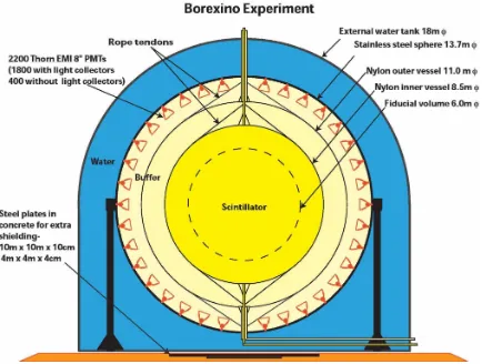
Figure 1. Schematic drawing of the Borexino detector.

the instrumentation of the outer surface of the SSS and the floor of the water tank with 208 PMTs, this Outer Detector (OD) provides an extremely efficient detection and tracking of cosmic muons via the Cherenkov light that is emitted during their passage through the water [27].

3 Seasonal modulation of the cosmic muon flux

The upper atmosphere is affected by seasonal temperature variations that alter the mean free path of the muon-producing mesons at the relevant production heights. These fluctuations are expected to be mirrored in a seasonal modulation of the underground muon flux since the high energies necessary for muons to pass through the rock overburden require that the parent mesons decay in flight without any former virtual interaction.

JCAP02(2019)046

2010 and 2011 during which the liquid scintillator target underwent further purification, no prolonged downtime of the detector is present in the data set.

Borexino features three different methods for muon identification, two of which rely on the detection of the Cherenkov light generated in the OD. The Muon Trigger Flag (MTF) is set if a trigger is issued in the OD when the detected Cherenkov light surpasses a threshold value. The Muon Clustering Flag algorithm (MCF) searches for clusters in the OD PMT hit pattern. Further, muons can be identified via their pulse shape in the ID (IDF). The mean detection efficiencies have been measured to be 0.9925(2), 0.9928(2), and 0.9890(1), respectively, and were found to remain stable. For details on the muon identification methods and the calculation of the efficiencies, we refer to [27].

In the present analysis, we define muons as events that are identified by the MCF. To account for small fluctuations of the muon identification efficiency, we estimate this efficiency for each bin and correct the measured muon rate. We discard events that do not trigger the ID to select tracks penetrating both the ID and OD volumes. Thus, the relevant detector cross section is 146 m2 as given by the radius of the SSS, independent of the incident angle of the muon. The resulting effective exposure of the data set is _∼4.2_·105_m2_{·d, in which} ∼1.2_·107 muons were detected.

Most of the muons arriving at the Borexino detector are produced in decays of kaons and pions in the upper atmosphere. In the stratosphere, temperature modulations mainly occur on the scale of seasons, while short-term weather phenomena usually only affect the tem-perature of the troposphere, with the exception of stratospheric warmings that may lead to extreme temperature increases in the polar stratosphere during winter [30]. Since the higher temperature in summer lowers the average density of the atmosphere, the probability that the muon-producing mesons decay in flight before their first virtual interaction is increased due to their longer mean free paths. Only muons produced in these decays obtain enough energy to penetrate the rock coverage and reach the Borexino detector. As a consequence, the cosmic muon flux as measured by Borexino is expected to follow the modulation of the atmospheric temperature.

At first order, the muon fluxIµ(t) may be described by a simple sinusoidal behavior as

Iµ(t) =Iµ0+δIµcos

2π

T (t−t0)

(3.1)

withI_µ0 the mean muon flux, δIµthe modulation amplitude,T the period, andt0 the phase.

Short- or long-term effects are expected to perturb the ideal seasonal modulation. Moreover, temperature and flux maxima and minima will occur at different dates in successive years.

The cosmic muon flux measured with Borexino is shown in figure 2 together with a fit according to eq. (3.1). For better visibility, the measured average muon flux per day is shown in weekly bins while the presented results are inferred applying a fit to the muon flux in a daily binning. The lower panel shows the residuals (Data₋Fit)/σ. We measure an average muon rate R0_µ = (4329.1_±1.3) d−₁

in the Borexino ID after correcting for the efficiency, which corresponds to a mean muon fluxI_µ0 = (3.432_±0.001)_·10−4

m−2 s−1

in the LNGS. The amplitude of the clearly discernible modulation isδIµ= (58.9±1.9) d−1 = (1.36±0.04)% and

we measure a periodT = (366.3_±0.6) d and a phaset0 = (174.8±3.8) d. This corresponds to

a first flux maximum on the 25th of June 2007. The statistical uncertainties of the parameters are given and the reduced χ2 _{of the fit isχ}2_{/NDF = 3921/3214. Here, we consider only the}

JCAP02(2019)046

]

-1

Average Muon Flux [d

4100 4200 4300 4400 4500

4600 _{Borexino Muon Data}

Seasonal Modulation Fit

2007 2008 2009 2010 2011 2012 2013 2014 2015 2016 2017

σ

(Data-Fit)/

6

−

4

−

2

−

0 2 4 6

Figure 2. Cosmic muon flux measured by Borexino as a function of time. The red line depicts a sinusoidal fit to the data. The lower panel shows the residuals (Data−Fit)/σ. The data are shown in weekly bins.

not accounted for in the fit function. The presence of a secondary long-term modulation that may be guessed in the residuals is investigated in sections 8 and 9.

To further analyze the phase of the seasonal modulation, we project the data to one year and fit again accordingly to eq. (3.1). The period is fixed to one year as shown in figure3. While we obtain unchanged results on the mean muon flux and the amplitude of the modulation, the phase of the strictly seasonal modulation is found to be t0= (181.7±0.4) d,

corresponding to a maximum on the 1st _{of July. We consider this as our final estimate of the}

phase of the seasonal modulation. Especially in winter and spring, clear deviations from the sinusoidal assumption of the fit may be observed that can be attributed to a more turbulent environment of the upper atmosphere due to, e.g., stratospheric warmings [30]. Thus, the reduced χ2 of the fit is χ2/NDF = 13702/362. To check the result, we selected a sample of muons as identified by the MTF and performed the same analysis steps. Consistent results were obtained and we conclude that no systematic effects based on the muon definition are introduced.

JCAP02(2019)046

Jan

Mar

May

Jul

Sep

Nov

]

-1

Average Muon Flux [d

4200 4250 4300 4350 4400 4450

10 yr Borexino Data

Seasonal Modulation Fit

Figure 3. Cosmic muon flux measured by Borexino in ten years folded to one year in a daily binning. The red line depicts a sinusoidal fit to the data with the period fixed to one year.

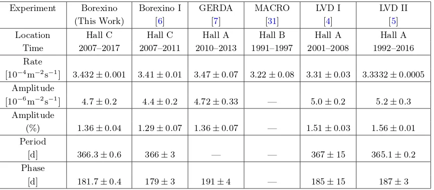
Experiment Borexino Borexino I GERDA MACRO LVD I LVD II (This Work) [6] [7] [31] [4] [5] Location Hall C Hall C Hall A Hall B Hall A Hall A

Time 2007–2017 2007–2011 2010–2013 1991–1997 2001–2008 1992–2016 Rate

[10−4_m−2_s−1_{] 3}

.432±0.001 3.41±0.01 3.47±0.07 3.22±0.08 3.31±0.03 3.3332±0.0005 Amplitude

[10−6_m−2_s−1_{] 4}

.7±0.2 4.4±0.2 4.72±0.33 — 5.0±0.2 5.2±0.3 Amplitude

(%) 1.36±0.04 1.29±0.07 1.36±0.07 — 1.51±0.03 1.56±0.01 Period

[d] 366.3±0.6 366±3 — — 367±15 365.1±0.2 Phase

[d] 181.7±0.4 179±3 191±4 — 185±15 187±3

Table 1. Results of the cosmic muon flux modulation from Borexino compared to further measure-ments carried out at the LNGS. The values of the phase of the seasonal modulation were inferred via sinusoidal fits with the period fixed to one year by all experiments.

JCAP02(2019)046

4 Atmospheric model and effective atmospheric temperature

Since the mesons, and consequently also the muons from their decays, are produced at various heights in the atmosphere, it is extremely difficult to determine the point in its temperature distribution where an individual muon was produced. In order to investigate the correlation between fluctuations of the atmospheric temperature and the cosmic muon flux observed underground, the atmosphere is modelled as an isothermal meson-producing entity with an effective temperatureTeff[2]. Teff is defined as the temperature of an isothermal

atmosphere that produces the same meson intensities as the actual atmosphere. Properly chosen weighting factors must be assigned to the corresponding depth levels accounting for the physics that determine the meson and muon production.

A common parametrization is given by [9,32]

Teff =

R∞

0 dX T(X)απ(X) +

R∞

0 dX T(X)αK(X)

R∞

0 dX απ(X) +

R∞

0 dX αK(X)

≃

PN

n=0∆XnT(Xn)(Wnπ+WnK)

PN

n=0∆Xn (Wnπ+WnK) ,

(4.1)

where the approximation considers that the temperature is measured at discrete levels Xn.

The temperature coefficients απ(X) and αK(X) relate the atmospheric temperature to the muon flux considering pion and kaon contributions, respectively. These coefficients are trans-lated into the weightsW_nπ andW_nKvia numerical integration over the atmospheric levels ∆Xn

to allow the approximation. The weights are defined in appendix A.

Figure4 shows the ten year average temperature at different pressure levels using data for the closest point to the LNGS as provided by the European Center for Medium-range Weather Forecasts (ECMWF) [26] and the assigned weights to the respective altitude levels. Higher layers of the atmosphere are assigned higher weights since muons possessing sufficient energy to penetrate the rock coverage of the LNGS are mainly produced at these altitudes. On the contrary, muons produced at lower altitudes are usually less energetic and the majority will not have the threshold energy Ethr to reach the detector.

A so-called effective temperature coefficient may be defined as

αT=

Teff I0

µ

Z ∞

0

dX W(X), (4.2)

whereW(X) =Wπ_(X)+WK_{(X). Thus, fluctuations of the cosmic muon flux may be related}

to fluctuations of the effective temperature via

∆Iµ I0

µ

=αT∆Teff Teff

(4.3)

and αT quantifies the correlation between these two observables as discussed in section 6.

5 Seasonal modulation of the effective atmospheric temperature

JCAP02(2019)046

T [K]

200 210 220 230 240 250 260 270 280 290 300

1

10

2

10

3

10

H

e

ig

h

t [

km]

10 20 30 40 50 60 Normalized Weight

0 0.1 0.2 0.3 0.4 0.5 0.6 0.7 0.8 0.9 1

Pre

ssu

re

[

h

Pa

]

Normalized Weights

Temperature Normalized Weights

!! _n$_{+ !} n

K

)

Figure 4. The ten year average temperature [26] at the location of the LNGS is shown by the red line and the normalized weighting factorsWπ

n +WnK by the black line, as functions of the pressure levels.

The right vertical axis shows the altitude corresponding to the pressure level on the left vertical axis.

data is generated by interpolating several atmospheric observables based on different types of observations (surface measurements, satellite data, or upper air sounding) and a global atmospheric model. For this analysis, we use the temperature for the location at 42.75◦

N and 13.5◦

E, which is the closest grid point to the LNGS available. The model provides atmo-spheric temperature data at 37 discrete pressure levels in the range from [0–1000] hPa four times per day at 00.00 h, 06.00 h, 12.00 h, and 18.00 h. Based on these data, we calculatedTeff

for each of the temperature sets based on eq. (4.1). The effective atmospheric temperature

Teff of the respective day was computed as the average of the four values calculated during

the day, their variance was used to estimate the uncertainty.

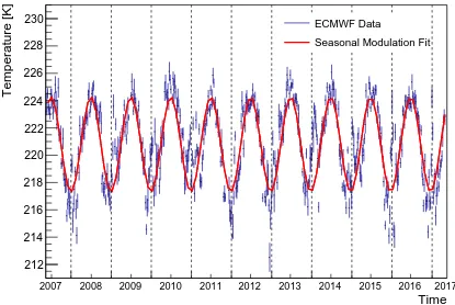
Figure5shows the mean effective atmospheric temperature in a weekly binning. Analo-gously to the cosmic muon flux, the modulation parameters were inferred by a fit to the data in a daily binning. A fit similar to eq. (3.1) returns an average effective atmospheric temperature

T_eff0 = (220.893_±0.005) K, a modulation amplitudeδTeff = (3.43±0.01) K = (1.56±0.01)%,

a period τ = (365.69_±0.04) d, and a phase t0 = (180.8±0.2) d. While period and phase

JCAP02(2019)046

Time

2007 2008 2009 2010 2011 2012 2013 2014 2015 2016 2017

Temperature [K]

212 214 216 218 220 222 224 226 228

230 _{ECMWF Data}

Seasonal Modulation Fit

Figure 5. Effective atmospheric temperature computed accordingly to eq. (4.1). The curve shows a sinusoidal fit of the data.

additional secondary maxima in winter and spring are observed. These maxima may be as-cribed to stratospheric warmings [30]. Sudden Stratospheric Warmings (SSW) sometimes even feature amplitudes comparable to the leading seasonal modulation [33], as visible e.g. in winter 2016/2017.

6 Correlation between muon flux and temperature

As expected, the modulation parameters inferred for the cosmic muon flux in section 3 and the effective atmospheric temperature in section 5 point towards a correlation of the two observables. Figure 6 shows the measured muon flux in Borexino and the effective atmospheric temperature scaled to percent deviations from their means I0

µ and Teff0 for ten

years in a daily binning. I_µ0 andT_eff0 were determined via sinusoidal fits to the respective data sets. Besides the consistency of the leading seasonal modulations of both observables, we find short-term variations of the temperature to be promptly mirrored in the underground muon flux. Exemplarily, the short-term and non-seasonal temperature increase around January 2016 generates a secondary maximum of the muon flux.

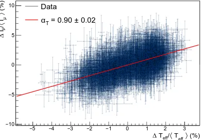
To quantify the correlation of the two observables, we plot ∆Iµ/Iµ0 versus ∆Teff/T_eff0

for each day as shown in figure 7. Indeed, we find a positive correlation coefficient (R-value) of 0.55.

JCAP02(2019)046

2007 2008 2009 2010 2011 2012 2013 2014 2015 2016 2017

Deviation from mean (%)

10

−

5

−

0 5 10 15 20 25

Borexino Muon Data

ECMWF Temperature Data

Jul/2014 Dec/2014 Jul/2015 Jan/2016

Deviation from mean (%)

10

−

8

−

6

−

4

−

2

−

0 2 4 6 8 10

Figure 6. Daily percent deviations of the cosmic muon flux and the effective atmospheric temperature from the mean in ten years of data. The insert shows a zoom for two years from May 2014 to May 2016.

In order to analyze systematic uncertainties, we performed the following checks: (1) We repeated the analysis selecting muons with our alternative muon identification method MTF. An effective temperature coefficient αT(MTF) = 0.92±0.02stat. is measured in agreement

with the above result. (2) We allowed for an offset in eq. (4.3) and fit the data. The fit provides an intercept α0 = −0.02±0.03 consistent with zero, meaning that no obvious

offsets or non-linearities are observed. (3) We performed the analysis for a two-year moving subset. We find the result to be stable and consistent with the full data set without any fluctuations above the statistical expectations. We conclude that any systematic uncertainty must be small compared to the statistical uncertainty obtained from the fit.

In table 2, the result of this analysis is compared to several further measurements performed at the LNGS. The results agree well within their uncertainties. The GERDA experiment [7] reported two values of αT using two different sets of temperature data. The

theoretical expectation ofαT at the location of the LNGS considering muon production from

both kaons and pions was formerly calculated in [6] to be 0.92_±0.02 assuming_hEthrcosθi=

1.833 TeV based on [32]. With the threshold energy_hEthrcosθi= (1.34±0.18) TeV estimated

in this paper (see section 7), the expectation isαT = 0.893±0.015. Hence, our measurement

is still in agreement with both estimations.

7 Atmospheric kaon-to-pion production ratio

JCAP02(2019)046

(%)

〉

T

〈

/

eff

T

∆

− −4 −3 −2 −1 0 1 2 3

(%)

〉

µ

I

〈

/

I

∆

10

−

5

−

0 5

10

_Data

0.02

±

= 0.90

T

α

Figure 7. ∆Iµ/Iµ0 versus ∆Teff/Teff0 with each point corresponding to one day.

Experiment Time period αT

Borexino (This work) 2007–2017 0.90±0.02 Borexino Phase I [6] 2007–2011 0.93±0.04 GERDA [7] 2010–2013 0.96±0.05 0.91±0.05 MACRO [31] 1991–1997 0.91±0.07 LVD [5] 1992–2016 0.93±0.02

Table 2. Comparison of measurements of the effective temperature coefficient at the LNGS.

depends on the production ratio of kaons and pions in the atmosphere. In the following, we infer an indirect measurement of the atmospheric kaon-to-pion production ratio based on the measurement of the effective temperature coefficient reported in section6.

For a properly weighted temperature distribution, the effective temperature coefficient

αT is theoretically predicted to be [2]

αT=

T I0

µ

∂Iµ

∂T (7.1)

with T being the temperature. The differential muon spectrum at the surface may be parametrized as [1]

dIµ

dEµ ≃

A_×E−(γ+1)

µ

1

1 + 1.1Eµcosθ/ǫπ

+ 0.38·rK/π 1 + 1.1Eµcosθ/ǫK

JCAP02(2019)046

with rK/π the atmospheric kaon-to-pion ratio, θ the zenith angle, γ = 1.78±0.05 [34] the

muon spectral index, and ǫπ = (114±3) GeV and ǫK = (851±14) GeV [9] the critical pion

and kaon energies, respectively. The critical meson energy separates the decay from the interaction regime: mesons with an energy below this energy are more likely to decay, while mesons with a higher energy most probably interact in the atmosphere before decaying.

As shown in [2], eq. (7.1) may be transformed into

αT =−

Ethr

I0 µ

∂Iµ

∂Ethr −

γ (7.3)

with the threshold energy Ethr. The muon intensity underground may be approximated for

the muon surface spectrum described by eq. (7.2) as [2,3]

Iµ≃B×E

−_γ

thr

1

γ+ (γ+ 1) 1.1_hEthrcosθi/ǫπ

+ 0.38·rK/π

γ+ (γ+ 1) 1.1_hEthrcosθi/ǫK

. (7.4)

With this approximation, the predicted αT may be calculated as

αT=

1

Dπ

1/ǫK+AK(Dπ/DK)2/ǫπ

1/ǫK+AK(Dπ/DK)/ǫπ

, (7.5)

with

Dπ,K≡ γ

γ+ 1

ǫπ,K

1.1_hEthrcosθi

+ 1 (7.6)

andAK= 0.38×rK/πdescribing the kaon contribution to the cosmic muon flux [9]. Ethrcos(θ)

is the product of the threshold energy for a muon arriving from a zenith angleθat the detector and the cosine of this angle. The mean value of this product allows to properly parametrize and compare the depths of various underground sites taking into account that the threshold energy is direction-dependent due to the shape of the respective rock overburden.

Figure 8 shows the weighted mean of αT for measurements performed at the LNGS

together with measurements at other underground laboratories from Barrett [2], IceCube [8], MINOS [9], Double Chooz [10], Daya Bay [11], and AMANDA [35]. The experimental results are plotted as a function of_hEthrcosθi, which is the parameter on whichαT explicitly

depends (eq. (7.5)–(7.6)). The insert shows the LNGS based measurements from MACRO [3], LVD [5], GERDA [7], and the two Borexino measurements from 2012 [6] and from this work. For the LNGS, a value of _hEthrcosθi = (1.34±0.18) TeV has been calculated based on a

Monte Carlo simulation (see below). The red line shows the expected αT as a function of hEthrcosθi considering muon production using the literature value of the atmospheric

kaon-to-pion ratio of r_K/π= 0.149_±0.06 [36], the dashed and dotted lines illustrate the extreme cases of pure pion or pure kaon production, respectively. The green line indicates the result of a fit to the measurements according to eq. (7.5) withr_K/πas a free parameter. We obtain

r_K/π= 0.08_±0.02stat.at a χ2/NDF = 5/9. However, note that systematic uncertainties like

the exact value of _hEthrcosθi for the respective experimental sites are not fully determined

and this result is only indicative. Also, the measured values of αT depend on the assumed

kaon-to-pion ratio since this quantity is included in the computation of Teff. We do not take

into account this inter-value dependency here.

The value of r_K/π can also be inferred indirectly from the combination of a theoretical calculation ofαT with the measurement from Borexino. In this case, no further experimental

JCAP02(2019)046

0 0.2 0.4 0.6 0.8 1 1.2 1.4 1.6 1.8 2

T

α

LNGS Weighted Mean

Ice Cube MINOS

Double Chooz ND Double Chooz FD Daya Bay EH1

Daya Bay EH2 Daya Bay EH3

Barrett AMANDA T α π ) T α ( K ) T α ( 0.02 ± = 0.08 π K/ Fit: r T α π ) T α ( K ) T α ( 0.02 ± = 0.08 π K/ Fit: r 0.85 0.9 0.95 1 Borexino Borexino LVD GERDA I GERDA II MACRO (This Work) (2012)

Figure 8. Measurements of the effective temperature coefficient αT at varying hEthrcosθi. The

curves indicate the expectedαTfor different assumptions ofrK/π, with the green curve showing a fit

of the measurements according to eq. (7.5). The insert shows the result of the present work compared to measurements from other LNGS-based experiments.

value of _hα_Ti at the location of the LNGS depending on r_K/π. For muons with an energy

Eµ≫ǫπ, which is true for the muons arriving at the LNGS, the zenith angle distribution is

best described by secθforθ <70◦

instead of the usual cos2θ[37]. We generated a toy Monte Carlo set of muons by randomly drawing a zenith angle from this distribution and an energy from the distribution given by eq. (7.2) for the respective θ. Moreover, a random azimuth angleφwas selected and the rock coverageD(θ, φ) for muons arriving from this direction was calculated based on an altitude profile of the Gran Sasso mountains obtained from the Google Maps Elevation API [38] and the density of the Gran Sasso rock ofρ= (2.71_±0.05) g/cm3[39]. We converted this into a direction dependent threshold energyEthr(θ, φ) for surface muons to

reach the LNGS using the energy loss formula given in [37] with fixed parameters. Forr_K/π

values increasing from 0 to 0.3 in steps of 0.01, we calculate the corresponding mean value of the effective temperature coefficient_hα_Ti for samples of 10000 muons with Eµ> Ethr(θ, φ).

To check our results, we performed the same calculations using the depth and zenith angle distributions of muons arriving at the LNGS predicted by the MUSUN (MUon Sim-ulations UNderground) [40] simulation code for this location. We obtain a close agreement between the two simulations with a mean difference _h∆αTi = 3.6·10−4. Additionally, we

compared the zenith angle distribution predicted by our simulation with the measured dis-tribution and found them to be in good agreement.

JCAP02(2019)046

π K/

Atmospheric Kaon to Pion Ratio r

0 0.05 0.1 0.15 0.2 0.25 0.3

T

α

0.84 0.86 0.88 0.9 0.92 0.94 0.96 0.98

T

α

Experimental

T

α

Theoretical

Fit

χ

Combined

-0.07 +0.11

= 0.11

π

K/

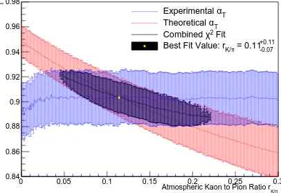
Best Fit Value: r

Figure 9. Measured value ofαT in blue and theoretical prediction in red as functions ofrK/π. The

black region indicates the 1σcontour of the intersection region ofrK/π = 0.11+0₋0..1107 around the best

fit value marked by the yellow star.

of the measurement of the muon spectral index of 0.05 [34], the uncertainties of the critical meson energies ∆ǫπ = 3 GeV and ∆ǫK = 14 GeV, and a 10% uncertainty of the drawn zenith

angle. For the combined systematic uncertainty of _hα_Ti, we found _∼ 0.015. However, the strength of several of the contributions coming from the above factors depends on rK/π. In

particular, the larger uncertainty ofǫK compared toǫπ leads to an increasing uncertainty of hα_Ti with rising r_K/π. This simulation was used as well to calculate _hEthrcosθi = (1.34±

0.18) TeV for the location of the LNGS. Also this value agrees with the result of_hEthrcosθi=

(1.30_±0.16) TeV we obtained using the MUSIC/MUSUN simulation inputs.

Figure9 shows the experimental and theoretical values ofαT as functions ofrK/π. The

experimental value of αT has a weak dependence onrK/π since it enters into the calculation

of the effective temperature Teff. To investigate this dependence, we calculated the dailyTeff

for the same range of r_K/π values as above and redetermined αT for each set ofTeff values

via the correlation to the measured muon flux as in section 6. The resulting dependence is very weak and strongly overpowered by the statistical uncertainties of the measurements. Finally, to determine the kaon-to-pion production ratio, we estimate the intersection of the two allowed αT bands to obtain a value of rK/π = 0.11−+00..1107. The allowed region in rK/π and αT has been determined by adding theχ2 profiles of the Borexino measurement and the

theoretical prediction.

JCAP02(2019)046

[GeV]

s

2

10 103

π

K/

r

0 0.05 0.1 0.15

0.2 0.25

)

atm

Borexino (this work) (p+A )

atm

MINOS (p+A )

atm

IceCube (p+A NA49 (Pb+Pb)

)

-π

/

-STAR (Au+Au, K +p) p E735 (

Figure 10. Comparison of several measurements of the kaon-to-pion production ratio. The STAR measurement was performed using Au+Au collisions at RHIC [41], the NA49 using Pb+Pb collisions at SPS [42], and the E735 using ¯p + p collisions at Tevatron [43]. The MINOS [9], IceCube [8], and Borexino measurements were performed indirectly via a measurement of the effective temperature coefficient.

JCAP02(2019)046

8 Lomb-Scargle analysis of muon flux and temperature

Besides the seasonal modulation of the cosmic muon flux underground, further physical processes might affect the cosmic muon flux and cause modulations of different periods. To investigate the presence of such non-seasonal modulations in the cosmic muon flux with Borexino, we perform a Lomb-Scargle analysis of the muon flux data.

Lomb-Scargle (LS) periodograms [45, 46] constitute a common method to identify si-nusoidal modulations in a binned data set described by

N(t) =N0·

1 +A_·sin

2πt

T +φ

, (8.1)

whereN(t) is the expected event rate at timetgiven the data set is modulated with a period

T, a relative amplitude A, and a phase φ. The LS power P for a given periodT in a data set containing ndata points may be calculated via

P(T) = 1

2σ2

Pn

j wj(N(tj)−N0) cos2Tπ(tj−τ)

2 Pn

j cos2 2Tπ(tj−τ)

+

Pn

j wj(N(tj)−N0) sin2Tπ(tj−τ)

2 Pn

j sin2 2Tπ(tj−τ)

!

, (8.2)

where N(tj)−N0 is the difference between the data value in the jth bin and the weighted

mean of the data setN0 andσ2 is the weighted variance. The weight wj=σ_j−2/hσ−_j 2i of the

jth bin is computed as the inverse square of the statistical uncertainty of the bin divided by the average inverse square of the uncertainties of the data set. The phase τ satisfies [47]

tan

4π

T ·τ

=

Pn

j wjsin(4Tπ ·tj)

Pn

j wjcos(4Tπ ·tj)

. (8.3)

Since the quadratic sums of sine and cosine are used to determine the LS power, the latter is unaffected by the phase of a modulation as long as its period is short compared to the overall measurement time.

Figure 11 shows a LS periodogram for the ten year cosmic muon data acquired with Borexino. To estimate the significance at which a peak in LS power exceeds statistical fluctuations, we use the known detector livetime distribution and mean muon rate to produce 104 white noise spectra distributed equally to the data. We define a modulation of periodT

to be significant if it surpasses a LS power Pthr that is higher than 99.5% of the values found

for white noise spectra. This threshold is indicated by the red line in figure 11.

JCAP02(2019)046

Period [d]

10 2

10 103 4

10

Lomb-Scargle Power P

3 − 10 2 − 10 1 − 10 1 10 2 10 99.5% C.L. Cosmic Muon Data

Period [d]

10 2

10 3

10 4

10

Lomb-Scargle Power P

2 − 10 1 − 10 1 10 2 10 99.5% C.L. Cosmic Muon Data

Figure 11. The left side shows the LS periodogram for the ten year cosmic muon data acquired with Borexino. Theright side shows the LS periodogram of the cosmic muon data after the seasonal modulation was subtracted statistically. The red lines indicate the significance level of 99.5%.

Period [d]

10 2

10 103 4

10

Lomb-Scargle Power P

2 − 10 1 − 10 1 10 2 10 3 10 99.5% C.L. Temperature Data Period [d] 10 2 10 3 10 4 10

Lomb-Scargle Power P

2 − 10 1 − 10 1 10 2 10 99.5% C.L. Temperature Data

Figure 12. Theleft side shows the LS periodogram for the ten year effective atmospheric temperature data at the location of the LNGS [26]. On the right side, the LS periodogram of the effective atmospheric temperature data after the seasonal modulation was subtracted statistically is shown. The red lines indicate the significance level of 99.5%.

slightly. We consider also this peak to be of physical origin and related to the minor maxima in winter and spring described in section 3, which determine a deviation from the purely sinusoidal behaviour as previously noted in [6]. Finally, a peak at the verge of significance is observed at _∼120 d.

With the period of the long-term modulation being close to our overall measurement time, the phase of the modulation is expected to affect the LS power. To investigate this, we artificially generated data samples including a seasonal and a long-term modulation of 3000 d period equally binned as the muon flux data. For each sample, the phase of the long-term modulation was altered and we computed a LS periodogram. We found the location of the peak to vary between _∼2550 d and _∼ 3750 d, which indicates the absolute uncertainty of the period. However, the long-term modulation appears as a significant peak in the LS periodogram independent of the inserted phase.

On the left panel of figure12, we show the LS periodogram of the effective atmospheric temperature. Here, only the seasonal modulation and the 180 d period are found as significant peaks. No further period surpasses the threshold power.

tem-JCAP02(2019)046

]

-1

Average Muon Flux [d

4300 4310 4320 4330 4340 4350 4360

2007 2008 2009 2010 2011 2012 2013 2014 2015 2016 2017

Borexino Muon Data

Long-Term Modulation

Figure 13. Cosmic muon flux measured by Borexino after statistically subtracting the leading order seasonal modulation in year-wide bins. The red line depicts the observed long-term modulation.

perature data. As illustrated in the right panel of figure 12, no further significant peaks are introduced by this approach. However, the 180 d period remains above the significance level, confirming our understanding of its origin. Thus, we conclude that the significant long-term modulation in the cosmic muon flux at _∼3000 d is not present in and, hence, not related to the effective atmospheric temperature.

We determine the phase and amplitude of the observed long-term modulation by fitting a function accounting for both the seasonal and the long-term modulation of the form

Iµ(t) =Iµ0+ ∆Iµ=Iµ0+δIµcos

2π

T (t−t0)

+δI_µlongcos

2π Tlong(t−t

long

0 )

(8.4)

to the daily-binned data. The fit returns a long-term modulation with a period Tlong ₌

(3010_±299) d = (8.25_±0.82) yr, a phasetlong₀ = (1993_±271) d, and an amplitudeδIµlong =

(14.7_±1.8) d−1

= (0.34_±0.04)%. Tlong is in good agreement with the period inferred from the LS periodogram and the phase of the long-term modulation indicates a maximum of the modulation in June 2012 for the investigated time frame. The parameters describing the seasonal modulation were left free in the fit and consistent results to the values reported in section3were obtained. Theχ2_{/NDF reduces from 3921/3214, when only a single modulation}

according to eq. (3.1) is fitted to the data, to 3855/3211.

JCAP02(2019)046

2007 2008 2009 2010 2011 2012 2013 2014 2015 2016 2017

Sunspot Number

0 20 40 60 80 100 120 140 160 180 200 220 240

Sunspot Data

Solar Cycle Fit

Figure 14. Daily sunspot data corresponding to the Borexino data acquisition time [51]. The curve shows a fit to the individual solar cycle.

Period [d]

10 102 ₁₀3 ₁₀4

Lomb-Scargle Power P

1

− 10

1 10

2

10

3

10 99.5% C.L.

Sunspot Data

Figure 15. LS periodogram of the daily sunspot data [51] corresponding to the time frame of the Borexino muon data acquisition. The red line indicates the significance level of 99.5%.

9 Long-term modulation of the cosmic muon flux and the solar activity

JCAP02(2019)046

An individual solar cycle can be described by a cubic power law and a Gaussian de-cline as [53]

F(t) =A

t₋ts b

3"

exp

t₋ts b

2

−c

#−₁

(9.1)

with A being the amplitude of the solar cycle, ts the starting time, b the rise time, and c an asymmetry parameter. We fit the sunspot data starting from the minimum of solar activity in March 2009 accordingly to eq. (9.1) and obtain an amplitudeA = (168.1_±0.4) sunspots per day, a start time ts= (−434±3) d prior the minimum set at the 1st of March

2009, a rise time b = (1578_±3) d, and an asymmetry parameter c= 0.000_±0.001. These parameters correspond to a maximum of the solar activity for the present cycle around the 8th of April 2013. The χ2/NDF of the fit is 143145/2672, revealing that eq. (9.1) is only a first approximation of the complex sunspot data. Note that the comparably short period indicated by the fit matches optical observations of the current solar cycle [54].

When we apply a fit similar to eq. (9.1) to the measured cosmic muon flux after sta-tistically subtracting the seasonal modulation, we obtain an amplitude A = (45.4_±8.1) muons per day, a start time ts = (−34±111) d prior the minimum set at the 1st of March

2009, a rise time b = (1208_±116) d, and an asymmetry parameter c = 1.00_±0.02 at a

χ2/NDF = 3302/2665. This indicates a maximum in March 2012.

In summary, we observe the following parameters for the long-term modulation of the cosmic muon flux and the solar sunspot activity:

Half Period/ Rise Time [d] Maximum

Muon Flux (Sinusoidal Fit) 1505_±150 16th of June 2012_± 271 d Muon Flux (Gaussian Fit) 1207_±116 4th of March 2012 _±180 d

Solar Sunspot Activity

(Gaussian Fit) 1578_±3 8th of April 2013_±5 d

The large uncertainties of the parameters of the long-term modulation of the cosmic muon flux for both fits as well as the large reducedχ2of the fit to the sunspot data indicate that the results need to be treated with care. A correlation between the solar sunspot activity and the flux of high energy cosmic muons can neither be ruled out nor clearly be proven. However, we find indications encouraging further investigation of this phenomenon, especially considering the agreement between the modulation periods observed in the LS analysis. To eventually prove or negate a correlation, longer measurement times for the underground muon flux across several solar cycles will be necessary.

Concerning the observation of a long-term muon flux modulation reported in [50], we note that: (1) the amplitude of (0.40_±0.04) % is compatible with our observation; (2) the period is also in agreement with the duration of the solar cycle; (3) the phase is however anti-correlated with the sunspot data. While the analysis of [50] includes not only MACRO and LVD but also Borexino data from [6], the latter contributes only to the last four years and seems to be in tension with the presented modulation fit.

JCAP02(2019)046

Jan Mar May Jul Sep Nov

]

-1

Neutron-producing muons [d

35.5 36 36.5 37 37.5 38 38.5

10 yr Borexino Data

Seasonal Modulation Fit

Jan Mar May Jul Sep Nov

]

-1

Neutrons [d

58 59 60 61 62 63 64

65 10 yr Borexino Data

Seasonal Modulation Fit

Figure 16. Rate of neutron-producing muons per day (left) and the cosmogenic neutron production rate (right) selecting only events with neutron multiplicityn≤10. Ten years of data are projected to a single year with monthly binning. The red line depicts a sinusoidal fit to the data with the period fixed to twelve months.

coronal magnetic field gave consistent results. However, the amplitudeδIµlong = (0.34±0.04)%

we measure for the long-term modulation of the cosmic muon flux is too high to leave a modulation of the solar shade as the sole explanation of a possible correlation.

10 Modulation of the cosmogenic neutron production rate

Cosmic muons may produce cosmogenic neutrons through various spallation processes on carbon in the Borexino organic scintillator target [56]. Neutrons are detected via the emission of a 2.2 MeV γ-ray following the capture on hydrogen or a totalγ-ray energy of 4.9 MeV after the capture on12C. The capture time isτ = (259.7_±1.3stat±2.0syst)µs [25]. As a secondary

product of cosmic muons, the number of cosmogenic neutrons is expected to also undergo a seasonal modulation. Cosmogenic neutrons have been discussed as a possible background for the expected modulation in direct searches for particle dark matter [57]. We investigate here the amplitude and phase of the cosmogenic neutron production rate.

We select cosmogenic neutrons in a special 1.6 ms acquisition gate that is opened after each ID muon [27]. Events with a visible energy corresponding to at least 800 keV are selected. The efficiency of the neutron selection has been measured to be ǫdet = (91.7±1.7stat.±

0.9syst.)% after the stabilization of the electronics baselines ∼ 30µs after the passage of a

muon. Due to the stable muon detection efficiency and no significant changes of the detector, we expect this efficiency to be stable.

We fail to observe the seasonal modulation of the cosmogenic neutron production rate, which we attribute to the occurrence of showering muons producing extremely high neutron multiplicities of up to _∼ 1000 [25] and following a non-Poissonian probability distribution. This hypothesis is sustained by the fact that an annual modulation can indeed be seen in the LS periodogram for the rate of neutron-producing muons. However, in order for the modulation to be significant in the neutron production rate, we need to remove those neutrons that are produced in high multiplicity showers from the sample.

Figure 16 shows on the left the monthly binned data of neutron-producing muons pro-jected to one year with a sinusoidal fit similar to eq. (3.1) and the period fixed to twelve months. Without efficiency correction, we obtain an average rate of neutron-producing muons R0

µn = (36.8±0.1) d −₁

, an amplitude δRµn = (0.9±0.2) d −₁

JCAP02(2019)046

Neutron Phase Amplitude Amplitude

Multiplicity Projected [months] Projected [%] Residual [%] Neutron-producing muons 6.3±0.4 2.3±0.5 2.5±0.8

n= 1 6.6±0.5 2.3±0.6 2.6±1.0 n≤2 6.1±0.3 2.6±0.5 2.8±0.8 n≤3 5.8±0.4 2.2±0.4 2.5±0.8 n≤4 6.0±0.3 2.2±0.4 2.3±0.7 n≤5 6.1±0.3 2.3±0.4 2.4±0.7 n≤10 6.0±0.3 2.6±0.4 2.7±0.7

Table 3. Parameters of the seasonal modulation observed for the number of neutron-producing muons and the neutron production rate applying increasingly high neutron multiplicity cuts. The second and third column show the phase and the amplitude of the seasonal modulation observed in the fit to the projected data, respectively. The last column shows the relative amplitude of the modulation following the residual approach.

cosmogenic neutron production rate including neutrons produced in showers featuring up to 10 neutrons shown in figure 16 on the right, we observe a rate R0_n = (61.9_±1.5) d−1

, an amplitude δRn = (1.6±0.2) d−1 = (2.6±0.4)%, and a phase t0 = (6.0±0.3) months at a χ2/NDF = 42/9. Beyond a neutron multiplicity of 10, we are unable to observe the seasonal modulation applying the LS periodogram. The observed phase is in good agreement with the seasonal modulation of the entire cosmic muon flux. However, we find the amplitude of the modulation to be higher with a difference of about 2σ compared to the relative amplitude of (1.36_±0.04)% measured for the entire cosmic muon flux in section3.

Table 3 lists the phase and amplitude of the seasonal modulation measured for the number of neutron-producing muons as well as for the neutron production rate applying increasingly high neutron multiplicity cuts. Consistent results are found for all samples with neutron multiplicities n _≤ 10 beyond which the modulation is no longer significant in the LS periodogram. We find the phase of the cosmogenic neutron production rate to agree with the muon flux. Correspondingly, the maximum occurs approximately one month later than expected for dark matter particles. However, the amplitude of the modulation is higher compared to the muon flux’s, independently of the multiplicity cut that was actually applied. To further probe this effect, we computed the average cosmogenic neutron production and neutron-producing muon rates in three summer months and three winter months for each data set. We inferred the amplitude by assuming a sinusoidal modulation around the mean of the two values. The amplitudes observed following this residual approach are listed in the last column of table 3. We find consistent values to the ones obtained from the fit in each data sample confirming the increased modulation amplitude.

The modulation of the cosmogenic neutron production rate has formerly been measured by the LVD experiment reporting an even higher modulation amplitude of δRn = (7.7±

0.8)% [58]. Since the neutron production depends on the muon energy, the larger amplitude of the modulation of the cosmogenic neutron production rate was interpreted as an indirect measurement of a seasonal modulation of the mean energy Eµ of cosmic muons observed in

JCAP02(2019)046

to verify the plausibility of this hypothesis, we have increased the mean muon energy by 1 GeV in the MUSIC/MUSUN [40] simulation codes by altering the muon spectral index (see eq. (7.2)) by 0.01. Even this small variation in the mean energy results in a 14% change in the muon flux, which is ten times larger than the amplitude of the observed annual modulation. We conclude that a modulation of the mean muon energy of several GeV is unlikely.

Additionally, we performed simulations of the muon production using the MCEq code [60] for various atmospheric models and inferred the muon surface spectra at Gran Sasso in winter and summer. We used these spectra as inputs for MUSIC/MUSUN to pre-dict the corresponding underground spectra. Based on these simulations, we obtained a difference of the cosmic muon flux between the summer and winter spectra of about 1.4% in accordance to our measurement but observed only slight deviations of the mean muon energy of less than_∼0.1 GeV.

With the exclusion of a modulation of the mean muon energy, a more complex energy dependence of the cross section for neutron production than the conventionally assumed

Eα_µ law [59] must be hypothesized to explain our observations. However, relatively large uncertainties of the atmospheric models and of the neutron production processes in the scintillator make it difficult to further investigate this percent-level effect.

11 Conclusions

We have presented a new precision measurement of the cosmic muon flux in the LNGS under a rock coverage of 3800 m w.e.using ten years of Borexino data acquired between May 2007 and May 2017. We have measured a cosmic muon flux of (3.432_±0.001)_·10−₄

m−₂ s−₁

with minimum systematics due to the spherical geometry of the detector. The seasonal modulation of the flux of high energy cosmic muons is confirmed and we have observed an amplitude of (1.36_±0.04)% and a phase of (181.7_±0.4) d corresponding to a maximum on the 1st of July. We have used data from global atmospheric models to investigate the correlation between variations of the muon flux and variations of the atmospheric temperature and showed that the seasonal modulation is also present in the effective atmospheric temperature. The correlation coefficient between the two data sets is 0.55 indicating a positive correlation and we have measured the effective temperature coefficient αT = 0.90±0.02 reducing the

statistical uncertainties of our former measurement by a factor _∼ 2. The measurement is in good agreement with theoretical estimates and previous measurements carried out at the LNGS.

We have performed a Monte Carlo simulation to calculate the theoretical expectation of αT at the location of the LNGS as a function of the atmospheric kaon-to-pion ratiorK/π.

By calculating the intersection region of the expected value and our measurement of αT in

dependence on r_K/π, we have indirectly measured r_K/π = 0.11+0−₀._.11₀₇. This measurement is compatible with former indirect and accelerator measurements and constitutes a determina-tion of rK/π in a new energy region for fixed target experiments.

JCAP02(2019)046

is required. Additionally, the physical reason for a correlation between the high energy part of the cosmic muon flux and the solar activity remains unclear.

We have analyzed the production rate of cosmogenic neutrons in the Borexino detector as well as of the number of neutron-producing muons and found a seasonal modulation in phase with the cosmic muon flux but increased amplitudes of _∼ (2.6_±0.4)% and _∼ (2.3_±0.5)%, respectively. We have shown that a strong modulation of the mean muon energy underground as an explanation of this phenomenon is disfavored by performing simulations of the muon surface spectrum in summer and winter using the MCEq software code [60] and simulating the corresponding underground spectra using the MUSIC/MUSUN codes [40].

A Effective temperature weight functions

The weights assigned to temperature measurements at different atmospheric depths Xn in

eq. (4.1) to compute the effective atmospheric temperature are defined as [9]

W_nπ(Xn)≡

A1

πe

−_Xn/Λπ(1

−Xn/Λ′π)2

γ+ (γ+ 1)B1

πK(Xn)(hEthrcosθi/ǫπ)2 ,

W_nK(Xn)≡

A1_Ke−_Xn/ΛK

(1₋Xn/Λ′K)2 γ+ (γ+ 1)B_K1K(Xn)(hEthrcosθi/ǫπ)2

(A.1)

with

K(Xn)≡

(1₋Xn/Λ′M)2

(1₋e−_Xn/Λ′ M)Λ′

M

/Xn. (A.2)

The parametersA1

K/πdescribe the relative contribution of kaons and pions, respectively, and

include the amount of inclusive meson production, the masses of mesons and muons, and the muon spectral index γ. The input parameters areA1_π = 1 andA1_K= 0.38_·r_K/π, where r_K/π

is the atmospheric kaon-to-pion production ratio. The parameter B1

K,π considers the relative

atmospheric attenuation length of the mesons, Ethr is the threshold energy a muon needs

to possess to penetrate the rock overburden and reach the LNGS, and θ is the zenith angle from which a muon is arriving. The attenuation lengths for primary cosmic rays, pions, and kaons are ΛN, Λπ, and ΛK, respectively, and 1/Λ′M≡1/ΛN−1/ΛM. ǫπ = (114±3) GeV and ǫK= (851±14) GeV are the critical meson energies separating the interaction and the decay

regimes. Since Ethr depends on the direction from which a muon arrives at the LNGS due

to the shape of the rock overburden, the median of the product of the threshold energy and the cosine of the zenith angle _hEthrcosθi is used for the computation ofTeff. Based on our

Monte Carlo simulation, _hEthrcosθi= (1.34±0.18) TeV at the location of the LNGS.

Acknowledgments

JCAP02(2019)046

References

[1] T.K. Gaisser et al.,Cosmic rays and particle physics, Cambridge University Press, Cambridge U.K. (2016).

[2] P.H. Barrett et al.,Interpretation of cosmic-ray measurements far underground,Rev. Mod. Phys.24(1952) 133[INSPIRE].

[3] MACRO_{collaboration, Seasonal variations in the underground muon intensity as seen by}

MACRO,Astropart. Phys.7(1997) 109[INSPIRE].

[4] M. Selvi,Analysis of the seasonal modulation of the cosmic muon flux in the LVD detector

during 2001-2008, in the proceedings of the 31st _{International Cosmic Ray Conference (ICRC),}

July 7–15, Lodz, Poland (2009).

[5] C. Vigorito,Underground flux of atmospheric muons and its variations with 25 years of data of

the LVD experiment, in the proceedings of the 35th _{International Cosmic Ray Conference}

(ICRC), July 12–20, Busan, South Koorea (2017).

[6] Borexino_{collaboration,Cosmic-muon flux and annual modulation in Borexino at 3800 m}

water-equivalent depth, JCAP 05(2012) 015[arXiv:1202.6403] [INSPIRE].

[7] GERDA_{collaboration,Flux modulations seen by the muon veto of the GERDA experiment,}

Astropart. Phys.84(2016) 29[arXiv:1601.06007] [INSPIRE].

[8] P. Desiati,Seasonal variations of high energy cosmic ray muons observed by the IceCube

observatory as a probe of kaon/pion ratio, in the proceedings of the 32nd _{International Cosmic}

Ray Conference (ICRC), August 11–18, Beijing, China (2011).

[9] MINOS_{collaboration,Observation of muon intensity variations by season with the MINOS far}

detector, Phys. Rev.D 81(2010) 012001[arXiv:0909.4012] [INSPIRE].

[10] Double CHOOZ_{collaboration,Cosmic-muon characterization and annual modulation}

measurement with Double CHOOZ detectors, JCAP 02(2017) 017[arXiv:1611.07845]

[INSPIRE].

[11] Daya Bay_{collaboration,Seasonal variation of the underground cosmic muon flux observed at}

Daya Bay,JCAP 01(2018) 001[arXiv:1708.01265] [INSPIRE].

[12] Borexino_{collaboration,The Borexino detector at the Laboratori Nazionali del Gran Sasso,}

Nucl. Instrum. Meth.A 600(2009) 568[arXiv:0806.2400] [INSPIRE].

[13] Borexino_{collaboration,Precision measurement of the}7_{Be solar neutrino interaction rate in}

Borexino,Phys. Rev. Lett.107(2011) 091302.

[14] Borexino_{collaboration,Absence of day-night asymmetry of862keV} 7_{Be solar neutrino rate}

in Borexino and MSW oscillation parameters,Phys. Lett.B 707(2012) 22[arXiv:1104.2150]

[INSPIRE].

[15] Borexino_{collaboration,First simultaneous precision spectroscopy of pp,}7_{Be and pepsolar}

neutrinos with Borexino phase-II, arXiv:1707.09279[INSPIRE].

[16] BOREXINO_{collaboration,Seasonal modulation of the} 7_{Be solar neutrino rate in Borexino,}

Astropart. Phys.92(2017) 21[arXiv:1701.07970] [INSPIRE].

[17] Borexino_{collaboration,Measurement of the solar} 8_{B neutrino rate with a liquid scintillator}

target and3 MeV energy threshold in the Borexino detector,Phys. Rev.D 82(2010) 033006

[arXiv:0808.2868] [INSPIRE].

[18] Borexino_{collaboration,Improved measurement of} 8_{B solar neutrinos with 1.5 kt y of}

Borexino exposure, arXiv:1709.00756[INSPIRE].

[19] Borexino_{collaboration,First evidence of pep solar neutrinos by direct detection in Borexino,}

JCAP02(2019)046

[20] BOREXINO_{collaboration,Neutrinos from the primary proton–proton fusion process in the}

Sun,Nature 512(2014) 383[INSPIRE].

[21] Borexino_{collaboration,Comprehensive measurement ofpp-chain solar neutrinos,Nature 562}

(2018) 505.

[22] Borexino_{collaboration,Observation of geo-neutrinos,Phys. Lett.}B 687(2010) 299

[arXiv:1003.0284] [INSPIRE].

[23] Borexino_{collaboration,Measurement of geo-neutrinos from 1353 days of Borexino,Phys.}

Lett.B 722(2013) 295[arXiv:1303.2571] [INSPIRE].

[24] Borexino_{collaboration,Spectroscopy of geoneutrinos from 2056 days of Borexino data, Phys.}

Rev. D 92(2015) 031101[arXiv:1506.04610] [INSPIRE].

[25] Borexino_{collaboration,Cosmogenic backgrounds in Borexino at3800m water-equivalent}

depth,JCAP 08(2013) 049[arXiv:1304.7381] [INSPIRE].

[26] D.P. Dee et al.,The ERA-Interim reanalysis: configuration and performance of the data

assimilation system, John Wiley & Sons Ltd., U.S.A. (2011).

[27] Borexino_{collaboration,Muon and cosmogenic neutron detection in Borexino,2011JINST} 6

P05005[arXiv:1101.3101].

[28] E. Gschwendtner et al.,Performance and operational experience of the CNGS facility, in proceedings of the 1st _{International Particle Accelerator Conference (IPAC’11), May 23–28,}

Kyoto, Japan (2010).

[29] Borexino_{collaboration,Measurement of CNGS muon neutrino speed with Borexino,Phys.}

Lett.B 716(2012) 401[arXiv:1207.6860] [INSPIRE].

[30] D.G. Andrews et al.,Middle atmosphere dynamics, Academic Press, New York, U.S.A. (1987).

[31] MACRO_{collaboration, The search for the sidereal and solar diurnal modulations in the total}

MACRO muon data set,Phys. Rev.D 67(2003) 042002[astro-ph/0211119] [INSPIRE].

[32] E.W. Grashorn et al.,The atmospheric charged kaon/pion ratio using seasonal variation

methods, Astropart. Phys.33(2010) 140[arXiv:0909.5382] [INSPIRE].

[33] MINOS collaboration,Sudden stratospheric warmings seen in MINOS deep underground muon

data,Geophys. Res. Lett.36(2009) L05809.

[34] LVD_{collaboration,Muon ‘Depth intensity’ relation measured by LVD underground experiment}

and cosmic ray muon spectrum at sea level,Phys. Rev.D 58(1998) 092005 [hep-ex/9806001]

[INSPIRE].

[35] A. Bouchta,Seasonal variation of the muon flux seen by AMANDA, in the proceedings of the

27th _{International Cosmic Ray Conference (ICRC), August 8–15, Hamburg, Germany (2001).}

[36] G.D. Barr, T.K. Gaisser, S. Robbins and T. Stanev,Uncertainties in atmospheric neutrino

fluxes,Phys. Rev.D 74 (2006) 094009[astro-ph/0611266] [INSPIRE].

[37] Particle Data Group_{collaboration,Review of particle physics,Chin. Phys.C 40(2016)}

100001[INSPIRE].

[38] Google Maps Elevation API,

https://developers.google.com/maps/documentation/elevation/intro.

[39] MACRO_{collaboration, Vertical muon intensity measured with MACRO at the Gran Sasso}

Laboratory, Phys. Rev.D 52(1995) 3793[INSPIRE].

[40] V.A. Kudryavtsev,Muon simulation codes MUSIC and MUSUN for underground physics,

Comput. Phys. Commun.180(2009) 339[arXiv:0810.4635] [INSPIRE].

[41] STAR_{collaboration,Kaon production and kaon to pion ratio in Au+Au collisions at}

√_s