Abstract—Vehicle emissions variations impose significant challenges to the automotive industry. In these simulation studies, nonlinear estimation techniques based on state-dependent and extended Kalman filtering are developed for spark ignition engines to enhance robustness of the feedforward fuel controllers to changes in nominal system parameters and measurement errors. A model-based approach is used to derive the optimal filters. Numerical simulations indicate the superiority of estimation-based approaches to enhance robustness of in-cylinder air estimation which directly contributes to the precision of engine exhaust air-fuel ratio and, consequently the consistency of the tailpipe emissions. The results obtained are for an aggressive driving profile and are presented and discussed.
I. INTRODUCTION
There are inherent limitations in the accuracy of sensors, actuators and various components for real-time engine control. The sources of these variations are either in the manufacturing processes or through the normal degradation over the life of components. While tighter manufacturing tolerances can reduce these variations, the actual cost may be prohibitive. An alternative approach is to design controllers with a built-in capability for more robust performance in the presence of reasonable variations in the component characteristics and the process uncertainties. At the same time, in the absence of information about the nature of variations and their characteristics for sensors and actuators, and engine processes, the design may lead to over specification and unnecessary cost escalation. One solution is to develop a mathematical model of the process, including sensors and actuators, and through simulation analysis determine the salient components contributing the most to the quantity of interest. The impact of each component variation, in isolation and in combination with other components, can be simulated numerically and evaluated. Model-based filter designs to compensate for the process and measurement errors and to obtain the best estimates for the quantities of interest will first develop. This will use nonlinear estimation techniques, such as the state-dependent Kalman filtering and extended Kalman filtering methods
Manuscript received September 10, 2005
A. Dutka is with ISC Ltd., Glasgow, UK ([email protected]),
H. Javaherian is with GM R&D, Warren, MI, USA, ([email protected])
M. J. Grimble is with the University of Strathclyde, Glasgow, UK ([email protected])
In this application, we are concerned with important engine variables such as the throttle position, the intake manifold pressure and temperature. Clearly, all these intake manifold variables contribute directly to the cylinder air charge. Due to significant time-delays between the process actuation and the measurements, that is inherent in the engine processes, a closed loop control is always too slow and as a result the control performance will suffer [1]. The remedy is to focus on the design of a responsive feedforward controller. The engine air-fuel ratio is one of the most significant variables of interest with the most impact on tailpipe emissions. We will focus our attention on the design of a robust feedforward controller for fuel control system. This requires a “predictive” control capability in the estimation of the cylinder air charge before the required amount of fuel is calculated and injected. The resulting models will be the basis for various filter designs and the subsequent analysis of the systems response to component analysis.
It is clear that the systems structure imposes performance constraints due to the system model uncertainties that may be modeled using random process noise and by the sensor uncertainty that may be modeled by the noise. In practice this determines the upper bound for control system performance that will not be achieved in reality. The model-based filtering methods are capable of both reconstructing the state of the system and filtering the noise from the measurements. The feedforward controller relies upon these measurements and any improvement in the accuracy will result in an improvement of the precision of the air-fuel ratio control.
A mathematical evaluation of the resulting nonlinear dynamic system is difficult to achieve, but Monte-Carlo simulation tools may be used to assess the envelope of variations for a wide range of process variations that are due to components and measurements errors.
II. THE INTAKE MANIFOLD MODEL
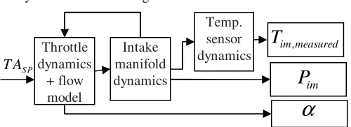
[image:1.612.313.563.612.703.2]The block diagram of the intake manifold and the throttle subsystem is shown in Fig. 1.
Fig. 1: System diagram
State-Dependent Kalman Filters for Robust Engine Control
Arkadiusz Dutka, Hossein Javaherian and Michael J. Grimble
im
P
SP T A
Throttle dynamics
+ flow model
Intake manifold dynamics
Temp. sensor
dynamics im measured,
T
α
Proceedings of the 2006 American Control Conference
The electronic throttle is powered by an electric motor and is controlled locally by its dedicated controller. The drive-by-wire actuator with its controller may be modeled by a second order continuous time linear system [1].
The system is described by the event-based discrete time model, Ts n, =120 8
(
Nn)
[ ]
s , where Nn is the engine speedin revolutions per minute at the discrete event n.
The discretized electronic throttle model is described by the equation (1) to follow. A non-minimal representation of the original 2nd order system with 3 states was used due to better numerical properties for systems discretized with variable sampling rate. The process noise that introduces a stochastic system uncertainty is also included in the model.
, 1 , , , , ,
, ,
ET n ET n ET n ET n SP n ET n
n ET ET n ET n
x A x B TA w
TA C x v
+ = + +
= + (1)
In equation (1) TAn denotes the measured throttle angle.
The throttle position sensor dynamics are very fast and may be neglected. TASP n, is the throttle angle command
(setpoint), wET n, is the throttle actuator process noise, vET n,
is the throttle position measurement noise and the system:
[
]
(
)
(
)
(
)
(
)
, 2, 1, 2, , 1,
1, , , 0 ,
2
2, , , 0 , ,
2 2
1, , , 2, ,
2
, 0 , 0
,
0 0 0 1
; ;
0 1 0 0
0 1 0 ; 1 ;
;
2 ;
exp ; 1 ;
cos
ET n n n n ET n n
ET n ET n ET n ET n ET
n ET n ET n ET n ET ET n
n ET n ET n n ET n
ET n s n ET
ET n
A b a a B b
C b
b
a a
T
α β ζω γ ω
α α ζω γ ω β
α β α
α ζω ω ω ζ
β ω
⎡ ⎤ ⎡ ⎤
⎢ ⎥ ⎢ ⎥
=⎢ ⎥ =⎢ ⎥
⎢ ⎥ ⎢ ⎥
⎣ ⎦ ⎣ ⎦
= = − +
= + −
= − =
= − = −
=
(
ETTs n,)
;γET n, =sin(
ωETTs n,)
.0, throttle parameters
ω ζ −
It should be noted that due to the variable sampling rate
,
s n
T the model must be re-discretized at each discrete event.
Alternatively, if the computational burden associated with the discretization is too heavy an approximate Euler integration method may be employed or discrete time model could be stored in a lookup table.
The equations (2), (3) give the expression for nonchoked/choked flow through the throttle [2], [3]. The throttle position is given by α =n C xET ET n, . For nonchoked
flow the following model is used:
1 1
, ,
,
, ,
1 ,
, 2
1 1
2 , 1
im n im n
at n n
a n a n
im n
a n
P P
m
P P
P if
P
κ
κ κ
κ κ κ κ
κ
−
−
⎡ ⎤
⎛ ⎞ ⎢ ⎛ ⎞ ⎥
= Ξ ⋅⎜⎜ ⎟⎟ ⎢ −⎜⎜ ⎟⎟ ⎥ −
⎝ ⎠ ⎢⎣ ⎝ ⎠ ⎥⎦
⎛ ⎞
>⎜⎝ + ⎟⎠
(2)
For choked flow the model is given by the equation:
( 1)
2 1 ,
1 ,
, 2
1 2
1
at n n
im n
a n
m
P if
P
κ κ
κ κ κ
κ
κ + ⋅ −
−
⎛ ⎞
= Ξ ⋅ ⎜ ⎟ −
⎝ ⎠
⎛ ⎞
≤⎜⎝ + ⎟⎠
(3)
where Ξ =n Cd n, ⋅Ath
( )
αn ⋅Pa n, Rair⋅Ta n, , mat n, is thethrottle mass flow rate, Cd n, =Cd n,
(
Pim n, Pa n, ,αn)
is thedischarge coefficient modeled by the lookup table, Ath
( )
αnis the throttle cross-sectional area, Pa n, is the upstream pressure (ambient), Ta n, is the upstream temperature (ambient), Pim n, is the downstream pressure (intake manifold), κ is the ratio of specific heats for dry air, Rair is the ideal gas constant for dry air.
The cross-sectional area Ath
( )
αn is a function of thethrottle body dimensions and the angle between the closed and current throttle position. In a very simplified form it may be given by the following equation:
( )
2(
( )
)
1 cos
th n th n
A α = ⋅π R − α (4)
where: Rth- radius of the throttle.
The non-linear intake manifold dynamics are discretized with the Euler method. The deterministic two state non-linear discrete time model of the intake manifold is given by the following equations:
,
, 1 , , , ,
1
1 air a n
im n cyl n im n s n at n s n ext
im im im
R T
P V P T m T Q
V V V
κ
κ η κ
+
⎛ ⎞ −
= −⎜ ⎟ + +
⎝ ⎠
(5)
, ,
2 ,
, , , , , , ,
, , ,
1
1 1
1
im n cyl n im n
im
air a n air
im n im n s n at n im n s n ext n
im im n im im n im im n
T V T
V
R T R
T T T m T T Q
V P V P V P
κ η κ
κ κ
⎛ ⎛ ⎞⎞
= −⎜ ⎜⎝ − ⎟⎠⎟ +
⎝ ⎠
⎛ − ⎞ + −
⎜ ⎟
⎜ ⎟
⎝ ⎠
(6)
where Qext =h T1
(
coolant−Tim)
+h T2(
a−Tim)
- heat transferequation, h1 - heat transfer coefficient (from the engine), h2
- heat transfer coefficient (from ambient temperature), Pim
is the intake manifold pressure [kPa], Tim is the intake
manifold temperature [K], Ta is the ambient temperature
[K], Tcoolant is the engine coolant temperature [K], Vim is the
intake manifold volume [ 3
dm
⎡ ⎤
⎣ ⎦],Vd is the engine displacement [dm3
], η η=
(
N P, im)
is the volumetricefficiency [-] and N is the engine speed [rpm].
, 1 , , , ,
, , , im, ,
IM n IM n IM n IM n n EM n
im meas n IM IM n P n EM n
x A x B TA w
P C x f v
+ = + ⋅ +
= + + (7)
The stochastic process noise wEM n, is introduced in this model. The pressure sensor has negligible (fast) dynamics and may be modeled by the static output equation with the measurement noise vEM n, . The state dependent matrices of the model (7) are of the following form:
, , , , , , , , . , , , , , , 1 1 1 1
0 1 1
( ) 1 im n IM n im n cyl
n s n ext
im im n im
IM n
cyl
n s n ext
im im im
air a n s n at n
im ET ET n
IM n
air a n
im n im
im im n
P x
T
V
T Q
V T V
A
V
T Q
V V P k
R T T m
V C x
B
R T
T T
V P
κ η κ
κ η κ
κ κ κ ⎡ ⎤ =⎢ ⎥ ⎣ ⎦ ⎡⎛ ⎞ − ⎤ − ⎢⎜ ⎟ ⎥ ⎝ ⎠ ⎢ ⎥ =⎢ ⎥ ⎛ ⎛ ⎞⎞ − ⎢ ⎜ − ⎜ − ⎟⎟+ ⎥ ⎢ ⎝ ⎝ ⎠⎠ ⎥ ⎣ ⎦ ⎛ ⎞ ⎜ ⎟ ⎝ ⎠ = −
[
]
2 , , , , ,; 1 0
1 IM
air
n s n at n im im n ET ET n
C R
T m
V P C x
⎡ ⎤ ⎢ ⎥ ⎢ ⎥ = ⎢⎛ ⎞ ⎥ ⎢⎜ ⎟ ⎥ ⎜ ⎟ ⎢⎝ ⎠ ⎥ ⎣ ⎦
The port flow rate is modeled as a function of the intake gas density, engine displacement and volumetric efficiency:
, ,
,
120
im n n d ac n
air im n
P N V
m
R T
η =
(8)
The intake manifold air temperature is measured by a relatively slow sensor. The discrete-time model of this sensor is given by the equation (9).
. , 1 . , , . ,
. , . , . ,
im meas n T im meas n T IM n im meas n
im out n im meas n im meas n
T a T b x w
T T v
+ = + +
= + (9)
The wim meas n, , is the temperature sensor process noise,
, ,
im meas n
v is the temperature measurement noise and model
parameters are as follows:aT =exp
(
−Ts τTemp)
;(
)
0 1 exp
T s Temp
b =⎡⎣ − −T τ ⎤⎦. The τTemp is a time constant
of the sensor.
The final augmented model is given by the following set of equations:
1
n n n n n n
n n n n
x A x B u w y C x v
+ = + +
= + (10)
where
, ,
, , ,
. , . , . ,
; ; ;
ET n n ET n
n IM n n im n n IM n
im meas n im out n im meas n
x TA w
x x y P w w
T T w
⎡ ⎤ ⎡ ⎤ ⎡ ⎤ ⎢ ⎥ ⎢ ⎥ ⎢ ⎥ =⎢ ⎥ ⎢= ⎥ =⎢ ⎥ ⎢ ⎥ ⎢ ⎥ ⎢ ⎥ ⎣ ⎦ ⎣ ⎦ ⎣ ⎦ , , , , . , 0 0
; 0 ;
0
ET n ET n
n IM n n IM n ET IM
im meas n T T
v A
v v A B C A
v b a
⎡ ⎤ ⎡ ⎤
⎢ ⎥ ⎢ ⎥
=⎢ ⎥ =⎢ ⎥
⎢ ⎥ ⎢⎣ ⎥⎦
⎣ ⎦
, 0 0
0 ; 0 0 .
0 0 0 1
ET n ET
n n IM
B C
B C C
⎡ ⎤ ⎡ ⎤ ⎢ ⎥ ⎢ ⎥ =⎢ ⎥ =⎢ ⎥ ⎢ ⎥ ⎢ ⎥ ⎣ ⎦ ⎣ ⎦ n
w
andv
n are independent white Gaussian noise signals with cov{ }
wn =Q and cov{ }
vn =R. The Q and Rare diagonal semi-positive and positive definite matrices, respectively.
III. STATE DEPENDENT KALMAN FILTER
In the paper the discrete time Kalman filter for nonlinear systems is considered. The results obtained from the SDKF will be related to the standard recursive Extended Kalman Filter formulation [5]. Consider the model of the system is given by the following discrete time state-space equations:
1
n n n n n n
n n n n
x A x B u w
y C x v
+ = + +
= + (11)
where xn is n×1 state vector, un is p×1 control vector,
n
y is q×1 output vector. The matrices An =A x
( )
n ,( )
n n
B =B x , Cn =C x
( )
n are functions of state.Additionally it is assumed that
{
,}
n x
n n
x∀∈Ω C A is point-wise observable [3] in the operating region Ωx. The process
noise wn and measurement noise vn are independent white
Gaussian signals with cov
{ }
wn =Q and cov{ }
vn =R. Qand R are diagonal semi-positive and positive definite matrices, respectively.
In this work, a modified Kalman filter based on the state-dependent representation is used. The state-state-dependent Kalman filter was introduced by Mracek [6]. This was an extension of the state-dependent Riccati equation control method. The discrete version of the state-dependent Kalman filter is given by the following equations:
(
)
(
)
1 ˆ ˆ ˆ
ˆ ˆ ˆ
ˆ ˆ ˆ
n n n n n n n n n
n n n
x A x K y C x B u
y C x
+ = ⋅ + − +
= (12)
The state dependent model matrices are denoted as
( )
( )
( )
ˆ ˆ ,ˆ ˆ , ˆ ˆ
n n n n n n
A =A x B =B x C =C x . The filter gain Kn is
given by the following equation:
(
)
1ˆT ˆ ˆT
n n n n n n n
K =P C C P C +R − (13)
The
P
n is the solution of the discrete algebraic Riccati equation(
)
1ˆ ˆT ˆ ˆT ˆ ˆT
n n n n n n n n n n n
P =A ⎢⎡P −P C R C P C+ − C P⎤⎥A +Q
⎣ ⎦
(14)
( )
( )
( )
ˆ ˆ , ˆ ˆ ,ˆ ˆ
n n n n n n
A =A x B =B x C =C x are based on the state
estimates. An estimation bias may result in model mismatch. This may cause the state estimates to diverge. The convergence analysis of the filter, for a general non-linear system representation, is not possible. The properties of the filter must be analyzed for the particular application. The type of non-linearity is an important feature for the analysis. In practice a pseudo convergence analysis may be carried out through simulation tests.
IV. THE STOCHASTIC NOISE FILTERING SETUP
The filtering and estimation simulation experiments use the model presented in previous section. Unmodeled engine parameters logged in the US06 driving cycle dataset (i.e. the engine speed, ambient conditions, the throttle position setpoint) are used in the simulation as external parameters. The engine model and the data are of a sport vehicle with 5.7 L V8 engine driven on US06 driving cycle on a chassis roll. For the data collection purpose the engine was controlled by a non-production rapid prototyping setup.
The air-fuel ratio control system performance strongly relies on the precision of the cylinder air charge (CAC) prediction. The CAC prediction precision relies on the accuracy of the engine parameter measurements. Noise and deterministic biases deteriorate the model-based CAC prediction. The accuracy assessment is effected by comparing the simulated delayed engine CAC with the feedforward controller internal prediction [7]. Stochastic process and measurement noise is injected into the model. Since the air-fuel ratio control accuracy is proportionally influenced by the accuracy of the future CAC estimation, the CAC prediction mismatch computed as
(
)
100% CACpred CACactual CACactual
ε = ⋅ − is a good metric
for the control system performance.
Process noise introduced in the system has the following covariance Q:
{ }
(
{
,} {
,} {
. ,}
)
cov n cov ET n , cov IM n , cov im meas n
Q= w =diag w w w
{
,}
(
)
cov wET n =diag 0, 1.95 -6, 0e
{
,}
(
)
{
. ,}
[ ]
cov wIM n =diag 2.5 -3, 1 -2 , cove e wim meas n = 1 -4e
The measurement noise is characterized by the covariance matrix
R
:{ }
(
{ } { }
, ,{
. ,}
)
cov n cov ET n , cov IM n , cov im meas n
R= v =diag v v v
{ }
,{ }
,cov vET n =7.62 -5, cove vIM n = −1e 2
{
. ,}
cov vim meas n =2.5e−3
The extended and state-dependent Kalman filters (EKF and SDKF) were used for the reconstruction of the state when there are noisy measurements. The simulation
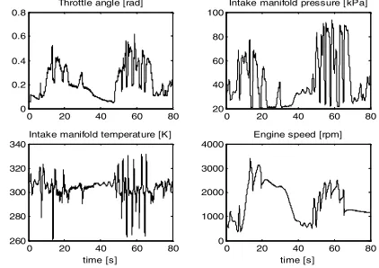
involves the throttle actuator, the throttle flow and the intake manifold two-state models. The cylinder air charge (CAC) is used within the feedforward (FF) controller. The accuracy of the CAC prediction is used as a benchmark of the control performance. The FF controller inputs are either direct measurements of intake manifold pressure, indicated throttle position and intake manifold temperature or estimates of these variables obtained from the EKF or SDKF. Also, for fair comparison, a test where the intake manifold temperature is supplied by an open-loop observer is carried out. The SDKF results are compared with the direct measurements approach results. The simulation tests are carried out with the engine parameters taken from the driving cycle data shown in Fig. 2. The controller inputs that are either estimates or direct measurements are compared with the actual intake manifold and throttle states.
0 20 40 60 80
0 0.2 0.4 0.6 0.8
Throttle angle [rad]
0 20 40 60 80
20 40 60 80 100
Intake manifold pressure [kPa]
0 20 40 60 80
260 280 300 320 340
Intake manifold temperature [K]
time [s]
0 20 40 60 80
0 1000 2000 3000 4000
Engine speed [rpm]
[image:4.612.329.540.275.424.2]time [s]
Fig. 2: Engine simulation parameters
The indicator of ‘method efficiency’ used in this analysis is the cylinder air charge prediction. As described, the feedforward (FF) controller used in the simulation employs a throttle actuator model for future throttle trajectory prediction. This trajectory prediction is used by FF controller to generate the cylinder air charge (CAC) prediction. The 6-event prediction is compared with the actual cylinder air charge being an internal variable of the simulated intake manifold. The accuracy of the CAC prediction over the simulation time of 80 seconds is evaluated based on the integrated absolute and squared error value. The results of the simulations are presented and analyzed below. The error signal measures are presented in Table 1.
Simulation setup Direct measure.
Direct measure.+OL
estimation
SDKF EKF
actual predicted
CAC −CAC
∑
15376 9943 7124 7101(
)
2actual predicted
CAC −CAC
∑ 61437 25435 15913 15817
The results indicate that the extended Kalman filter provides the best accuracy. The state-dependent Kalman filter, however, gives very similar results. Note that the Kalman gains used for the SDKF result from the solution of the algebraic Riccati equation. This provides suboptimal steady state solution. However, it is easier to simplify such filter for an implementation purpose by means of lookup tables. Results obtained using the estimation methods when compared to direct measurement methods indicate that improved cylinder air charge prediction is achievable. This improved CAC prediction, of course, directly results in significantly improved air-fuel ratio control precision.
V. THE PARAMETER VARIATION FILTERING SETUP
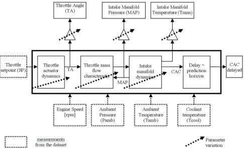
[image:5.612.311.557.146.383.2]The results presented in the previous section indicate improved cylinder air charge (CAC) prediction accuracy when either extended or state-dependent Kalman filters (EKF, SDKF) are used. The derivation of the EKF (or SDKF) is based on the assumption that the process and measurement noise signals are stochastic. This method of modeling – especially for the model mismatch represented by the process noise is not always accurate. In this section a deterministic parameter variation is introduced in the intake manifold and throttle model. Additionally, sensor gain errors are introduced for throttle position, intake manifold pressure and temperature measurements. The system diagram including an indication of the point of introduction of the parameter variation/uncertainty is shown in Fig. 3.
Fig. 3: Engine simulation block – parameter variation
A Monte-Carlo parameter variation analysis was conducted next. The parameters that were determined to be subject to variation are displayed in Table 2. A truncated Gaussian probability distribution is assumed within the parameter variation limits.
The results of the simulations are presented and analyzed now. The analysis of results reveals that the SDKF and EKF filters improve the robustness of the cylinder air charge estimation to the combination of modeling and measurement errors proposed in Table 2.
Better performance is indicated in any given histogram ( Fig. 4, Fig. 5) by a higher number of simulation results (with either absolute or squared integrated error values) occurring at the lower error levels. In each container in the histogram the number of simulation results with the integrated squared or absolute error within the limits is counted.
Parameter of interest Parameter variation limits
modelled actual actual
100
par
par par
par
ε = ⎛⎜ − ⎞⎟
⎝ ⎠
T
ζ
in (1)5 %
[ ]
T
ζ
ε
= ±
T
ω
in (1)5 %
[ ]
T
ζ
ω
= ±
d th
C
⋅
A
in (2), (3)3 %
[ ]
d th
C A
ε
⋅= ±
1
h
in (5), (6)[ ]
1
5 %
h
ε
= ±
2
h
in (5), (6)[ ]
2
5 %
h
ε
= ±
(
N P
,
im)
η η
=
in (5),(6)ε
η= ±
4 %
[ ]
,
im meas
T
measurement error[ ]
,
2 %
im meas
T
ε
= ±
im
P
measurement error2 %
[ ]
im
P
ε
= ±
α
measurement error3 %
[ ]
α
[image:5.612.56.299.424.577.2]ε
= ±
Table 2: Assumed parameter, measurement error variations
Obviously the best possible case would have all results within the lowest error limits. The accuracy of the statistical method used here relies on a large number of simulations being carried out. Histograms for the CAC prediction error indicate significant improvement over open-loop observer. The mean error values computed based on all of 2000 simulations also indicate superiority of the EKF/SDKF methods over the conventional methods based on direct measurements
0 1 2 3 4 5 6 7 8 9
x 104
0 200 400 600 800 1000 1200 1400 1600
CAC integrated squared error
error level
R
e
su
lt
s co
u
n
t
Pressure, Thr. angle measured, OL temperature Pressure, Temperature and Thr. angle measured SDKF
EKF
0 2000 4000 6000 8000 10000 12000 14000 0
100 200 300 400 500 600 700 800 900
CAC integrated absolute error
error level
R
e
su
lt
s co
u
n
t
Pressure, Thr. angle measured, OL temperature Pressure, Temperature and Thr. angle measured SDKF
[image:6.612.65.285.55.231.2]EKF
Fig. 5: CAC int. absolute error histogram
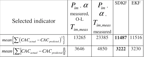
The results are gathered in Table 3. The SDKF provides the best overall results in this comparison. This indicates that in the presence of model mismatch, this filtering method is likely to provide the best robust performance among the techniques considered.
Selected indicator
im
P
,α
measured,O-L
,
im meas
T
im
P
,α
,,
im meas
T
measured
SDKF EKF
( )
{
2}
actual predicted
mean ∑CAC −CAC 13265 23385 11487 11516
{
actual predicted}
mean
∑
CAC −CAC 3646 4850 3222 3230Table 3: Mean values of the integrated errors computed based on 2000 tests
The simulation analysis of the accuracy of the cylinder air charge prediction carried out in this section indicated a significant improvement in the accuracy of the CAC. Robustness was assessed using two different approaches. The simulation analysis presented involved feeding the process and measurement stochastic noise into the simulated intake manifold model, to provide a more realistic robustness test environment, the system parameter variations were introduced. During the stochastic simulation test the extended Kalman filter (EKF) brought the best performance. The state-dependent Kalman filter (SDKF) was only slightly worse in terms of integrated squared and absolute prediction errors. In the robustness test (Monte-Carlo) the SDKF provided slightly better performance over the EKF. One important advantage of the SDKF should not be overlooked. The state-dependent form of the model is simpler than the linearized form. This fact may be important during on-line implementation of the filter. Also, note that the SDKF filter derivation was based on the algebraic Riccati equation. Such a methodology suggests sub-optimality of the solution. This explains a
slightly better performance of the EKF observed in Table 1. The EKF presented in this paper is based on the recursive formulation which, even if system model matrices were pre-computed and stored in a memory, requires a modest computing power for on-line operation. The SDKF may easily be simplified by a static lookup-table(s) with a number of underlying scheduling parameters that are the states of the system. The state-dependent nature implies that filter gain also depends upon the state and this may be approximated directly by the lookup table.
CONCLUSIONS
It has been demonstrated that significant improvements in the robustness of the fuel control system to parameter changes and measurement uncertainties can be provided using model-based filtering techniques. The state dependent Kalman filter is used for the estimation of the intake manifold pressure, temperature and the electronic throttle position. The algorithms that rely on noisy sensor measurements suffer from the uncertainty and consequently lead to inferior results. The state dependent Kalman filter combines a knowledge of the model with the measurements leading to improved estimates in uncertain environments. These estimates employed by the controller improve the overall performance of the control system. As a result, the filtering methods provide a significant improvement in the feedforward air fuel ratio controller as well. Based on the results of a comprehensive stochastic and deterministic variation analysis, an improved performance similar to the simulation results presented in this paper, are expected from the vehicle experiments. However, level of the improvement will depend on the accuracy of models used for the simulation studies.
REFERENCES
[1] Chevalier, A., Vigild, C. W., Hendrics, E., (2000) “Predicting the Port Air Mass Flow of SI Engines in Air/Fuel Ratio Control Applications” SAE 2000 World Congress, Detroit, Michigan, March 6-9, 2000 [2] Moskwa, J. J., (1988), “Automotive Engine Modeling for Real Time
Control”, MIT PhD Thesis
[3] Ferguson, C. R., Kirkpatrick, A. T., 2001, “Internal Combustion Engines Applied Thermodynamics”, John Willey
[4] Mracek, C. P., Cloutier, J. R. (1998), Control designs for the nonlinear benchmark problem via the state-dependent Riccati equation method,
Int. J. of Robust and Nonlinear Control, Vol. 8, pp. 401-433.
[5] Kamen, E. W., Su, J. K., (1999). Introduction to Optimal Estimation, Springer-Verlag, London
[6] Mracek, C. P., Cloutier, J. R. (1996), D’Souza, C. A., 1996, “ A New Technique for Nonlinear Estimation”, Proceedings of the 1996 IEEE International Conference on Control Applications, Dearborn, MI [7] Dutka, A. (2005). Non-linear Identification, Estimation and Control of
[image:6.612.57.297.338.433.2]