Efficient Parametric Model Checking Using Domain Knowledge

This is a repository copy of

Efficient Parametric Model Checking Using Domain

Knowledge

.

White Rose Research Online URL for this paper:

http://eprints.whiterose.ac.uk/145222/

Version: Accepted Version

Article:

Calinescu, Radu Constantin orcid.org/0000-0002-2678-9260, Paterson, Colin

orcid.org/0000-0002-6678-3752 and Johnson, Kenneth Harold Anthony (2019) Efficient

Parametric Model Checking Using Domain Knowledge. IEEE Transactions on Software

Engineering. ISSN 0098-5589

https://doi.org/10.1109/TSE.2019.2912958

[email protected] https://eprints.whiterose.ac.uk/ Reuse

Items deposited in White Rose Research Online are protected by copyright, with all rights reserved unless indicated otherwise. They may be downloaded and/or printed for private study, or other acts as permitted by national copyright laws. The publisher or other rights holders may allow further reproduction and re-use of the full text version. This is indicated by the licence information on the White Rose Research Online record for the item.

Takedown

If you consider content in White Rose Research Online to be in breach of UK law, please notify us by

Efficient Parametric Model Checking Using

Domain Knowledge

Radu Calinescu, Colin Paterson, and Kenneth Johnson

Abstract—We introduce an efficient parametric model checking (ePMC) method for the analysis of reliability, performance and other quality-of-service (QoS) properties of software systems. ePMC speeds up the analysis of parametric Markov chains modelling the behaviour of software by exploiting domain-specific modelling patterns for the software components (e.g., patterns modelling the invocation of functionally-equivalent services used to jointly implement the same operation within service-based systems, or the deployment of the components of multi-tier software systems across multiple servers). To this end, ePMC precomputes closed-form expressions for key QoS properties of such patterns, and uses these expressions in the analysis of whole-system models. To evaluate ePMC, we show that its application to service-based systems and multi-tier software architectures reduces the analysis time by several orders of magnitude compared to current parametric model checking methods.

Index Terms—Parametric model checking; Markov models; model abstraction; probabilistic model checking; quality of service

F

1

I

Parametric model checking(PMC) [19], [32], [34] is a formal technique for the analysis of Markov chains with transition probabilities specified as rational functions over a set of continuous variables. When the analysed Markov chains model software systems, these variables represent config-urable parameters of the software or environment param-eters unknown until runtime. The properties of Markov chains analysed by PMC are formally expressed in prob-abilistic computation tree logic (PCTL) [33] extended with rewards [2], and the results of the analysis are algebraic expressions over the same variables.

In software engineering, Markov chains are used to model the stochastic nature of software aspects including user inputs, execution paths and component failures, and the expressions generated by PMC correspond to reliability, performance and other quality-of-service (QoS) properties of the analysed software. The availability of algebraic ex-pressions for these key QoS properties has multiple ap-plications. First, evaluating the expressions for different parameter values enables the fast comparison of alternative system designs, e.g., in software product lines [28], [29]. Second, self-adaptive software can efficiently evaluate the expressions at runtime, when the unknown environment parameters can be measured and suitable new values for the configuration parameters need to be selected [22]. Third, PMC expressions allow the algebraic calculation of pa-rameter values such that a QoS property satisfies a given constraint [19]. Finally, they enable the precise analysis of the sensitivity of QoS properties to changes in the system parameters [24].

PMC is supported by the model checkers PARAM [31], PRISM [38] and Storm [21]. However, despite significant

• R. Calinescu and C. Paterson are with the Department of Computer Science at the University of York, UK.

• K. Johnson is with the School of Engineering, Computer and Mathematical Sciences at the Auckland University of Technology, New Zealand.

advances in recent years [19], [32], [34], the current PMC techniques (which these model checkers implement) are computationally very expensive, generate expressions that are often extremely large and inefficient to evaluate, and do not support the analysis of parametric Markov chains modelling important classes of software systems.

Our work addresses these major limitations of existing PMC techniques and tools. To this end, we introduce an efficient parametric model checking (ePMC) method that exploitsdomain-specific modelling patterns, i.e., “fragments” of parametric Markov chains occurring frequently in models of software systems from a domain of interest, and correspond-ing to typical ways of architectcorrespond-ing software components within that domain.

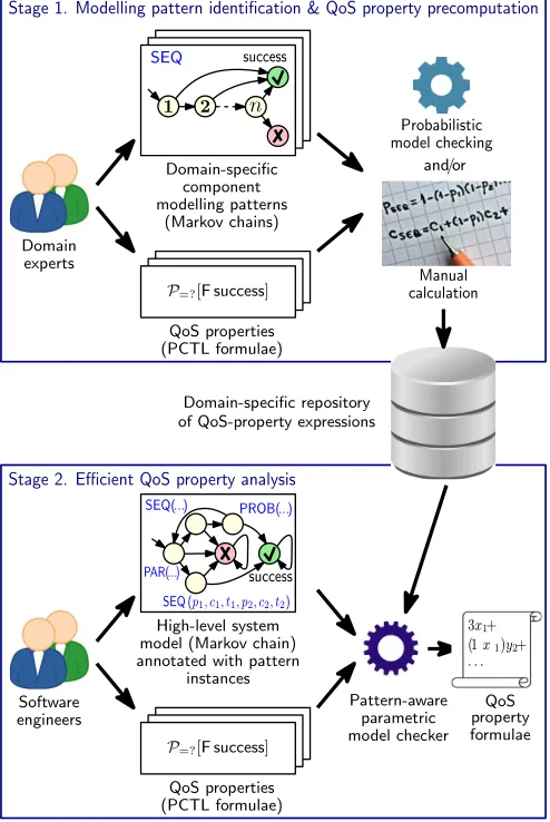
As shown in Fig. 1, ePMC comprises two stages. The first stage is performed only once for each domain that ePMC is applied to. This stage uses domain-expert input to identify modelling patterns for components of systems from the con-sidered domain, and precomputes closed-form expressions for key QoS properties of these patterns. For example, the modelling patterns for the service-based systems domain (described in detail in Section 6) correspond to different ways in which n ≥ 1 functionally-equivalent services can be used to execute an operation of the system. One option is to invoke the nservices sequentially, such that service 1 is always invoked, and servicei >1 is only invoked if the invocations of services 1, 2, . . . ,i−1have all failed. The com-ponent modelling pattern labelled ‘SEQ’ at the top of Fig. 1 depicts this option. The graphical representation of the pat-tern shows the invocations of thenservices as states labelled 1,2, . . . ,n, and the successful and failed completion of the operation as states labelled with a tick ’3_{’ and a cross ’}7_’, respectively. QoS properties such as the probability of reach-ing the success state and the expected execution time and cost of the operation for this pattern can be computed as

prob=p1+ (1−p1)p2+. . .+ Qni=1−1(1−pi)

pn

time=t1+ (1−p1)t2+. . .+ Qni=1−1(1−pi)

Domain-specific component modelling patterns

(Markov chains)

QoS properties (PCTL formulae)

P_=?[F success]

Domain experts

SEQ

QoS properties (PCTL formulae)

P_=?[F success]

Software engineers

High-level system model (Markov chain) annotated with pattern

instances

Pattern-aware parametric model checker

Probabilistic model checking

QoS property formulae

3x1+

(1x1)y2+ · · ·

Domain-specific repository of QoS-property expressions

Stage 2. Efficient QoS property analysis

Stage 1. Modelling pattern identi_fication & QoS property precomputation

success

SEQ(...)

SEQ (p1; c1; t1; p2; c2; t2) PROB(...)

PAR(...)

Manual calculation

and/or success

n

1 2

Fig. 1. Two-stage efficient parametric model checking

cost =c1+ (1−p1)c2+. . .+ Qni=1−1(1−pi)

cn

wherepi,tiandci are the probability of successful invoca-tion, the execution time and the cost of servicei,1≤i≤n, respectively. As illustrated in Fig. 1, these calculations can be carried out using an existing probabilistic model checker or manually. The resulting expressions are stored in a domain-specific repository, and are used in the next ePMC stage.

The second ePMC stage is performed for each struc-turally different variant of a system and QoS property under analysis. The stage involves the PMC of a parametric Markov chain that models the interactions between the system components. This Markov model can be provided by software engineers with PMC expertise, or can be generated from more general software models, such as UML activity diagrams annotated with probabilities as in [7], [18], [25]. The model states associated with system components are labelled with pattern instances that specify the modelling pattern used for each component and its parameters. For instance, the pattern instanceSEQ(p1, c1, t1, p2, c2, t2)from Fig. 1 labels a component implemented using the sequential pattern described earlier and n = 2 services with success probabilities p1, p2, costs c1, c2 and mean execution times

t1, t2. The pattern-annotated Markov model is analysed by a model checker with pattern manipulation capabilities. The

result of the analysis is a set of formulae comprising:

• A formula for the system-level QoS property, specified as a function over the component-level QoS property values. This formula is obtained by applying standard PMC to the pattern-annotated Markov model;

• Formulae for the relevant component-level QoS prop-erties. These formulae are obtained by instantiating the appropriate closed-form expressions from the domain-specific repository produced in the first ePMC stage. All ePMC formulae are rational functions that can be effi-ciently evaluated for any combinations of parameter values, e.g., using tools such as Matlab and Octave.

The main contributions of our paper are: 1) A theoretical foundation for the ePMC method.

2) An open-source tool that automates the application of the method, and is freely available from our project website https://www.cs.york.ac.uk/tasp/ePMC/. 3) Repositories of modelling patterns for the service-based

systems and multi-tier software architecture domains. 4) An extensive evaluation which shows that ePMC is

several orders of magnitude faster and produces much smaller algebraic expressions compared to the PMC techniques currently implemented by the leading model checkers PARAM, PRISM and Storm, in addition to supporting the analysis of parametric Markov chains that are too large for these model checkers.

These contributions build on our preliminary work from [12], extending it with a theoretical foundation, tool support, repositories of modelling patterns for two domains, and a significantly larger evaluation.

The rest of the paper is structured as follows. Section 2 provides a brief introduction to the model checking of para-metric Markov chains. Section 3 describes a simple service-based system that we then use as a running example when presenting the ePMC theoretical foundation in Section 4. Section 5 covers the implementation of the ePMC tool, while Sections 6 and 7 detail the application of ePMC to the service-based systems and multi-tier software architectures domains, respectively. Section 8 presents our experimental results, and Section 9 compares our method with related work. Finally, Section 10 provides a brief summary and discusses our plans for future work.

2

P

2.1 Parametric Markov chains

Markov chains(MCs) are finite state transition systems used to model the stochastic behaviour of real-world systems. MC states correspond to relevant configurations of the modelled system, and are labelled with atomic proposi-tions which hold in those states. State transiproposi-tions model all possible transitions between states, and are annotated with probabilities as specified by the following definition.

Definition 1. A Markov chain M over a set of atomic

propositionsAP is a tuple

M = (S, s0,P, L), (1)

where, for any statess, s′ _{∈S,P(s, s}′_{)is the probability of}

transitioning to statesfrom states′_{; andL:S→2}AP_{is the}

state labelling function.

A state s of a Markov chain M is anabsorbing state if P(s, s) = 1andP(s, s′_{) = 0for alls}′_{6=s, and atransient state}

otherwise. ApathπoverM is a possibly infinite sequence of states fromS such that for any adjacent statessand s′

in π,P(s, s′_{) > 0. Them-th state on a path π,m ≥ 1, is}

denotedπ(m). For any states,PathsM(s)represents the set of all infinite paths over M that start with states. Finally, we assume that every state s ∈ S is reachable from the initial state, i.e., there exists a pathπ∈PathsM(s0)such that

π(i) =sfor somei >0.

To compute the probability that a Markov chain (1) be-haves in a specified way when in states, we use aprobability measurePrsdefined overPathsM(s)such that [3], [37]:

Prs({π∈PathsM(s)|π=s1s2. . . sm. . .}) = P(s1s2. . . sm) =Qmi=1−1P(si, si+1),

where{π∈PathsM |π=s1s2. . . sm. . .}is the set of all in-finite paths that start with the prefix s1s2. . . sm (i.e., the

cylinder setof this prefix). Further details about this proba-bility measure and its properties are available from [3], [37]. To allow the verification of a broader set of QoS prop-erties, MC states can be annotated with nonnegative values termedrewards[2]. These values are interpreted as “costs” (e.g. energy used) or ”gains” (e.g. requests processed).

Definition 2. Areward structureover a Markov chainM =

(S, s0,P, L)is a functionρ:S →R≥0. For any states∈S, ρ(s)represents the reward “earned” on leaving states.

Our work focuses on the analysis of parametric Markov chains (sometimes called incomplete Markov chains [5] or

uncertain Markov chains[40]).

Definition 3. Aparametric Markov chainis an MC comprising

transition probabilitiesP(s, s′_{)and/or rewardsρ(s)defined}

as rational functions over a set of continuous variables [19], [32], [34].

2.2 Property specification

The properties of Markov chains are formally expressed in probabilistic variants of temporal logic. In our work we use probabilistic computation tree logic (PCTL) [17], [33] extended with rewards [2], which is supported by all leading probabilistic model checkers. Rewards-extended PCTL allows the specification of probabilistic and reward properties using the probabilistic operator P⊲⊳p[·] and the reward operatorR⊲⊳r[·], respectively, where p ∈ [0,1]is a probability bound, r ∈ R_{≥0 is a reward bound, and ⊲⊳∈} {≥, >, <,≤}is a relational operator. Formally, astate formula

Φand apath formulaΨin PCTL are defined by the grammar:

Φ ::=true|a|Φ∧Φ| ¬Φ| P⊲⊳p[Ψ] (2)

Ψ ::=XΦ|Φ U Φ|Φ U≤kΦ (3)

and areward state formulais defined by the grammar:

Φ ::=R⊲⊳r[I=k]| R⊲⊳r[C≤k]| R⊲⊳r[F Φ]| R⊲⊳r[S], (4)

wherek∈N_{>0is a timestep bound anda∈AP is an atomic} proposition. When multiple reward structures are defined

over a Markov chain, the extended notation Rrwd ⊲⊳r[I=k], Rrwd

⊲⊳r[C≤k], etc. is used to specify that a reward state formula

refers to the reward structure named ‘rwd’.

The PCTL semantics is defined using a satisfaction rela-tion|=over the statesS and the pathsPathsM(s),s ∈ S, of a Markov chain (1). Given a statesand a pathπ of the Markov chain,s |= Φmeans “Φholds in state s”,π |= Ψ means “Ψholds for pathπ”, and we have:

– s|=truefor alls∈S; – s|=aiffa∈L(s); – s|=¬Φiff¬(s|= Φ);

– s|= Φ1∧Φ2iffs|= Φ1ands|= Φ2;

– s|=P⊲⊳p[Ψ]iffPrs({π∈PathsM(s)|π|= Ψ})⊲⊳ p.

– thenext path formulaXΦholds for pathπiffπ(2)|= Φ; – the time-bounded until path formulaΦ1U≤kΦ2 holds for

pathπiffΦ2 holds in thei-th path state,i≤k, and Φ1 holds in the firsti−1path states, i.e.:

∃i≤k.(π(i)|= Φ2∧ ∀j < i.π(j)|= Φ1).

– theunbounded until formulaΦ1U Φ2removes the bound

kfrom the time-bounded “until” formula.

The notationF Φ≡trueU Φis used when the first part of an until formula istrue. Thus, thereachability propertyP⊲⊳p[F Φ] holds if the probability of reaching a state whereΦis true satisfies⊲⊳ p. Finally, the reward state formulae specify the expected values for: theinstantaneous rewardat timestepk,

R⊲⊳r[I=k_{]; thecumulative rewardup to timestepk,R⊲⊳r[C}≤k_];

thereachability rewardcumulated until reaching a state that satisfies a propertyΦ,R⊲⊳r[F Φ]; and thesteady-state reward

in the long run, R⊲⊳r[S]. For a detailed description of the PCTL semantics, see [2], [17], [33].

2.3 Parametric model checking

Probabilistic model checkers including MRMC [36], PRISM [38] and Storm [21] support the verification of PCTL proper-ties of Markov chains. To verify whether a formulaP⊲⊳p[Ψ] holds in a states, these tools first compute the probabilityp′

thatΨholds for MC paths starting ats, and then comparep′

to the boundp. The actual probabilityp′_{can also be returned}

(for the outermost operatorP of a formula) so PCTL was extended to include the formulaP=?[Ψ]denoting this prob-ability. Likewise, the extended-PCTL formulae R=?[I=k],

R=?[C≤k],R=?[F Φ], andR=?[S]denote the actual values of the expected rewards from (4).

Parametric model checking(PMC) represents the verifica-tion of quantitative PCTL properties P=?[.] without nested probabilistic operators and reward properties R=?[.] of parametric Markov chains using algorithms such as [19], [32], [34]. The PMC verification result is a rational function of the variables used to define the transition probabilities of the verified parametric Markov chain. PMC is supported by verification tools including the dedicated model checker PARAM [31], the latest versions of PRISM [38], and the recently released model checker Storm [21].

3

R

E

result₍op3)

false

y

true

1−y

Operation op1

Operation op2 result(op1) Operation op3

true

x

false

1−x

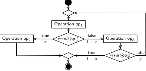
Fig. 2. UML activity diagram of the system used as a running example

implements the simple workflow from Fig. 2. This workflow handles user requests by first performing an operationop1. Depending on the result ofop1, its execution is followed by the execution of either operationop₂or operationop₃. The execution ofop₂completes the workflow, while after the ex-ecution ofop3the workflow may terminate or may need to re-executeop₁. The outgoing branches of the decision nodes from Fig. 2 are annotated with their unknown probabilities of execution (xand1−x, andyand1−y).

We suppose that multiple functionally-equivalent ser-vicessvci1,svci2, . . . can be used to perform each operation op_i,i∈ {1,2,3}, and that these services have probabilities of successful invocationpi1, pi2, . . ., expected response times

ti1, ti2, . . .and invocation costsci1, ci2, . . .Accordingly, the workflow can be implemented using different system ar-chitectures and service combinations. Our running example considers the implementation where:

• Operation op1 is executed by invoking services svc11 and svc12 sequentially, such that service svc11 is always invoked, and servicesvc12is only invoked if the invoca-tion ofsvc11fails (i.e., times out or returns an error). As a result, the operation completes successfully whenever either service invocation is successful, and fails when the invocations of both services fail.

• Operationop₂is executed using servicessvc21andsvc22

probabilistically, such thatsvc2j is invoked with

probabil-ityαjforj∈ {1,2}, whereα1+α2= 1.

• Operationop3is executed by invoking servicessvc31and svc32 sequentially with retry. This involves invoking the two services sequentially (as forop₁) and, if both service invocations fail, retrying the execution of the operation by using the same strategy with probabilityr∈(0,1). The parametric Markov chain from Fig. 3a models this implementation of the workflow. For instance, the MC states

s0 ands1 (labelled ‘op1’) model the execution of operation op1 by first invoking servicesvc11 (states0) and, if service servicesvc11fails (which happens with probability1−p11), also invokingsvc12 (state s1). The invocation of svc12 fails with probability1−p12, in which case the system transitions to state s3 and then to the ‘fail’ state s13. If either svc11 or svc12 succeeds (state s2), there is a probability x that operationop₂ (modelled by statess4–s8) is executed next, and a probability 1 −x that the next operation is op3 (modelled by statess9–s12).

To model the execution of operation op₂, the MC in-cludes transitions with probabilitiesα1 and α2 from s4 to

state s5 (which corresponds to the invocation of service svc21) and to states6 (which corresponds to the invocation of service svc22), respectively. The successful execution of svc21 or svc22 results in state s7 being reached and in the successful completion of the workflow (state s14, labelled ‘succ’), while a failed invocation results in state s8 being reached and in the failure of the workflow (states13). States

s9–s12 model the execution of operation op3 similarly to howop₁is modelled bys0–s3, except that a successful exe-cution ofop3is followed byop1(with probabilityy) or the successful end of the workflow (with probability1−y), and failed invocations ofsvc32 lead to a retry of the operation (with probabilityr) or to the failure ofop3 and thus of the entire workflow (with probability1−r). Finally, two reward structures are defined in Fig. 3a. These structures, named ‘time’ and ’cost’, map the MC states associated with service invocations to the expected execution time and the cost of these services, respectively.

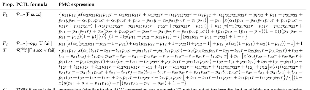
Parametric model checking applied to the MC from Fig. 3a can compute closed-form expressions for a wide range of QoS properties of the system. These properties can then be evaluated very efficiently for different combinations of services with different parameters. For our running example, we assume that the software engineers developing the system are interested to analyse the following properties: (i) The probabilityP1that the workflow implemented

by the system completes successfully;

(ii) The probabilityP2that the workflow fails due to a failed execution of operationsop₁orop₂;

(iii) The expected execution timeT of the workflow; (iv) The expected costCof executing the workflow.

Table 1 presents these properties formalised in PCTL, and their closed-form expressions computed using the proba-bilistic model checker Storm and significantly simplified through manual factorisation. These results, included in order to show how large and complex the PMC expressions can be even for a simple model, already suggest that PMC might not be feasible for larger systems and models. The experimental results presented later in Section 8 confirm that indeed the PMC techniques implemented by current model checkers do not scale to much larger systems than the one from Fig. 2—a limitation addressed by our ePMC method described next.

4

PMC T

F

a. Parametric Markov chain model of the workflow implementation under analysis, with shaded fragmentsF1(corresponding to operation

op1), F2 (corresponding to op2) and F3 (corresponding to op3). The `tijjcij' combinations annotating the states that model service

invocations define `time' and `cost' reward structures for analysing the expected executiontime _andcost _{of the workflow, respectively.}

1 1

s13 s14

fail succ

1

1 1 1

1−y

y

x

1−x

1

b. Parametric Markov chains associated with fragmentsF1{F3from Fig. 3a

e1

1

e2

1

e3

e1 e2 e3

z1 op1

1

1

z2

s13 s14

fail succ

z1 op1

op2

z3 op3

(1−prob3)(1−y) prob2

1−prob2

(1−prob3)y prob3

(i) (ii)

c. Abstract Markov chains induced by (i) fragmentF1, and (ii) fragmentsF1{F3of the parametric Markov chain from Fig. 3a

1 1

s13 s14

fail succ

1

1

1

1−y

y

prob1x

prob1(1−x)

1−prob1 time1jcost1

prob1x

prob1(1−x)

1−prob1 time1jcost1

time2jcost2

time3jcost3

Fig. 3. ePMC application to a parametric Markov chain model of the workflow from the running example

TABLE 1

Parametric model checking of the four QoS properties from the running example

Prop. PCTL formula PMC expression

P1 P=?[F succ]

p11p12x(α2p31p22p32r−α1p31p21r+α1p21r−α1p21p32r−α2p22+α1p31p21p32r−yp32+p31−p31p32+

p31yp32−α2p22p32r+α2p22r+p32−p31y−α2p31p22r−α1p21)+p11x(α1(p21−p31p21p32r+p21p32r−

p21r+p31p21r) +α2(p31p22r−p31p22p32r−p22r+p22p32r+p22))+p12x(α1(p21p32r−p21r−p31p21p32r+

p21+p31p21r) +α2(p22+p22p32r−p22r+p31p22r−p31p22p32r)) + (p11p12−(p11+p12)(1−x))(p31p32−

p31−p32)(1−y) /(1−x)y(p11+p12−p12p12)−r(p31p32−p31−p32) + 1−r

P2 P=?[¬op3Ufail] p11x(α1(p12p21−p12+ 1−p21) +α2(p12p22−p12+ 1−p22)) +p12−1+p12x(α1(1−p21) +α2(1−p22))−1+ 1

T Rtime

=?[F succ∨fail]

p11p12x(α1(t21r−t21−t21p32r−p31t21r+p31t21p32r) +α2(p31t22p32r−t22+t22r−t22p32r−p31t22r) +t32+

t31−p31t32) +t12p31p32r−t32−t31+p31t32−t12+t12r−t12p32r−t12p31r+p11x(α2(t22−t22r+t22p32r+

p31t22r−p31t22p32r) +α1(t21−t21r+t21p32r+p31t21r−p31t21p32r)−t32−t31+p31t32) +t32+t31−p31t32−

t12r+t12p32r+t12p31r−t12p31p32r−t11+t11r−t11p32r−t11p31r+t11p31p32r+t12+p12x(α1(t21p32r+

p31t21r−p31t21p32r+t21−t21r) +α2(t22−t22r+t22p32r+p31t22r−p31t22p32r)−t32−t31+p31t32) +t31−

p31t32+t32+t12−t12r+t12p32r+t12p31r−t12p31p32r+t11−t11r+t11p32r+t11p31r−t11p31p32r /(1−

x)y(p11+p12−p11p12)−r(p31p32−p31−p32) + 1−r

C Rcost

outgoing transition probabilities and rewards of the new state can be obtained through the analysis of a parametric MC associated with the fragment, where the size of this MC is similar to that of the fragment. We formally define these concepts below.

Definition 4. Afragmentof a parametric Markov chainM =

(S, s0,P, L)is a tupleF = (Z, z0, Zout),where: - Z ⊂Sis a subset of transient MC states;

- z0 is the (only)entry stateofF, i.e.,{z0}={z∈Z | ∃s∈

S\Z .P(s, z)>0};

- Zout = {z ∈ Z | ∃s ∈ S \ Z .P(z, s) > 0} is the non-empty set of output states of F, and all outgoing transitions from the output states are to states outside

Z, i.e.,P(z, z′_{) = 0for all(z, z}′_)∈Z out×Z.

According to this definition, the output states of a fragment cannot have outgoing transitions to other states within the same fragment. However, a simple model transformation can be used to form a fragment from a state set Z that includes states z with outgoing transitions to states both inside and outside Z. This transformation replaces each such state z with states z′ _{and z}′′ _{such that: z}′ _{“inherits”}

all incoming transitions of z and its outgoing transitions to states within Z, and has an additional outgoing tran-sition to z′′ _{(with transition probability calculated so that}

the transition probabilities of z′ _{add up to 1.0); and z}′′

only has the incoming transition from z′_{, and inherits the}

output transitions fromzto states outsideZ(with transition probabilities scaled to add up to1.0).

Example 1. The shaded areas of the parametric MC from

Fig. 3a (each corresponding to an operation of the workflow from our running example) contain three MC fragments:

F1= ({s0, s1, s2, s3}, s0,{s2, s3})

F2= ({s4, s5, s6, s7, s8}, s4,{s7, s8})

F3= ({s9, s10, s11, s12}, s9,{s11, s12})

As shown by this example, MC fragments may or may not contain cycles.

Given a fragmentF of a parametric MCM, ePMC per-forms parametric model checking by separately analysing two parametric MCs determined byF, and combining the results of the two analyses. As each of the two parametric MCs has fewer states and transitions than M, the overall result can be obtained in a fraction of the time required to analyse the original modelM. The first of these parametric MCs is defined below.

Definition 5. The Markov chain associated with a fragment

F = (Z, z0, Zout)of a parametric MC M = (S, s0,P, L) is the Markov chainMZ= (Z ∪ {e}, z0,PZ, LZ), wheree is

an additional, “end” state, the transition probability matrix PZ : (Z∪ {e})×(Z∪ {e})→[0,1]is given by

PZ(z, z′) =   

1, ifz∈Zout∪ {e} ∧z′ =e P(z, z′_{), ifz∈Z\Z}

out∧z′6=e 0, otherwise

,

and the atomic propositions for statez∈Zare given by

LZ(z) =   

L(z)∪ {z}, ifz∈Zout {e}, ifz=e L(z), otherwise

,

where z and e are atomic propositions that hold in state

z∈Zoutand statee, respectively.1Additionally, any reward structureρ:S→R_{≥0 over M naturally maps to a reward} structureρZ:Z∪ {e} →R_{≥0 over MZ, where ρZ(e) = 0} and, for allz∈Z,ρZ(z) =ρ(z).

Example 2. Fig. 3b shows the parametric MCs associated

with fragmentsF1–F3from Example 1, obtained by: (i) adding transitions of probability 1 from the output states

inZout1={s2, s3},Zout2={s7, s8}andZout3={s11, s12} to additional statese1,e2ande3, respectively;

(ii) labelling the output states with the additional atomic propositions s2 ands3,s7 ands8, ands11 ands12, and the end states with the new atomic propositionse1toe3.

The second parametric MC determined by a fragmentF

and analysed by ePMC is obtained from the original MC by replacing all states fromF with a single state.

Definition 6. Given a fragment F = (Z, z0, Zout) of a

parametric Markov chainM= (S, s0,P, L), theabstract MC

induced byF isM′_{= (S}′_{, s}′

0,P′, L′),where:

- The state setS′ _{= (S\Z)∪{z}, wherezis a new,abstract} statethat stands for all the states fromZ;

- The initial states′

0 =s0, ifs0is not the initial state ofZ (i.e.,z06=s0), ands′0=zotherwise;

- The transition probability between statess, s′_∈S′_is

P′(s, s′) =         

P(s, s′_{), ifs6=z∧s}′_6=z P(_Ps, z0), ifs6=z∧s′=z

z∈Zout

prob_z·P(z, s′_{), ifs=z∧s}′_6=z

0, otherwise

where

probz=P=?[Fz] (5)

is a reachability property calculated over the parametric Markov chain associated with the fragment F, for all output statesz∈Zout;2

- The labelling functionL′ _{coincides withLfor the states}

from the original MC, and maps the new statez to the (potentially empty) set of atomic propositions common to all states fromF,3

L′(s) = (

L_T(s) ifs∈S\Z

z∈Z

L(z) otherwise (i.e. ifs=z)

Finally, for every reward structure defined over the Markov chain M, state z from the induced Markov chain is anno-tated with a reward

rwd =Rrwd

=? [Fe] (6)

1. As shown later in this section, these new atomic propositions allow the computation of the reachability probabilitiesP=?[Fz]for the states

z ∈ Zout and of the reachability reward Rrwd_=?[Fe]for any reward structurerwddefined overF.

2. Note thatPs′_∈S′P′(z, s′) = P

s′_∈S\Z P

z∈ZoutprobzP(z, s

′_{) =}

P

z∈Zoutprobz P

s′_∈

S\ZP(z, s′) = P

z∈Zoutprobz·1 =P=?[F W

z∈Zoutz]

= 1as required.

3. Since the occurrence ofzon a path of the abstract MC stands for

calculated over the parametric MCMZ associated withF. Thus, rwd represents the cumulative reward to reach the end state ofMZ.

Example 3. Consider again the parametric Markov chain

from our running example (Fig. 3a). The corresponding ab-stract MC induced by fragmentF1from Example 1 is shown in Fig. 3c(i). This abstract MC is obtained by replacing all the states fromF1with the single abstract statez1, and by using the rules from Definition 6 to find the outgoing transition probabilities and atomic propositions for z1. For example, the transition probability fromz1tos4is calculated as:

P′(z1, s4) =

X

z∈{s2,s3}

probz·P(z, s4)

=prob_s2·P(s2, s4) +probs3·P(s3, s4) =probs2·x+probs3·0

=prob_s2·x,

whereprob_s2=P=?[Fs2]andprobs3=P=?[Fs3] = 1−probs2 are reachability properties calculated over the parametric MC associated with fragment F1 (cf. Fig. 3b). As the two output-state reachability probabilities (5) for fragment F1 can be expressed in terms of a single probability, we use the notationprob1=probs2for this probability in Fig. 3c(i). The transition probabilities fromz1tos9ands13are calculated similarly, and the transition probability from s12 to z1 is simply P′(s12, z1) = P(s12, s0) = y (since the entry state of F1 is s0). All other transition probabilities from z1 to other states and from other states toz1 are zero. Statez1is labelled with the atomic propositionop1, which is the only label common to all states from the fragmentF1. Finally,z1 is annotated with the rewardstime1=Rtime=? [Fs2∨s3]and

cost1=Rcost=?[Fs2∨s3]computed over the parametric MC associated withF1.

Fig. 3c(ii) shows the abstract Markov chain obtained after all three fragments F1–F3 from Example 1 were used to simplify the initial MC from Fig. 3a. Note how even for the small MC from our running example, the abstract MC from Fig. 3c(ii) is much simpler than the initial MC from Fig. 3a; the abstract MC has only 5 states and 10 transitions, compared to 15 states and 25 transitions for the initial MC.

The ePMC computation of unbounded until proper-tiesP=?[Φ1U Φ2] (and thus also of reachability properties

P=?[F Φ] =P=?[trueU Φ]) is based on the following result.4

Theorem 1. Let F be a fragment of a parametric Markov

chainM, andΦ1andΦ2two PCTL state formulae overM. If every atomic propositionapthat appears inΦ1orΦ2either holds in every fragment statez(i.e.,ap ∈L(z)) or holds in no such state,5 _{then the PMC of the until PCTL formula} P=?[Φ1U Φ2] over M yields an expression equivalent to that produced by the PMC of the formula over the abstract Markov chain induced byF.

4. The computation of bounded until properties is not supported be-cause path lengths are not preserved by the ePMC abstraction process. 5. While this requirement restricts the state formulae that the the-orem applies to (or, alternatively, the fragments that can be usefully constructed), the evaluation presented later in the paper shows that the theorem supports the efficient analysis of multiple properties of practical relevance.

Proof. Let A, A′ _{be the sets of paths that satisfy the PCTL}

formulaΦ1U Φ2for the MCM(S, s0,P, L)and for the MC

M′_(S′_{, s}′

0,P′, L′)induced byF(Z, z0, Zout):

A={π∈PathsM(s0)| ∃i >0.(π(i)|= Φ2 ∧ ∀j < i.π(j)|= Φ1)}

A′={π′∈PathsM′(s′0)| ∃i >0.(π′(i)|= Φ2∧ ∀j < i.π′(j)|= Φ1)}

According to the semantics of PCTL (cf. Section 2.2), we need to show that Prs0(A) = Pr

′ s′

0(A

′_{), where Pr} s0 and Pr′s′

0are probability measures defined overPaths M_(s

0)and

PathsM ′

(s′

0), respectively, as explained in Section 2.1. A path

π∈Ahas the general form

π=π0ω1π1ω2π2. . . ωnπn. . . , (7)

where π0, π1, . . . , πn are subpaths comprising only states from S \ Z, ω1, ω2, . . . , ωn are subpaths comprising only states fromZ, and the first state ofπthat satisfiesΦ2is the last state from the path prefix π0ω1π1ω2π2. . . ωnπn. Note that (7) subsumes the scenarios when the path prefix starts with a state fromZ (subpathπ0 empty), ends with a state fromZ(subpathπnempty), contains only states fromS\Z

(n= 0), or contains only states fromZ(n= 1, and subpaths

π0andπ1empty). We have three cases.

Case 1)Ifn > 0andπn is non-empty, the subpathsω1,

ω2, . . . ,ωn must all start withz0 and end with a statez ∈

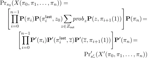
Zout (as paths can only “enter” and “exit” MC fragments through their only entry state and one of their output states, respectively). Furthermore,z0 andzmust satisfyΦ1 (since it belongs to the prefix of pathπ), so all states fromZ also satisfy Φ1 (as required by the theorem). This means that substituting any subset ofω1,ω2, . . . ,ωn from πwith any combination of fragment subpaths starting atz0and ending with a state fromZout changesπinto a sequence of states that either belongs toA(if it is a path fromPathsM(s0)) or has probability 0 of occurring inM (otherwise). Given the set of all pathsX(π0, π1, . . . , πn)⊆Athat can be obtained through such substitutions, and using the notationπlast

i for

the last state on subpathπi,1≤i≤n, we have:

Prs0(X(π0, π1, . . . , πn)) =

 

n_Y−1

i=0

P(πi)P(πlasti , z0)

X

z∈Zout

prob_zP(z, πi+1(1))



P(πn) =

"_n−1 Y

i=0

P′(πi)P′(πlast

i , z)P′(z, πi+1(1))

#

P′(πn) =

Pr′s′

0(X

′_(π

0, π1, . . . , πn))

whereX′_(π

0, π1, . . . , πn) = {π′∈PathsM

′

(s′

0)|π′ =π0zπ1

zπ2. . . zπn. . .} ⊆ A′ (since all states π0, π1, . . . , πn andz satisfyΦ1, andπlast

n satisfiesΦ2). We can similarly show that

any subsetX′_(π

0, π1, . . . , πn)ofA′ with paths of the form

π0zπ1 zπ2. . . zπn. . . and on which Φ2 first holds in state

πlast

n corresponds to a subset X(π0, π1, . . . , πn) ⊆ A such thatPr′s′

0(X

′_(π

0, π1, . . . , πn)) = Prs0(X(π0, π1, . . . , πn)).

Case 2)Ifn >0andπnis empty, then the last state ofωn

states fromω1and its initial state,z0, so the set of pathsπ form the setX(π0) ={π∈PathsM(s0)|π=π0z0. . .} ⊆A, and we have:

Prs0(X(π0)) =P(π0)P(πlast0 , z0) =

P′(π0)P′(πlast0 , z) = Pr′s′

0(X

′_(π

0)),

where X′_(π

0) = {π′∈PathsM

′

(s′

0)|π′ = π0z . . .} ⊆ A′. In a similar way, we can show that any subsetA′_(π

0)ofA′ with paths of the formπoz . . .and on whichΦ2first holds in state z corresponds to a subset X(π0) of A such that Pr′s′

0(X

′_(π

0)) = Prs0(X(π0)).

Case 3)Finally, ifn= 0, the pathπfrom (7) becomesπ= π0. . ., and equiprobable setsX(π0)⊆AandX′(π0)⊆A′ are straightforward to identify.

We have shown that A and A′ can be partitioned into pairs of corresponding subsetsX ⊆AandX′_⊆A′_{that are}

equiprobable according to the probability metricsPrs0 and Pr′_s′

0, which completes the proof.

The repeated application of Theorem 1 reduces the com-putation of until properties P=?[Φ1U Φ2] of a parametric MC with multiple fragmentsF1,F2, . . . to computing:

1) the output-state reachability probabilities for the para-metric MCs associated withF1,F2, . . . ;

2) P=?[Φ1U Φ2] for the parametric MC induced by the fragments,

and combining the results from the two ePMC stages into a set of algebraic formulae over the parameters of the original MC. The parametric MCs from these stages are typically much simpler than the original, “monolithic” MC, and much faster to analyse. In addition, ePMC focuses on frequently used domain-specific fragmentsF1,F2, . . . , and thus stage 1 only needs to be executed once for a domain. Note that a result similar to Theorem 1 is not available for bounded until properties P=?[Φ1U≤kΦ2] because the abstract MC induced by a set of fragmentsF1, F2, . . .does not preserve the path lengths from the original MCs.

Example 4. We use the above two-stage method to compute

propertiesP1andP2from our running example (cf. Table 1). In stage 1 we compute the output-state reachability prop-erties for the parametric MCs associated with fragmentsF1–

F3(cf. Fig. 3b):

• for the MC associated withF1,prob1=p11+(1−p11)p12;

• for the MC associated withF2,prob2=α1p21+α2p22;

• for the MC associated withF3,prob₃= (p31+ (1−p31)

p32)/(1−(1−p31)(1−p32)r).

We computed these algebraic expressions manually, based on the MCs from Fig. 3b. However, they can also be obtained using one of the model checkers mentioned earlier (i.e., PARAM, PRISM and Storm), or can be taken directly from our ePMC repository of such expressions for the service-based systems domain (see Section 6 later in the paper).

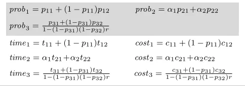
In stage 2, we use a probabilistic model checker (we used Storm) to computeP1 andP2 over the induced parametric MC from Fig. 3c. The shaded formulae from Table 2 show the expressions obtained for P1 and P2, preceded by the results from the first ePMC stage.

TABLE 2

ePMC of the QoS properties from the running example

Output-state reachability formulae computed in stage 1 of ePMC

prob₁=p11+ (1−p11)p12 prob2=α1p21+α2p22

prob₃= p31+(1−p31)p32

1−(1−p31)(1−p32)r

time1=t11+ (1−p11)t12 cost1=c11+ (1−p11)c12

time2=α1t21+α2t22 cost2=α1c21+α2c22

time3=₁₋₍₁₋t31+(1−p31)(1−p31)pt3232)r cost3=

c31+(1−p31)c32

1−(1−p31)(1−p32)r

Property-specific formulae computed in stage 2 of ePMC

Prop. PCTL formula ePMC set of formulae

P1

P2

T

C

P=?[F succ]

P=?[¬op3Ufail]

Rtime

=?[F succ∨fail]

Rcost

=?[F succ∨fail]

P1=prob1(₁₋₍₁₋xprob2_x+(1−_)yprobx)(1−y)prob3)

1prob3 P2= 1−prob1+xprob1(1−prob2)

T =time1+prob1(xtime2+(1−x)time3)

1−(1−x)yprob1prob3

C =cost1+prob1(xcost2+(1−x)cost3)

1−(1−x)yprob1prob3

Expectedly, the set of formulae from Table 2 is much simpler than the “monolithic” P1 and P2 formulae from Table 1. As we will show in Section 8, this difference is even more significant for larger models, making the computation and evaluation of “monolithic” formulae challenging for existing PMC techniques.

The final result from this section allows the efficient para-metric model checking of reachability reward properties.

Theorem 2. Let F be a fragment of a parametric Markov

chain M, and T a set of states fromM. If T includes no state fromF, then the PMC of the reachability reward PCTL formulaR=?[FT]overM yields an expression equivalent to that produced by the PMC of the formula over the abstract MCM′_{induced byF.}

Proof. We adopt one of the alternative definitions for the reachability reward R=?[FT] from [3, §10.5.1]. Given the setAof all finite pathsπ =s0s1. . . sm fromM such that

sm∈Tands0, s1, . . . , sm−1∈/ T, we have:

R=?[FT] =

0, ifP<1[FT]

P

π∈AP(π)ρ(π), otherwise

(8)

whereρ(π) =Pm_i=0−1ρ(si).

According to Theorem 1, if P<1[FT] over M then

P<1[FT]overM′ too, soR=?[FT] = 0over both M and

M′_{and the theorem holds. The theorem also holds trivially}

whenAcontains no paths with states fromZ: in this case, it is straightforward to show that A is also the set of all finite paths s0s1. . . sm from M′ such that sm ∈ T and

T ∩Z = ∅ and Zout states are followed by a state from outsideZ). Thus, the generic form of such a path is

π= ∈S\Z z }| { s0. . . si

=z0 z}|{ si+1

∈Z z }| { si+2. . . sj−1

∈Zout

z}|{ sj

∈S\Z z}|{ sj+1

∈S

z }| {

sj+2. . . sm−1

| {z }

/ ∈T sm |{z} ∈T (9) We consider the subset of all paths A1 ⊆ A that start with the prefix s0. . . siz0 and, using the notation πx,y =

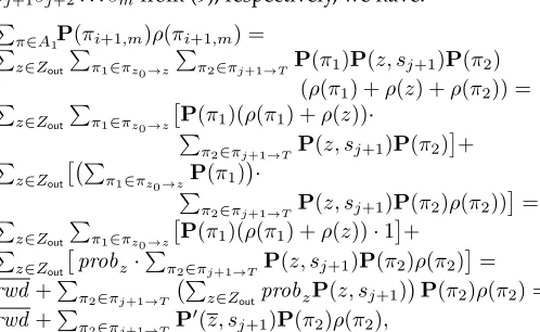
sxsx+1. . . sy, we calculate their contribution to the sum from the second row of (8):

C(s0, s1, . . . , si, z0) =Pπ∈A1P(π)ρ(π) = P

π∈A1P(π0,i+1)P(πi+1,m)(ρ(π0,i+1)+ρ(πi+1,m)) = P(π0,i+1) Pπ∈A1P(πi+1,m)

ρ(π0,i+1)+

P

π∈A1P(πi+1,m)ρ(πi+1,m)

= P(π0,i+1)1·ρ(π0,i+1) +Pπ∈A1P(πi+1,m)ρ(πi+1,m)

,

sinceP≥1[FT] requires thatPπ∈A1P(πi+1,m) = 1. Addi-tionally, using the shorthand notation πz0→z and πj+1→T for the set of all sub-paths si+1si+2. . . sj associated with a fixed sj = z ∈ Zout and for the set of all sub-paths sj+1sj+2. . . smfrom (9), respectively, we have:

P

π∈A1P(πi+1,m)ρ(πi+1,m) = P

z∈Zout

P

π1∈πz0→z P

π2∈πj+1→T P(π1)P(z, sj+1)P(π2) (ρ(π1) +ρ(z) +ρ(π2)) =

P z∈Zout

P

π1∈πz0→_z

P(π1)(ρ(π1) +ρ(z))·

P

π2∈πj+1→TP(z, sj+1)P(π2)

+ P

z∈Zout

P

π1∈πz0→zP(π1)

· P

π2∈πj+1→_TP(z, sj+1)P(π2)ρ(π2))

= P

z∈Zout

P

π1∈πz₀→z

P(π1)(ρ(π1) +ρ(z))·1+

P z∈Zout

probz· P

π2∈πj+1→T P(z, sj+1)P(π2)ρ(π2)

=

rwd+P_π2∈πj+1→T P

z∈ZoutprobzP(z, sj+1)

P(π2)ρ(π2) =

rwd+Pπ2∈πj+1→_T P ′_{(z, sj}

+1)P(π2)ρ(π2),

where rwd, probz and P′(z, sj+1) are those from Defini-tion 6, and where we used the fact thatP≥1[FT]to infer that

P

π2∈πj+1→TP(z, sj+1)P(π2) = 1 and to include all

non-zero-probability sub-paths at every step of the calculation. Combining the results so far, we obtain

C(s0, s1, . . . , si, z0) =P(_Pπ0,i+1) ρ(π0,i+1) +rwd +

π2∈πj+1→T P ′_{(z, sj}

+1)P(π2)ρ(π2)).

This reward “contribution” is equivalent to that obtained by replacing all sub-paths fromF appearing in paths from

A1 immediately after the prefix s0s1. . . si with state z comprising a reward valuerwd and transition probabilities P′(z, sj+1)to statessj+1∈S\Z. By repeating this process to replace all occurrences of sub-paths fromF appearing in

A, we obtain an expression equivalent toP_π∈AP(π)ρ(π), but corresponding to the parametric model checking of

R=?[FT] over the abstract MCM′ induced by F, which completes the proof.

The previous theorem reduces the computation of reach-ability reward propertiesR=?[FT]of a parametric MC with fragmentsF1,F2, . . . to computing:

1) the per-fragment cumulative reachability reward prop-erties for the MCs associated withF1,F2, . . . ;

2) R=?[FT]for the MC induced by these fragments,

and combining the results from the two stages into a set of algebraic formulae over the parameters of the original MC. Note that results similar to Theorem 2 are not available for instantaneous, cumulative and steady-state rewards formu-lae because the abstract MC induced byF1,F2, . . . does not preserve the path lengths and the rewards structures of the original MC.

Example 5. We use ePMC to calculate propertiestimeand

cost from our running example (cf. Table 1), starting with the cumulative reachability reward properties for fragments

F1–F3, i.e., ti and ci for i = 1,2,3. The resulting formu-lae, which we obtained manually (but which can also be obtained using a PMC tool) are shown in the top half of Table 2. For the second ePMC stage, we used the model checker Storm to obtain the algebraic expressions fortime

andcostfrom the lower half of Table 2.

As in Example 4, ePMC produced a set of formulae that is far simpler than the “monolithic” time and cost from Table 1. Note that we do not compare the analysis time of our ePMC method with that of existing PMC here or in Example 4 because for the simple system from our running example the two analysis times are similar. However, we do provide an extensive comparison of these analysis times for larger systems in our evaluation of ePMC from Section 8.

5

I

We developed a pattern-aware parametric model checker that implements the theoretical results from the previous section. This tool automates the second stage of ePMC. As shown in Fig. 1, the ePMC tool uses a domain-specific repository of QoS-property expressions to analyse PCTL-specified QoS properties of a parametric Markov chain annotated with pattern instances.

The domain-specific repository comprises entries with the general format:

pattern name ( p a r a m e t e r l i s t ) :

property name=expr , . . . , property name=expr ;

Each such entry defines algebraic expressions for the reach-ability properties and the reachreach-ability reward properties of a parametric MC fragment commonly used within the domain of interest, i.e., amodelling pattern.

Example 6. Table 3 shows a part of the ePMC repository

for the service-based systems domain. This part includes the three patterns used by the operations from our running example (SEQforop1,PROBforop2, andSEQ Rforop3), such that the formulae from the top half of Table 2 can be obtained (without any calculations) by instantiating the relevant patterns:

prob₁=SEQ(p11, c11, t11, p12, c12, t12).prob

prob2=PROB(α1, p21, c21, t21, α2, p22, c22, t22).prob

prob₃=SEQ R(p31, c31, t31, p32, c32, t32, r).prob

time1= SEQ(p11, c11, t11, p12, c12, t12).time

cost1= SEQ(p11, c11, t11, p12, c12, t12).cost

time2= PROB(α1, p21, c21, t21, α2, p22, c22, t22).time

cost2= PROB(α1, p21, c21, t21, α2, p22, c22, t22).cost

time3= SEQ R(p31, c31, t31, p32, c32, t32, r).time

cost3= SEQ R(p31, c31, t31, p32, c32, t32, r).cost

TABLE 3

Fragment of the ePMC repository of QoS-property expressions for the service-based systems domain, comprising expressions for the probability of pattern invocation successprob, expectedcost, and

expected executiontime

SEQ ( p1 , c1 , t1 , p2 , c2 , t 2 ) :

prob=p1+(1−p1 )∗p2 , c o s t =c1+c2∗(1−p1 ) , time= t 1 +(1−p1 )∗t 2 ;

. . .

PROB( x1 , p1 , c1 , t1 , x2 , p2 , c2 , t 2 ) : prob=x1∗p1+x2∗p2 , c o s t =x1∗c1+x2∗c2 , time=x1∗t 1 +x2∗t 2 ;

. . .

SEQ R ( p1 , c1 , t1 , p2 , c2 , t2 , r ) :

prob =( p1+(1−p1 )∗p2)/(1−(1−p1 )∗(1−p2 )∗r ) , c o s t =( c1 +(1−p1 )∗c2 )/(1−(1−p1 )∗(1−p2 )∗r ) , time =( t 1 +(1−p1 )∗t 2 )/(1−(1−p1 )∗(1−p2 )∗r ) ; . . .

The ePMC model checker supports the analysis of pattern-annotated parametric Markov chains specified in the PRISM high-level modelling language. This language models a system as the parallel composition of a set of

modules. The state of a module is encoded by a set of finite-range local variables, and its state transitions are defined by probabilistic guarded commands that change these variables, and have the general form:

[action]guard→e1:update1+ . . . +eN:updateN;

In this command, guard is a boolean expression over all model variables. If guard evaluates to true, the arithmetic expression ei, 1 ≤ i ≤ N, gives the probability with which the updatei change of the module variables occurs.

When the label action is present, all modules comprising commands with this action have to synchronise (i.e., can only carry out one of these commands simultaneously).

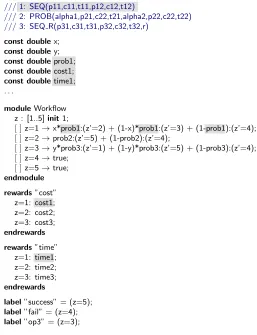
Example 7. Fig. 4 shows how the parametric MC from

Fig. 3c(ii) and its reward structures and labels are specified in this high-level modelling language. The valuesz= 1 to z = 5 of the local variable z from the Workflow module correspond to statesz1,z2,z3,s13ands14 from Fig. 3c(ii), respectively. The model parameters prob1 to prob3, cost1 tocost3andtime1to time3are associated with the pattern annotations from the lines starting with a triple forward slash ‘///’. These annotations tell the ePMC model checker that the model has parameters associated with QoS prop-erties of modelling patterns from the repository in Table 3. For example, the shaded pattern annotation at the top of Fig. 4 specifies that the QoS propertiesprob,costand time of theSEQmodelling pattern appear as parameters named prob1, cost1 and time1 in the model, where the id ‘1’ is provided before the pattern name. The occurrences of these parameters are also shaded in Fig. 4.

The general format of an ePMC pattern annotation is:

/// id : pattern name ( a c t u a l p a r a m e t e r l i s t )

This annotation indicates that some or all QoS properties of the pattern appear as parameters in the parametric MC, with the name of each such parameter obtained by appending the idfrom the annotation to the name of the QoS property.

/// 1: SEQ(p11,c11,t11,p12,c12,t12)

/// 2: PROB(alpha1,p21,c22,t21,alpha2,p22,c22,t22) /// 3: SEQ R(p31,c31,t31,p32,c32,t32,r)

const double_x;

const double_y;

const doubleprob1;

const doublecost1;

const doubletime1;

. . .

moduleWorkflow

z : [1..5]init1;

[ ]z=1!x*prob1:(z'=2) + (1-x)*prob1:(z'=3) + (1-prob1):(z'=4);

[ ]z=2!prob2:(z'=5) + (1-prob2):(z'=4);

[ ]z=3!y*prob3:(z'=1) + (1-y)*prob3:(z'=5) + (1-prob3):(z'=4);

[ ]z=4!_true;

[ ]z=5!true; endmodule

rewards_"cost" z=1: cost1; z=2: cost2; z=3: cost3; endrewards

rewards_"time" z=1: time1; z=2: time2; z=3: time3; endrewards

label_{"success" = (z=5);} label"fail" = (z=4); label"op3" = (z=3);

Fig. 4. Pattern-annotated parametric Markov chain for the service-based system from the running example

Given a domain-specific repository of QoS-property ex-pressions, a pattern-annotated parametric MC and a set of PCTL-encoded QoS properties, the ePMC model checker uses the theoretical results from Section 4 to compute a set of algebraic formulae comprising:

1. Formulae for every MC parameter associated with a modelling pattern listed in the model annotations. These formulae are obtained by instantiating the expressions from the repository, as shown in (10). The top half of Table 2 shows these formulae for the MC in Fig. 4. 2. A formula for each analysed QoS property, obtained by

applying standard parametric model checking, i.e., by ignoring the pattern annotations of the parametric MC. The bottom half of Table 2 shows these formulae for the four QoS properties from our running example.

The ePMC tool can be configured to use PRISM or Storm for the computation of the latter formulae, and outputs the combined set of algebraic formulae as a MATLAB file, ready for evaluation or further analysis with MATLAB.

6

PMC

S

-B

S

TABLE 4

Modelling patterns for the implementation of SBS operations usingnfunctionally-equivalent services

Pattern Description

SEQ(p1, c1, t1, . . . , pn, cn, tn) Thenservices are invoked in order, stopping after the first successful invocation or after the

last service.

PAR(p1, c1, t1, . . . , pn, cn, tn)† Thenservices are all invoked at the same time, and the operation uses the first result returned

by a successful invocation (if any).

PROB(x1, p1, c1, t1, . . . , xn, pn, cn, tn) A single service is invoked;xigives the probability that this is servicei, wherePni=1xi= 1.

SEQ R(p1, c1, t1, . . . , pn, cn, tn, r) The nservices are invoked in order as for theSEQ pattern; if all ninvocations fail, the

execution of the operation is retried (from service1) with probabilityror the operation fails with probability1−r.

SEQ R1(p1, c1, t1, r1, . . . , pn, cn, tn, rn) The services are invoked in order. If serviceifails, it is reinvoked with probabilityri; with

probability1−ri, the operation is attempted using servicei+ 1(ifi < n) or fails (ifi=n).

PAR R(p1, c1, t1, . . . , pn, cn, tn, r)† Allnservices are invoked as for thePARpattern; if allninvocations fail, the execution of the

operation is retried with probabilityror the operation fails with probability1−r.

PROB R(x1, p1, c1, t1, . . . ,

xn, pn, cn, tn, r)

Like forPROB, a single serviceiis invoked; if the invocation fails, thePROBpattern is retried with probabilityror the operation fails with probability1−r.

PROB R1(x1, p1, c1, t1, r1, . . . ,

xn, pn, cn, tn, rn)

Like forPROB, a single serviceiis invoked; however, its invocation is retried after failure(s) with probabilityrior the operation fails with probability1−ri.

†_{Pattern unsuitable for non-idempotent operations (e.g. credit card payment in an e-commerce SBS)}

and evolve frequently as a result of maintenance or self-adaptation. This evolution often requires the QoS analysis of alternative SBS implementations which deliver the same functionality, to select an implementation that meets the QoS requirements of the system. The alternative SBS implemen-tations differ in the way in which they use the multiple functionally-equivalent services that are available for each of their operations. Givenn≥ 1services that can perform the same SBS operation with probabilities of successp1,p2, . . . ,pn, costsc1,c2, . . . ,cn, and execution timest1,t2, . . . ,tn, the operation can be implemented using one of the patterns from the (potentially non-exhaustive) pattern set described in Table 4. As we discuss further in Section 9, variants of the first three patterns have been widely used in related research (e.g. in [6], [14], [42]), while—to the best of our knowledge—the remaining patterns from Table 4 have not been considered before.

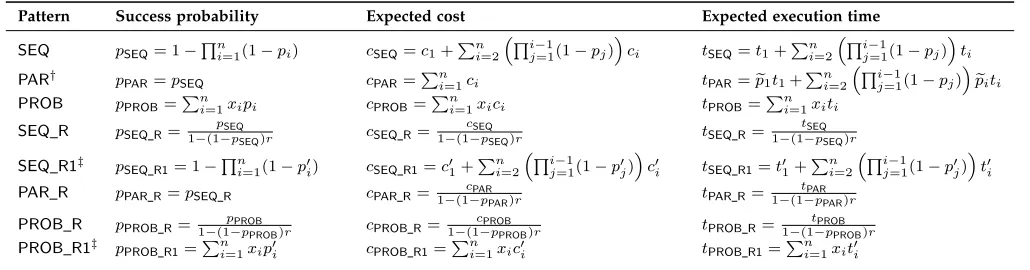
As indicated earlier in the paper, our ePMC method is well suited for the SBS domain, as the operation imple-mentation patterns from Table 4 correspond to component modelling patterns whose reliability, cost and execution time can be obtained in the first stage of the method. Table 5 and the following theorem provide the repository of (manually derived) closed-form expressions for all patterns from Table 4 and three key QoS properties of SBS operations.

Theorem 3. The closed-form expressions from Table 5

specify the success probability, the expected cost, and the expected execution time for each of the SBS-operation im-plementation patterns from Table 4.

Proof. We prove theSEQresults by induction. For the base case, we have n = 1, corresponding to an SBS operation carried out by a single service with success probabilityp1, cost c1 and execution time t1. As required, pSEQ = p1 = 1−(1−p1),cSEQ=c1andtSEQ=t1. Assume now that the SEQexpressions from Table 5 are correct fornservices, and consider anSEQpattern comprisingn+1services. There are two ways in which then+ 1services can complete the oper-ation successfully: (i) either the firstnservices complete the

operation successfully (with probability1−Qn_i=1(1−pi)), or (ii) each of the firstnservices fails, and the invocation of the(n+ 1)-th service is successful. Accordingly, the success probability for the(n+ 1)-serviceSEQpattern is:

(1−Qn_i=1(1−pi))+((Qni=1(1−pi))pn+1)= 1−Qni=1+1(1−pi).

To calculate the expected cost and execution time for the (n+ 1)-serviceSEQpattern, recall that the(n+ 1)-th service is invoked iff the invocations of all previous n services failed, i.e. with probabilityQni=1(1−pi). Accordingly, us-ing the(n+ 1)-th service adds a supplementary expected cost of(Qni=1(1−pi))cn+1 and a supplementary expected execution time of(Qni=1(1−pi))tn+1 to the expected cost and execution time of ann-serviceSEQpattern, respectively. Thus, the expected cost for the(n+ 1)-serviceSEQpattern is given by

c1+Pni=2

Qi−1

j=1(1−pj)

ci+ (Qni=1(1−pi))cn+1=

=c1+Pni=2+1

Qi−1

j=1(1−pj)

ci

and the expected execution time can be calculated similarly, which completes the induction step.

For the PAR pattern, the probability that the parallel invocations of the n (independent) services will all fail is

Qn

i=1(1−pi), so the probability that the operation will be completed successfully is1−Qn_i=1(1−pi)as required. Also, since all n services are always invoked, the cost for the pattern is given by the sum of thenservice costs. Finally, to calculate the expected execution time for thePAR pattern, assume (as stated in Table 5 and without loss of generality) that thenservices are ordered such thatt1≤t2≤ · · · ≤tn. Under this assumption, service i will be the first service that completes execution successfully(in timeti) iff: (i) the invocations of the faster services 1,2, . . . , i −1 have all failed (which happens with probabilityQi_j−₌₁1(1−pj)); and (ii) the invocation of serviceiis successful (which happens with probabilitypi). Thus, the execution time for thePAR patterns follows a discrete distribution with probability

Qi−1

j=1(1−pj)

TABLE 5

Complete ePMC repository of QoS-property expressions for the SBS domain

Pattern Success probability Expected cost Expected execution time

SEQ pSEQ= 1−

Qn

i=1(1−pi) cSEQ=c1+Pni=2

Qi−1

j=1(1−pj)

ci tSEQ=t1+Pni=2

Qi−1

j=1(1−pj)

ti

PAR† pPAR=pSEQ cPAR=

Pn

i=1ci tPAR=pe1t1+Pni=2

Qi−1

j=1(1−pj)

e piti

PROB pPROB=

Pn

i=1xipi cPROB=

Pn

i=1xici tPROB=

Pn i=1xiti

SEQ R pSEQ R=

pSEQ

1−(1−pSEQ)r cSEQ R=

cSEQ

1−(1−pSEQ)r tSEQ R=

tSEQ

1−(1−pSEQ)r

SEQ R1‡ pSEQ R1= 1−

Qn

i=1(1−p′i) cSEQ R1=c′1+

Pn i=2

Qi−1

j=1(1−p′j)

c′

i tSEQ R1=t′1+

Pn i=2

Qi−1

j=1(1−p′j)

t′

i

PAR R pPAR R=pSEQ R cPAR R=₁₋₍₁₋cPAR_p

PAR)r tPAR R=

tPAR

1−(1−pPAR)r

PROB R pPROB R=₁₋₍₁₋pPROB_p

PROB)r cPROB R=

cPROB

1−(1−pPROB)r tPROB R=

tPROB

1−(1−pPROB)r PROB R1‡ pPROB R1=Pni=1xip′i cPROB R1=Pin=1xic′i tPROB R1=Pni=1xit′i

†_{assuming that thenservices are ordered such thatt}

1≤t2≤ · · · ≤tn, withpei=pifori < nandepn= 1

‡_p′

i= p_i

1−(1−pi)ri,c

′

i= c_i

1−(1−pi)ri andt

′

i= t_i

1−(1−pi)ri for alli= 1,2, . . . , n

probabilityQn_j=1(1−pj)of unsuccessful completion in time

tn. As a result, the expected execution time for the pattern is given by:

Pn i=1

Qi−1

j=1(1−pj)

piti+Qnj=1(1−pj)

tn=p1t1+

+Pni=2−1

Qi−1

j=1(1−pj)

piti+hQnj=1−1(1−pj)

pntn+

+Qn_j=1−1(1−pj)(1−pn)tni=

=p1t1+Pni=2−1

Qi−1

j=1(1−pj)

piti+Qnj=1−1(1−pj)

tn,

which can be easily rearranged in the format from Table 5 by introducing the notationpie =pifori < nandpne = 1.

For the PROB pattern, the results from Table 5 follow immediately from the fact that the success probability, cost and execution time of the operation have a discrete distri-bution with probabilitiesx1,x2, . . . ,xnof taking the values

p1,p2, . . . ,pn(for the success probability),c1,c2, . . . ,cn(for the cost), andt!,t2, . . . ,tn (for the execution time).

For the SEQ R1 pattern, we first focus on a single serviceiwith success probability pi, costci and execution time ti. If unsuccessful invocations of the service (which happen with probability (1 −pi)) are followed by its re-invocation with probabilityri, then the overall probability of successfully invoking the service is given by:

p′

i = pi+ (1−pi)ri

pi+ (1−pi)ri pi+. . .

=

= pi+ [(1−pi)ri]pi+ [(1−pi)ri]2_{pi+. . .=} = limm→∞Pmj=0[(1−pi)ri]jpi=

= limm→∞pi1−[(1−pi)ri] m+1 1−[(1−pi)ri] =

pi

1−(1−pi)ri.

(11)

A similar reasoning can be used to show that the expected cost and execution time of the service with re-invocations are

c′i =

ci

1−(1−pi)ri and t ′ i=

ti

1−(1−pi)ri, (12)

respectively. Thus, the n-serviceSEQ R1 pattern from Ta-ble 5 is equivalent to an n-service SEQ pattern whose services have success probabilitiesp′

1,p′2, . . . , p′n, costsc′1,

c′

2, . . . ,c′n, and execution timest′1,t′2, . . . , t′n. As a result,

the expressions for the success probability, expected cost and expected execution time of the SEQ R1 pattern can

be obtained by using these parameters in the analogous expressions of theSEQpattern, as shown in Table 5.

The SEQ R pattern is equivalent to having a single service with success probability pSEQ, cost cSEQ and exe-cution timetSEQ, and re-invoking this service with proba-bilityrafter unsuccessful invocations. As such, the success probability, expected cost and expected execution time for theSEQ R pattern are obtained by applying the formulae from (11) and (12) to this equivalent service, which yields the expressions from Table 5.

Using the same reasoning as for the SEQ Rpattern, it is straightforward to show that Table 5 provides the correct expressions for thePAR RandPROB Rpatterns.

Finally, the n-servicePROB R1pattern is equivalent to an n-servicePROB pattern whosei-th service has success probabilityp′

igiven by (11), and costc′iand execution time t′

igiven by (12). Using these three formulae as parameters in

the expressions giving the success probability, expected cost and expected execution time of thePROBpattern yields the results for thePROB R1pattern.

As we show experimentally in Section 8, ePMC can use the repository of closed-form expressions from Table 5 to efficiently compute reliability, cost and response-time QoS properties of realistic SBS designs that leading model check-ers take a very long time to verify, or cannot handle at all due to out-of-memory or timeout errors. Furthermore, as also shown in Section 8, our method yields closed-form expressions that are more compact and take far less time to evaluate than the expressions produced by traditional PMC.

7

PMC

M

-T

A

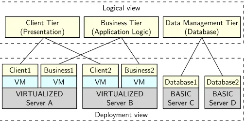
As a second application domain for ePMC, we consider the deployment of software systems with a multi-tier ar-chitecture on a set of servers. For improved reliability and throughput, these systems often use horizonal distribution