Tail probabilities and almost sure bounds for martingales

by

W.L. Steiger

A thesis presented to the Australian National University

for the degree of Doctor of Philosophy

in the

Unless reference is specifically made to other work, all the

material in this thesis is original. It is based on 5 papers

two published, one to appear, one submitted, and one in preparation. Specifically Chapter 1 is based on [18], Chapter 2 on [15],

Chapter 3 on [16], Chapter 4 on [17] and Chapter 5 on work that will

be reported in [IS].

W- {•

This thesis is dedicated to Dr L.J. Portnoy and the succubus of the Western World.

Introduction 1 Chapter 1 Bernsteins Inequality for Hartingales

1. Introduction and Summary 5

2. The Generalization 5

Chapter 2 Some Tchebycheff-Type Inequalities

1. Introduction and Summary 11

2. Results When {X.} Independent 19

3. Results for S 1 25

4. Comparison of Results 27

Chanter 3

1

1. Introduction and Summary 29

2. Bernstein's Inequality for B' 32

3. Upper Bounds in B for E(exp(kS )) 38 4. A Best-Possible Kolmogoroff-type.

Inequality for B and a Characteristic Property 42 5. A Partial Converse to Theorem 4.1 45 Chapter 4 Some Limit Properties

1. Introduction and Summary 48

2. A Criterion for 'lembership in S 50

3. Relation to the General Law of the Iterated Logarithm 56 4. A Result Without {X^} Uniformly Bounded 61

Chapter 5 A Test Against Independence 64

Appendix Table I 68

Table II 71

[image:4.549.71.497.94.631.2]

INTRODUCTION

T M s thesis contains a study of martingales. Some

well-known results of probability theory are extended to the

martingale context. Many of the extensions are best-possible in

a sense to be made precise in the relevant part of the text. One

result provides a characteristic difference between martingales

and sums of independent random variables. Extensions to

martingales of certain limit theorems for maxima of suras of

independent random variables are given; these results are in a

form stronger than those they extend. Finally, a test which

discriminates between martingales and independent sums is given.

Specifically, the material of chapters 1, 2, 3 falls within a domain of investigation which has been called Tchebycheff-type

inequalities. Such inequalities have been studied from the point

of view of determining the maximum, over a prescribed class $ of probability measures on the real line, for the integral with

respect to a measure in of the characteristic function of a

prescribed subset of the reals. Chapter 2 studies the possibilities

a special structure - the maxima of martingale sequences - where

the above mentioned subset of the reals is a set of the form

[t,»)# t > 0, and the class $ is prescribed by a variety

conditions. As such, the Tchebycheff-type inequalities which

result are analogues of the classical IColmogoroff inequality for

martingales.

In chapter 3 stronger results are obtained. In particular

one Tchebycheff-type inequality is found which is best-possible

for a class of sums of independent random variables but which

does not hold, in general, for a related class of martingales - a

characteristic difference. Another result is a best-possible

analogue of the Kolmogoroff inequality for the latter class of

martingales.

Both chapters 2 and 3 utilize the main theorem of chapter 1

which gives a generalization of the classical Bernstein

inequality to martingales. Further, it is shown that this

inequality cannot be improved. The strength of this result is

partly illustrated by its use in chanters 2 and 3. A corollary

In chapter 4 certain limit theorems for martingale sequences

are developed. Almost sure bounds for such sequences are derived

from the study of an analogue of upper class (real) sequences.

The upper class sequences have been used previously in work by other authors, for example Fellers 1943 paper in the Transactions of the American lathematical Society.

Finally, in chapter 5, a statistical test that discriminates between sums of independent random variables and martingales which

are not such sums is constructed. It utilizes the characteristic

property of martingales derived in chapter 3. An interesting

application of this test to the nature of speculative price movements is discussed.

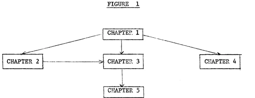
In summary, the interdependence among chapters is displayed by the following figure.

FIGURE 1

[image:7.549.74.501.516.681.2]

The following common conventions for numbering and referencing

equations and topics will be adopted. In each chapter, x^ithin

each section, the equations will be numbered sequentially, beginning

from 1. Also theorems, lemmas, corollaries, remarks, definitions,

and notations - in fact all rubrics - will be numbered sequentially,

all in the same sequence, beginning from 1. For section references,

Section x refers to section x of the present chapter: Section x.y

refers to section y of chapter x, not the present one.

For equations, (x) refers to equation x of the present

section, (x.y) to equation y of section x, not the present one,

of the present chapter, and (x.y.z) to equation z of section y

of chapter x, not the present one. The references Theorem x,

Theorem x.y, Theorem x.y.z, as well as similar references using

CHAPTER 1 ,

B e r n s t e i n s Inequality for Martingales

§ 1 Introduction and Summary.

This chapter derives a result that is basic to the remainder of

the thesis, as well as ’laving independent interest. The theorem we

will prove extends the classical Bernstein inequality to maxima of

martingale sequences and shows that this well known result holds for

sums of not necessarily independent random variables. The

generalization is best-possible in that the bound we give for tail

probabilities of maxima of martingale sequences, over a wide class

of martingales, cannot be lowered without being violated. A

corollary which further generalizes this result is also proved.

§2 The Generalization.

notation 1 ; E denotes mathematical expectation.

I+ denotes the positive integers.

Bernstein’s inequality states that for any random variable X and

(1) Pr{X>t} <_ E ( e x p (IOC))/ e x p ( k t )

Of c o u r s e (1) o n ly makes s e n s e i f t h e moment g e n e r a t i n g f u n c t i o n o f

X e x i s t s a s 1 i s a t r i v i a l u p p er bound f o r t h e r e l e v a n t p r o b a b i l i t y .

\’le s h a l l d e v e lo p an a n a lo g u e o f (1) when X h a s a s p e c i a l

s t r u c t u r e , t h e maximum o f t h e f i r s t n e l e m e n t s i n a m a r t i n g a l e ,

n £ I + f i x e d b u t a r b i t r a r y . S p e c i f i c a l l y

D e f i n i t i o n 2 . A se q u e n c e o f random v a r i a b l e s {S_^} i s a m a r t i n g a l e

i f f E(S^) = 0 and JE (S J S = S_^ ^ a lm o s t s u r e l y , i e I + ,

i > 2.

D e f i n i t i o n 3 . For n e I + d e f i n e M (n ), t h e c l a s s o f m a r t i n g a l e

t h

s e q u e n c e s whose n * members have moment g e n e r a t i n g f u n c t i o n s , by

(2) M (n) = { { S . ) : {S, } a m a r t i n g a l e and E(wxp(kS ) ) < « > }

i i n

f o r s u f f i c i e n t l y s m a l l k > 0.

D e f i n i t i o n 4 . F or n c I + and {S_^} e M (n) d e f i n e {'.! } ,

4*

M. = max S , i , j e I ,

1 j < i J

Our g e n e r a l i z a t i o n o f (1) i s g i v e n i n

Theorem 5. G iv en n

e

I + and k , t > 0,

(3) i n f [E (ex p (k S ) ) / e x p ( k t ) - P r { M > t } ] = 0

M(n) n

P r o o f : The a s s u m p ti o n s ( i n ( 2 ) ) and t h e c o n v e x i t y o f exp im p ly , by

a r e s u l t o f F e l l e r ( [ 5 ] , V o l . I I , p . 2 1 5 ) , t h a t ( e x p ( k S ^ ) } i s a s u b ­

m a r t i n g a l e so t h a t f o r i n t e g e r s i >_ j > £ >_ 1,

(4) E (ex n (kS^) |e x p (k S ^ ) , . . . ,exp(kS^ ) ) >_ E (ex p (k S ^ ) | exp(lcS^) , . . . yexpCkS^))

D e f in e t h e random v a r i a b l e L by

(5) L =

m i n ( j sl<_j<n : >_ t ) o r

0 i f S, < t , 1 < j < n

j ~

-n

C l e a r l y Pr{M > t} = £ Pr{L=i} b e c a u s e t h e e v e n t s { L=i} a r e m u t u a l l y

n _ i = l n

e x c l u s i v e f o r i = l , . . . , n and t h e e v e n t { M> t } =

I

{L=i} .

n— . ,

n

(6) E (exp(kS ) ) = £ E(exp(l-:S ) | L = i ) ( P r { L = i ) )

n i= 0 n

n

>_ £ E (exp(kS ) I L=i) (P r{ L = i} )

i = l n

n

> £ E (ex p (k S ) IL—i ) ( P r { L = i})

i = l ’ 1

> e x p ( k t ) ( P r {11 > t } )

—

nr-The f i r s t l i n e f o l l o w i n g by d e f i n i t i o n , t h e s e c o n d s i n c e exp i s non­

n e g a t i v e and k > 0, t h e t h i r d from (4) and t h e l a s t from t h e

d e f i n i t i o n o f L, and b e c a u s e exp i s n o n - d e c r e a s i n g . T-Je have

t h u s shown t h a t f o r e v e r y {S_^} e i'4(n), k , t > 0,

(7) Pr{M >t} < E (exp(kS ) ) /e x p ( l e t)

n— — n

To p ro v e (3) we need o n l y show t h a t f o r ea c h £ > 0 t h e r e i s

(Sj,) e M(n) f o r w hich P r i H ^ t } + £ > E (e x p (k S n ) ) / e x p ( k t ) ; i . e . t h a t

t h e infimum i n (3) i s z e r o .

G iven £ > 0 c h o o s e <5, 0 < 6 < m i n ( £ , exp ( - k t ) ) . C o n s id e r t h e

f u n c t i o n s f , g on [ 0 , 1 ) d e f i n e d by f : x k t / ( l - x ) and

h : x f(x)-g(x) is negative at x = 0. Since f is increasing and g decreasing on [0,1), h is increasing. Finally, as

f(x) -* as x -* 1 and g(x )-*■-«> as x 1, the intermediate value theorem applied to h shows that there exists a unique Xq z [0,1) for which h(x^) = 0; i.e. a unique x^ such that

l og((1-Xq)/6 ) = kt/(l-x^). From this it follows that at x^

(8) 6 = (l-x0)exp(-kt/(l-x0))

Define the random variable X by Pr{X=t) = x^ = l-Pr{X=~-XQt/(l-x^)} . Clearly E(X) = 0 and

(9) E(exp(kX)) = (l-x0 )exp(-ktxQ /(l-x0 ))+x0exp(kt)

= [x0+(l-xQ )exp[-kt(l+xQ /(l-x0))]]exp(kt)

= [x0+(l-x0 )exp[-kt/(l-x0 )j ] exp (let)

= [xQ-h5]exp(kt)

(10) Pr{X>t} = x Q

= E(exp(kX))/exp(kt) - 6

> E(exp(kX))/exp(kt) - £

by definition of X, (9), and choice of 6, respectively. The fact that the sequence {S^}, S_^ = 0 almost surely, i = l,...,n-l and S_j, = X almost surely, i >_ n, i s I+ , is in iH (n) completes the proof.

As the proof of Theorem 5 only used the convexity of exp (in (4)), and the facts that exp is both non-negative and non-decreasing,

the following corollary is proved in precisely the same fashion.

Corollary 6 . Let h > 0 be a non-decreasing, convex function and take n e I+ , k,t > 0. Then.

(11) inf [E(h(kS ))/h(kt)-Pr{I! >t}] = 0

M '(n) n

CHAPTER 2 .

Some Tchebycheff-type Inequalities

§1 INTRODUCTION M D SUMMARY.

In this chapter inequalities which bound the tail probabilities

for maxima of partial sums of almost surely bounded random variables

are given. The results are analogous to the classical Kolmogoroff

inequality (cf. Feller [5], Vol. I).

As the Kolmogoroff inequality extends Tchebycheff's inequality,

these results extend work of Dennett [1], [2] and Hoeffding [9].

The generalizations lie in two directions. First, maxima of

partial sums, rather than sums themselves, are considered. Second,

for some of the results, the summands need not necessarily be

independent.

The domain of this investigation is what has been called

Tchebycheff inequalities (cf. Godwin [7] and [8] and Karlin and

Studden [10]). Generally, the problem is as follows. Let 0

denote some class of probability measures on the line, T a subset

f

T :

<P

f d(P°

T

We are interested in numbers A :B ? 0 <_ A,B <_ 1, such that

(1) max f = A, min fr., = B.

$ $ 1

In this case the double inequality

(2) B <_ fT (cf>) <_ A,

<p

e $

holds and is called a sharp Tchebycheff-type inequality. Each side of (2) is attained by some measure in

If t;e can only find numbers A,B, 0 <_ A,B <_ 1, such that

(3) sup f = A, inf fT = B

$ $

As an exam ple su p p o se numbers t , v , t >_ v > 0 a r e g i v e n .

00

Take T = C-00, 00) ^ ( - t , t ) and $ = {<j) :

J

|x|d<j>(x) = v}, th e s e t

—00

o f p r o b a b i l i t y m ea su r e s on th e l i n e w it h f i r s t a b s o l u t e moment v .

For any <j> e $ i t i s e a s y t o s e e

- t »

(4 ) f T (4>) = / dc{) (x ) 4- J d<}> (x )

—00 t

<_ / d<J> (x ) + /

-L—

L

dc|) (x )

-o° t

< v / t .

F u r t h e r , i f ^ i s a to m ic w it h atom s a t t and 0 su ch t h a t

q( t ) = v / t , <}>q( 0 ) = 1 - v / t , th e n <J>^ e $ and c l e a r l y

f T n ) = T h is rem ark and (4 ) show t h a t

(5 ) max f = v / t

$

and th u s t h a t th e i n e q u a l i t y

(6 ) f T(<f>) ^ v / t , cf> e $

t h e m ost b a s i c and c l a s s i c a l T c h e b y c h e f f - t y p e i n e q u a l i t y .

To p r o d u c e new T c h e b y c h e f f - t y p e i n e q u a l i t i e s , r e s t r i c t i o n s on

t h e c l a s s $ a r e f r e q u e n t l y im posed. T y p i c a l l y t h e s e i n v o l v e

( a ) , moment c o n d i t i o n s , ( b ) , some sm o o th n ess c o n d i t i o n s , o r

( c ) , g e o m e tr ic c o n d i t i o n s . Examples o f t h e s e k i n d s o f r e s t r i c t i o n s ,

r e s p e c t i v e l y , a r e :

t h e s e t o f m e a s u r e s f o r w h ich d e n s i t i e s e x i s t and a r e n ti m e s

d i f f e r e n t i a b l e . 00

( a ) $ = {(f) ;

f x^

d<J)(x) = c ^ , 1 < i < n}

t h e s e t o f m e a s u r e s whose f i r s t n moments a r e p r e s c r i b e d .

y

(b) $ = {({>: / d(j> (x) i s an n + 1 t i m e s d i f f e r e n t i a b l e f u n c t i o n o f y}

y

(c) $ = (4> : 3 y^ e (~C0,00) f o r w hich

J

d<j> (x) i s

co n v ex , y < y

c o n c a v e , y >_ y

Use of (a) is made in many scattered results (but see [11],

Chapters 12 - 14, for a synthesis based on ideas in [10]). Use

of (b) is, for example, made in [13] through a novel type of

condition and in [8], results using (c) are given.

In this chapter, and throughout the thesis, we shall be dealing with random variables which are themselves sums of random variables. For this reason it is notationally convenient to specify $ as a class of random variables rather than as a class of probability measures on an n-fold cartesian product of the reals, for some n. The framework for this is supplied below where some of the terminology and notation used in this thesis is set out.

Notation 1 . V denotes variance.

E(«|°) denotes conditional expectation.

V(°I 0) denotes conditional variance.

{X^} denotes a sequence of random variables.

denotes V(X^), i e I+ .

c^ denotes V(X^).

Definition 2 . Given {X.} define

(i) { , S_. = + ... + X^, i e I*", the sequence of partial

sums.

+

(ii) {M.}, M. = max S ,

.1

si e I , the sequence of maxima. 1 1 j<i 3

(iii) {s|}9 = ^(S^), i e I , the variance of partial sums

(iv) {C2}, = V(S1), C| = V(Si |Si_1 ,...,S1) ; i e I+ , i >_ 2

the conditional variances of partial sums.

Definition 3 .

{X^}

is absolutely fair iff

E(X^) = 9,

F ( X . IXf i ,. •. jXf) = 0 , i e I+ , i >_ 2.

For convenience we repeat

Definition 4 . {S^} is a martingale iff S(S^) = 0,

I +

E(S I S = S. almost surely, i e I , i _> 2.

every martingale arises in this way; i.e., if {T^,} is a martingale,

3 an absolutely fair sequence, {Y_, } s such that

T i = Y 1 + " • + Y i» i e I+ (cf. Feller [5], Vol.II ).

Definition 6* Given {X.}, X. is unimodal, some i e I 9 iff

. — --- --- 1 i ,, — — —■■

l x , such that Pr{X. < x} is convex for x < x. and concave for

~ l l — l

X > X . .

— 1

Analogous to $ in the previous discussion we shall, in this chapter, consider the class 8, of sums of random variables, defined below.

Definition 7 . Define the class B of martingales whose summands are almost surely bounded by

8 = {{S±> : = X^ + ... + X^, i e I+ 9 {X_j} absolutely fair,

and 3 > 0 % |X^| <_ almost surely, i e I.+ } .

Definition 8 . Let t > 0 and n e I+ be given. ^ function from B into the interval [0,1] defined by

g : {S,} -* Pr{M > ts2} .

n,t i n — n

Remark 9. g

----

n,t

in Definition 8,

is well defined. By the boundedness of

s2 exists for all n e I+ . n

{X.}

In the present context, analogous to (1) and (3), we seek

a function h from

B

to the closed interval [0,1] such that n,t

(7) min

B

[h -g ]

nj t n, t = 0 .

In view of Definition 8 the Tchebycheff-type inequality

(Ö)

j ({S .} ) < h

n,t l — n,t ({S.})

would be an analogue of Kolmogoroff’s inequality and would be sharp.

If, in (7) only the infimum over 8 is zero, (8) would be

best-possible. This chapter is devoted to a study of such results.

In Section 2 Theorem 1.2.5» is specialized to yield a

best-possible bound for g . over 8. Then we consider subclasses of n , t

8 where {X^} are independent and, in addition, various geometric

conditions on {X } are imposed. The possibilities for improving

^ are studied under these restrictions on 3. The inequality

8 «.({S.}) < h ({S .}), for all {S.} e 8, Is investigated in

Section 3 and numeric bounds for the tail probabilities of maxima of martingale sequences are obtained. Finally, in Section 4, these bounds, and some of the results of Sections 2, are compared with connate Tchebycheff-type inequalities which are already known.

§2. results TThen {X^} are Independent.

For any n e I+ , 8C',!(n), (Definition 1.2.3.), because, by the boundedness assumption in Definiton 1.7, E(exp(kSn )) exists for all k > 0, and all { } e 3. For the same reason, V(S ) exists whenever {S.} e 7>. Denote by h _ the function from 3 to the

x J n ;t

reals defined by

(1) h n t : ( S j -> E(exp(kS_))/exp(kts2 )

h is well defined by the above remarks. Replace t by us2 in

n,t y „ j n

(1.2.3) to °rive

Lemma 1. For n e I , k,u > 0,

This strengthens Lemma 1 in [15] because by (2), the right-hand side of the inequality

(3) Pr{M > us2 } < E(exp(kS ))/exn(kus2 )

n — n — n ‘ n

may not be lowered and still hold in 8.

In the remainder of this section we shall consider (3) over various subclasses of 8, attempting to bound the right-hand side. The results extend work of Bennett, [1], and [2], to the maxima of sequences of sums of independent random variables.

Definition 2 . Define the class

Z

8, of sums of independent, almost surely bounded random variables by

I

= { { S j 8 8 : independent}

By the independence of {X_^} 3 for each n e I+ ,

n n

(4) E(exp(kS )) = E(exp(k £ X )) = II E(exp(kX ))

n i=i 1 i=l 1

|X I <_ almost surely, i e I+ , to bound the right-hand side

of (3),

Theorem 3. For n e I+ , k,u > 0 and each {S.} e I s

n kB

(5) E(exp (kS )) <_ II (l+(e X-kB -l)a?/B2)

n l l i

“f“ ^QC n

Proof: Fix i e I . e‘ 1 + kx 4- ax2 for all

x e [-B^,B_^] if and only if

(6) (e^-kx-l) /x2 <_ a

The left hand side of (6) is monotone increasing in x so that for all x e [-B ,B ]

kx kBi

(7) e < 1 + kx + (e -kB,-l)x2/B2

— i i

Replacing x in (7) by and taking expectations, gives

kB

(8) E(exp (kX.)) < (1+e -kB -l)o2./B2

i — i l l

B.emark 4 . From (5) and (3) f o l l o w s , f o r n e I , u 9lc > 0

n kB k u s 2

(9) Pr{M > u s 2 } < [ n ( l + ( e 1- k 3 . - l ) a 2 / B ? ) ] / e n

n— n — . -j l 7 . 3 .

1=1

f o r eac h {S^} e

I.

F u r t h e r , t h e p r e c e d i n g p r o o f h o ld s i f we r e p l a c e

each B. by B = max B. . By t h e a r i t h m e t i c - g e o m e t r i c mean i n e q u a l i t y

1 i< n 1

(9) th e n becomes.

(10) Pr{M > u s2 } < [ l + ( e ^ - k B - l ) s 2 / ( n 3 2 ) ] n / e n

n— n — n

w here s 2 = a 2 + . . . + a 2 s i n c e {S.} e I .

n 1 n l

The n e x t r e s u l t shows t h e r o l e o f t h e number k i n t h e p r e v i o u s

d i s c u s s i o n .

Theorem 5 . For n e I , u > 0 and any { S_^} e I ,

s 2 u/B s 2 /B2

(11) Pr{M > u s 2 } < ( e / ( l + u B ) ) ( l / ( T f u B ) )

n— n —

P r o o f : Use 1 -f t <_ e*", t >_ 0 , i n t h e r i g h t - h a n d s i d e o f (10) and

m in im iz e t h e r e s u l t i n g i n e q u a l i t y w i t h r e s p e c t t o k*; t h e

independently by Bennett [1] and Hoeffding [9] as a bound for

Pr{S >us2 }, but not shown to be best-possible, rr— n

The remainder of this section investigates possible improvements

in (5), (10) and (11) in case, in addition to {S } e I , we assume

{X_.} are symmetrically distributed. Accordingly we can generalize

work of Bennett [2] as follows.

4

-Theorem 7 . For n e I', k,u > 0 and {S^.} e I such that

{X^} are symmetrically distributed,

______ ____ us2 /B2

(12) Pr{M >us2 } < exp[ ( (/l+u2B2 )-l)s2 /B2?/( uB+/l+u2B2 ) n

n— n — n

Proof: By the symmetry assumption, analogous to (A) we have, since

cosh is an even function,

n

(13) E(exp(kS ) ) = IT E(cosh(kX.)) .

n . . i

i=l

For i £ I+ , cosh(lcx) <_ 1 + ax^ for all x e

if and only if (cosh(kx)-1) /x2 <_ a and, as the left-hand side is

( 1 4 ) c o s h ( k x ) <_ 1 + ( c o s h ( k 3 ) - ' l ) x 2 /B 2

f

-f o r a l l x e [-B ,B ] . For each i e I , i <_ n , p u t i n

( 1 4 ) , t a k e e x p e c t a t i o n s , u s e t h e r e s u l t s i n ( 1 3 ) , and t h e n d . s e (13)

i n (3) t o o b t a i n , f o r e a c h r e l e v a n t {S } e I

n k u s 2

(15) Pr{M >us2 } < [ II ( l+ ( c o s h ( k B ) - l ) a 2 / 3 2 ) ] / e

n— n — . •) i l l

i = l

w hich i s a n a lo g o u s t o ( 5 ) . R e p la c e each. Ph, i = l , . . . , n , by

B = max B. i n (15) and a p p l y t h e a r i t h m e t i c - g e o m e t r i c mean i n e q u a l i t y

i< n 1

t o s e e

(1 6 ) ?r{M > u s 2 } <

n— n —

k u s 2 [ 1 + ( c o s h (kB)- 1 ) s 2 / (nB2 ) ] n / e

n

a n a lo g o u s to ( 1 0 ) . F i n a l l y , as w i t h ( 1 1 ) , (12) f o l l o w s

p

from u s i n g 1 + t <_ e , i n (16) and t h e n m in im iz in g t h e r i g h t - h a n d

s i d e w i t h r e s p e c t to k ; t h e minimum o c c u r s when s in h ( k B ) = uB.

Remark 3 . I f we make t h e f u r t h e r r e s t r i c t i o n t h a t {X } a r e u n im o d a lly

d i s t r i b u t e d t h e n V(X^) <_ B2 / 3 , i e I + , a s t h e r e c t a n g u l a r

d i s t r i b u t i o n i s t h e u n im o d al d i s t r i b u t i o n on [ - B ^ , 2 . ] o f g r e a t e s t

§ 3 Results for ß.

Without using independence, (2.4) no longer holds. The approach

used to bound E(exp(kSn )) in Section 2 gives a result analogous to

Theorem 2.5 but considerably weaker. Specifically

JL

Theorem 1 : For n e I ', k,t > 0 and { S_^} e 8,

ts2 / (nB) s2 /(n2 ß2)

(1) P r { M > t s 2 } < [e/(l+tnB)] n [ 1 / (1-i-tnB) ] n r>— n —

Proofs From Definition 1.7 it is clear that | S | <_ nB almost surely,

|/v

E = max B.. Hence, as e <_ 1 + kx + (e v -knB-l)x2 / (nB)2 9 x e [- n B ,n B ] i<_n 1

replacing x by S^ and taking expectations gives

(2) a (exp (kS )) < 1 + (e‘n~-knB-l) s2 / (n2 B2 )

n — n

Using (2) in (2.3), the fact that 1 + u < e11, and then

minimizing the right-hand side of the resulting expression with

respect to k yields the asserted result.

Remark 2 In the next chanter (1) will be substantially improved by

showing that something like Theorem 2.3 holds for members of 8 instead

Finally we give a result bounding the tail probabilities for the maxima of moduli of martingale sequences.

Theorem 3 Under the assumptions of Theorem 1 9

(u2s2-l)s2/(n2B2) s2/(n2B2) (3) Prfmax

|s.|

>_ us2} <_(e/(u2s2)) n n (l/(u2s2)) n

l<i<n 1 n n n

+

Proof" Fix n e I and take {S .} e B. For t > 0 define the

--- l

random variable K(t) by

(4) K(t) =

min(j,l<j<n : | | ^ t) or

0 I S . I < t , 1 < j < n

3 - ~

n

Clearly Pr{max Is.l > ts2} = V Pr{K(ts2 ) = i}.

i — n u n

l<i<n i=l

Because {S_^} is a martingale, the function p : x -*■ x2 convexs

r\ «I»

and E(S^) exists by the boundedness assumption for all i e I , a

result of Feller ([5], Vol.II, p.215) shows that {S2} is a sub-martingale. For the same reasons so is {exD(S2 )}. The arguments leading to (1.2.3) then show

(

5)

Pr(max | S . | 1< i< n

> ts2 } < E(exp(kS2 ))/exp(kt2 s4 )

Bounding E(exo(kS2)) by 1 + (ev‘ -l)s2/(n2B2) as in previous

n n

arguments, using 1 + t £ e*1, and (5) yields, after minimizing the resulting expression with respect to k, the inequality in (3).

Remark 4 . (2.9), (2.10), (2.11), (2.12) and (1) are comparable with (3). The arguments x^hich establish an inequality of the

form Pr{Mn >_ ts2} <_ f(t), when applied to martingales with summands {-X.} give Pr{max (-S.) >_ ts2} f(t). Hence, by

1 l<i<n 1 n

doubling the bounds of (2.9), (2.10), (2.11), (2.12) and (1), we obtain inequalities for the maxima of the moduli of martingale

sequences.

§ 4 Comparison of Results

In this section some of the inequalities of Sections 2 and 3 are compared with known results. First, any analogue of

Kolmogoroff?s inequality for martingales must be compared with the following strong result.

(1) rain [l/(l+t2s2) - gn t ( { ) ] = 0

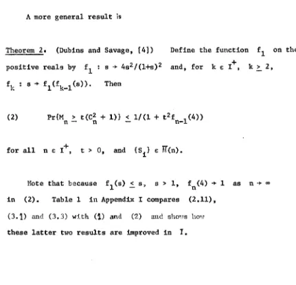
A more general result is

Theorem 2« (Dubins and Savage, [4])

positive reals by : s -> 4s2/(l+s)2

fk : s + fx(~k—1 (s))• Then

(2) Pr{M > t(C2 + 1)} < 1/(1 + t2f .(4))

n — n — n-l

for all n e I+ 9 t > 0, and {S.^} e ?T(n).

Note that because f^(s) _< s, s > 1, f^(4) T as n - + »

in (2). Table 1 in Appendix I compares (2.11),

(3.1) and (3.3) with (1) and (2) and shows how

these latter two results are improved in I.

Define the function f^ on the

[image:32.549.78.509.156.571.2]

CHAPTER III

§ 1 Introduction and Summary.

In the previous chapter the class G of martingale sequences was

considered, and Tchebycheff-type inequalities for B were developped.

Further, under the assumption of independence of summands, stronger

results for the class

l CI B

were obtained as well as even better

results for subclasses of I.

Here, continuing the inquiry, several important new features

concerning the nature of Sn t » tail probabilities for maxima of

members of 8, emerge. Fi*rst, one of the results previously derived

for I is shown to be best-possible. In addition this result is

extended to a class of martingales containing I , but still contained

in C, in which conditional variances satisfy a certain property.

Moreover the result is best-possible in the class. Tut the salient

fact is that it does not hold, in general, throughout 8 and thus

elucidates an important, characteristic difference between martingales

To explicate these results, we shall be dealing with classes of martingales obeying combinations of the following assumptions.

(Al) {S } a martingale.

(A2) S. = + ... + X^ and J > 0 : |xj <_ B^, almost surely,

i e I+ .

(A3) V ( X p ?i 0, V(X. |Xi_1 ,...,X1) ?£ 0, i > 2, i e I+ .

Specifically for n e let

(1) M (n) = {{S.} : (Al) holds and V(S ) < »}

l n

(2) M (n) = {{S.} : (Al) holds and E(exp(kS^)) < 00

for k > 0 sufficiently small

(3) B = {{S±> : (AI), (A2) hold}

(4) B 1 = {{S±> : (Al) - (A3) hold).

(5) H n ) = {{S± } : (Al) - (A3) hold and V(Sn) = V ( S j X n ±

(6) I = {{S . } s (AI), (A2) hold and {X^} independent)

(7)

v

= {{S.} : (A.1) - (A3) hold and {X_^} independent}

M(n), M( n ) , B, and I were considered in chapter l,The name

M(n) is pneumonic for martingale as is M (n) : 8 is a pneumonic for

v a r i a n c e equals c o n d i t i o n a l v a r i a n c e ; I and I ’ are p n e u m o n i c s for

i n d e p e n d e n t sums. It is cl e a r that for n e I+ ,

M ( n ) D M ( n ) 3 B P B ' 3 l / ( n ) 3 r and that M ( n ) D B D l .

B a nd 8* as w e l l as I and 1 1 d i f f e r o n l y t h r o u g h (A3) w h i c h

is a n o n - t r i v i a l i t y a s s u m p t i o n a s s u r i n g that at o m i c r a n d o m v a r i a b l e s

w i t h m a s s 1 at the o r i g i n c annot b e m e m b e r s of a b s o l u t e l y fair

s e q u e n c e s g i v i n g r i s e to the m a r t i n g a l e s u n d e r c o n s i d eration.

F r o m the p r o o f of T h e o r e m 1.2.5 it is o b v i o u s that

g ({S.}) <_ E ( e x p ( k S ))/exp(kt) for all n e I+ , k,t > 0, and

n j l i xi

{S^} s B 5 s i n c e 8 ; C. 8 CI M (n) . H o w e v e r the se c o n d p art of the p r o o f ,

wh e r e , for & > 0, a m a r t i n g a l e in 8 ^ 8 ' is c o n s t r u c t e d for w h i c h

g ({S } )+£ > E ( e x p ( k S ) ) / exp(kt), does not o b v i o u s l y extend to 8'.

n 31 x n

B e c a u s e w e n e e d it in w h a t follows, w e sh a l l s h o w in S e c t i o n 2 that

T h e o r e m 1.2.5 does i n d e e d h o l d w h e n r e s t r i c t e d to 8* CL 8.

inf [q

I

R e c a l l that Ben n e t t

((S }) - P r { S >

n 5t l n —

[1] and H o e f f d i n g

ts2 }] > 0 w h e r e

n —

[9] sho w e d that

ts2 /B s2/B2

q . : (S } •> (e/(l+tB)) n (l/(l+tB)) n ( R emark 2.2.6) w h i l e

j L x

T h e o r e m 2.2.5 sh o w e d that inf[q ({S }) - g ({S })] > 0. To

■r n, t i n ,t i

lim inf [q ({S .}) - g ({S })] = 0; i.e. that the inequality

n+~ l/(n) 1 n ’ 1

g <_ q holds throughout the larger class 1/ (n) and i s , in a n, t n 51

limiting sense3 best-possible there. In addition it is shown that g < q can fail in B 1 3 l/(n). Loosely speaking, this means

n , t — n , t

that the maxima of martingale sequences may have larger tail probabilities

than those of sums of independent random variables or of members

of t'(n) - a characteristic property.

In Section 3 we prove a result, analogous to Theorem 2.2.3, which

is a best possible bound in B for E(exp(kSn )). The

results of Sections 2 and 3 are combined in Section 4 to obtain

Theorem 4.1, a best-possible upper bound in 8’ for

Pr{M > tC2 } which, when restricted to ^(n) gives g ^ < q .

also, best-possible. Further, a comparison of these results with

those of Marshall [14], Dubins and Savage [4], and Theorem 2.3.1 is

made. Finally, in Section 5, a partial converse to Theorem 4.1, of

independent interest, is given.

§ 2 Bernsteins Inequality for 8*.

In this section Theorem 1.2.5 is shown to hold for

It is clear from the proof of this theorem that as ßv_M ( n ) , n e I , the inequality

(1)

Pr{M > t} < E(exr>(kS ))/exp(kt)

n — — n

-f

holds for all n £ I , k,t > 0, and {S^} £

ß.

Further the

proof reveals that for any

£

> 0, n £ I+ , 'and k,t > 0, there is a martingale {S^} £ S for which

Pr{H > t} +

£

E(exT>(kS ))/exp(kt), and, together with (1),

n — " n

that

(2) inf [E(exp(kS ))/exp(kt) - Pr{H > t}] = 0

n n

-i.e. Theorem 1.2.5 holds when restricted to 3.

Although (1) holds for all {S^} £ because 3 fC Z 3 s it is not apparent that the infimum, over

S'

, of the expression in

square brackets in (2) is zero. That this is indeed the case is the purpose of the following, predicated on an extension of the idea

Theorem 1 . F o r n £ I and k , t > 0

( 3 ) i n f [ E ( e x p ( k S ) ) / e x p (let) - Pr{M > t } ] = 0

S'

n

n “

P r o o f : The i n e q u a l i t y i m p l i e d by ( 3 ) ,

(4 ) Pr{M > t } < 2 ( e x p ( k S ) ) / e x p ( k t )

n — — n

c l e a r l y h o l d s t h r o u g h o u t J3f , f o r e a c h n e I + and k , t > 0 ,

b e c a u s e o f Theorem 1 . 2 . 5 and t h e f a c t t h a t

B '£2

M ( n ) . I t

r e m a i n s t o show t h a t t h e in fim u m o f t h e r e l e v a n t e x p r e s s i o n i s z e r o .

L e t n e I + , k , t , 5 > 0 be g i v e n . C hoose 6 > 0 s u c h t h a t

6 < m i n ( 6 , e x p ( - k t ) ) . C o n s i d e r t h e c o n t i n u o u s f u n c t i o n s f , g , h on

[ 0 , 1 ) d e f i n e d by f : x -*■ k t / ( h ( l ~ x ) ) , g : x -* l o g ( ( l - x ) / ( ( x n+ 6 ) ^ n - x ) )

a n d h : x -*• f ( x ) - g ( x ) . By t h e c h o i c e o f 6 , l c t / n < ( l o g ( 1 / 6 ) ) / n

o r , h ( 0 ) < 0 . S i n c e f 00 a s x -► 1 and g -«> a s x -* 1 ,

h 00 a s x -> 1. C o n s e q u e n t l y 3 x ^ e [ 0 , 1 ) : h ( x ) = 0 by t h e

i n t e r m e d i a t e v a l u e t h e o r e m .

F i n a l l y , b e c a u s e f i s i n c r e a s i n g and g d e c r e a s i n g on

unique, for which kt/(n(l-xQ)) = log((l-xQ)/((Xq+S)1^11-«,J) or, equivalently, for which

(5) xQ + (l-x^)exp (-let/ (n(l-x^)) ) = (Xq+6)1^11

For i e I+ define the random variable by

(6) Pr{Xi = t/n} = Xq = 1 - PrfX^ = -tx^/(n(l-x^))}

and suppose {X_^} are independent. For the given k > 0,

i e I+ ,

and

(7) E(e i) = x Q exp(kt/n) + (l-xQ)exp(-kt xQ/(n(l-x0)))

Define {S.} such that S . = X, +... + X . , i e I

l l 1 i ’

It is clear that (S.) e o'. Moreover,

l ’

(

3

)

E(exp(kS )) = II E(exp(kX.))

n i=l 1

[xn exp(kt/n) + (l-xn)exp(-kt xn /(n(l-xn)))]

[exp(kt)][xQ + (l-x0>exp(-kt/(n(l-x0)))]

the first line following by definition, the second by (7), and

the last by (5). Therefore, for the martingale just constructed,

(9) Pr{M > t> =

n — u

= E (exp (kS^)) /exp (let) - 6

> E(exp(kS ))/exp (let) - is n

the first line following from the definition of {X_^} the second from

(8) and the last by the choice of 6, which completes the proof.

Remark 2 . The martingale constructed above would also serve in the

second part of the proof of Theorem 1.2.5. However the less

elaborate one actually used seemed more natural in that context.

In the same way that Corollary 1.2.6 followed from the proof of

Theorem 1.2.5, we now have as well

Corollary 3 . Let h >_ 0 be a non-decreasing, convex function and take

(10) inf [E(h(kS ))/h(kt) - Pr{Il > t}] = 0.

S ’ n n “

A more useful consequence of Theorem 1 is the following.

Corollary 4 . Let n

e

I+ , u,k > 0, and {S^} e B ? be given and suppose b > 0 is chosen such that C2 = V ( S

I s

S,) > b

n n 1 n-1 1 — almost surely. Then

(11) Pr{Mn >_ tC^} E(exp(lcSn ))/exp(ktb)

and (11) is best-possible when b = sup(x > 0 : C2 >_ x almost surely)

Proof: {S^} e B ’ implies that (A3) holds so the existence of b > 0 satisfying C2 >_ b almost surely, is guaranteed. Putting t = ub in (4) shows that

(12) Pr{M > ub} < E(exp(kS ))/exp(kub).

n — — n

and (11) then follows since Pr{i! > uC2 } < Pr{M > u b}. n — n — n —

§3 Upper Bounds i n 3 f o r E ( e x p ( k S ^ ) ) .

Theorem 2 . 3 . 1 p r o v i d e s an u p p e r bound f o r Pr{M > t s 2 } i n

n — n

3. I t e x t e n d s Theorem 2 . 2 . 5 , t h e an a lo g o u s r e s u l t f o r

I.

The

f o rm e r i s c o n s i d e r a b l y w eak er b e c a u s e , th r o u g h t h e methods u sed i n

c h a p t e r 2 , i t was n o t p o s s i b l e t o e f f e c t i v e l y bound E(exp(lcS^))

i n 73 w h ereas f o r

I ,

Theorem 2 . 2 . 3 i s j u s t su ch a bound.

I n t h i s s e c t i o n we show t h a t a bound f o r E (e x p (k S n ) ) , s i m i l a r

t o t h e one d e v e lo p p e d i n Theorem 2 . 2 . 3 , h o l d s t h r o u g h o u t B and i s

i n f a c t b e s t - p o s s i b l e t h e r e .

S p e c i f i c a l l y , f o r n e I + and {S.} e 8 p u t 3 = max 3.

1 l c i c n 1

and t a k e d . , 0 < d. < B, su ch t h a t

x —

v ( x 1 | x i _ 1 , . . . x 1) = c^ <_ d2 , i >_ 2 , i s I + , a lm o s t s u r e l y and

V ( x p = <_ d* a lm o s t s u r e l y . By (A2) c? < E

l — alm o s t s u r e l y

t h e e x i s t e n c e of d2 i s t h u s g u a r a n t e e d , i e I + . Then

a n a lo g o u s to ( 2 . 2 . 5 )

For n e I+ k > 0 , and {S .} e o ,

l *

T’R

(1) E(exp(kS )) <. n [1 + (e -kB-l)d2/B2]

n i=l 1

Proof: e^* <_ 1 + lac + ax2 for all x e [ —B ,B ] if and only if

(2) (e ^ - kx - l)/x2 _< a

As the left-hand side of (2) is monotone increasing

kB

(3)

ei_X < 1 + kx

Jr

(e

-

kB

- 1)

x

2/B2

for all x e Replace x by in (3) and take expectations to prove the statement in (1) for n = 1. To advance the induction suppose (1) is true for n = m. Then

(4) E(exp(kSm+1)> = / E(exp(kSm+1)ISm = a)dPr{Sm £ a }

— 00

mB

- / E(exp

(k(X in+S

))|S = a)dPr{

S

< a}

t, m+1 m 1 m m —

-mB mB ,

= j e iaE(exp (kX ) | - a)dPr{S^ <_ a}

-mB

*

*

m

the first line following by definition, the second since

R e p l a c e x by X i n (3) and t a k e c o n d i t i o n a l e x p e c t a t i o n s w i t h

r e s p e c t t o t h e e v e n t {S = a} t o s e e

in

1,-n

( 5 ) E (e x p (k X m+1) | S m = a ) = E ( ( l + + (e - k B - D X ^ / B ^ ) | Sm = a )

= 1 + ( e kB- k B - l ) c 2 , . / B 2 m+1

t h e s e c o n d l i n e f o l l o w i n g from E(kX ,_ j S = a ) = 0 , t r u e b e c a u s e

m+1 m

{S } s 8 . As c 2 < d 2 a l m o s t s u r e l y ( 4 ) , i n c o n j u n c t i o n w i t h ( 5 ) ,

i m p l i e s

kR o o

(6 ) E(exp(lcS , . ) ) < [1 + ( e - k B - l ) d ? / B 2 ] / e d P r{ S < a}

m+1 — l J _ m —

-mB

fro m whic^-j u s i n g t h e i n d u c t i o n h y p o t h e s i s , t h e t r u t h o f (1 )

f o r n = m + 1 i s a p p a r e n t .

Remark 2 . (1) and t h e a r i t h m e t i c - g e o m e t r i c m ean i n e q u a l i t y im p ly

t h a t f o r n s I + , E ( e x p ( k S ^ ) ) i s no m ore t h a n

[1 + ( e ‘'’B- k B - l ) d 2 / ( n B 2 ) ] n w h e r e we h a v e w r i t t e n d 2 f o r d2 + . . . + d 2 .

i n

U -f*

S i n c e 1 + u <_ e we o b t a i n , f o r n e I , k > 0 and {S_^} e 8 .

E ( e x p ( k S n ) ) <_ e x p ( ( e ^ B- l c B - l ) d 2 /B2 )

Remark 3. (1) is best-possible in the following sense. There is no function w on I+ such that for each £ > 0 and all n

(8) E(exp(kS )) _< w(n) + £ <_ J[ [1 + (e -kB-l)d2/B2 ].

n i=l 1

That is: for all k > 0

(9) lim inf [ n [1 + (e ^'J-kB-l)d2/B2 ] - E(exp(kS ))] = 0

n-*°° ß i=l n

as the following example shows

+

Choose numbers B > d > 0 and n e I . For i = l,...,n

define the random variable X_^ by

(10) Pr{X± = B} = d2 /(d2+nB2) = 1 - Pr{X = -d2 /(nB)>

and suppose {X^} are independent. Clearly | X_J B, E(X^)

and V(X^) - d2 /n, i = l,...,n so that {S^} e S,

S± = + ... + X ^ . Since {X^} are independent,

(11) E(exp(kS ) = II E(exn(kX,))

n . , i

i = l

the first term in square brackets converges to exp(-d2 /B2 ) and

lcB

the second to exp(ev d2 /B2 ), as n «>. Therefore

k S V

-E(e n ) •> exp((e vD-kB-l)d2 /B2) from which, in view of (7) and

Remark 2, (9) follows.

Remark 4 . In fact the preceding example shows that (2.2.5) is

best-possible as {S^}, constructed above, is in 7. Furthermore,

(2.2.11) is now seen to be best-possible, as promised in Remark 2.2.6,

since it is obtained from (2.2.3) by using (2.2.5).

§ 4 A Best-Possible Kolmogoroff-type Inequality for 8 and a

Characteristic Property.

In this section we give a best-possible upper bound in B'

for Pr(M^ >_ tC^}. Restricting it to the class V (n) d B 1

reveals that Theorem 2.2.5, a statement concerning

I,

actually holds in

the larger class 1/(n) and is best-possible there. Further, the

restriction no longer holds in S ? which elucidates a characteristic

difference between the two classes.

Theorem 1»

If {S .} £ 8’, b,d > 0 and d2 > C2 > b2 almost surely,

then for t > 0, n

e

I+

(1)

Pr{M

> tC2} < etb?B[d2/(d2+tbB)](tlB+d2)/ß2

n —

n —

Proof: This follows directly from (2.11) and then (3.7),

minimizing the right-hand side of the resulting inequality with

respect to k > 0; the minimum occurs when k = (log(1+tbB/d2))/B.

Remark 2.

The right hand side of (1) decreases as b increases

and hence, when b = sup (x > 0 : x <_ C2 almost surely), (1)

is best-possible in B* because of Corollary 2.4 and Remark 3.3.

P.emark 3.

In

V

(n), because (A3) holds, C2 = s2 and we may take

b = d2 =* s2.

(1) then becomes

n

ts2/B

s

2/B2

(2)

Pr{H

> ts2} < [e/ (1+tB) ] n [1/(1-htB) ] n

n —

n —

-f

Remark 4. (2) may be false in 0* and thus points out a characteristic

difference between the classes S ’ and 1 and (/(n), as the following

example shows. Take 0 < q < 1 and define the random variables X^

and X 2 by

Pr{X1 = 1 } q/ (1+q)

Pr{Xx = -q} l/(l+q)

Pr{X = l|x = 1 } (1+q)/ (3+q)

Pr{X2 = -(l+q)/2|x1 = 1 } = 2/(3+q)

Pr(X = l|x = -q) q(l+q)/(2+q(l+q))

Pr{X2 = -q(l+q)/2|X1 = -q} = 2/ (2+q (1+q) )

Define {S^} such that = X^, S2 = X i + X 2* Clearly

(Al) , (A2), and (A3) are satisfied so that {S^} e B'. Because

V(S2) = 2q

+

V(S2|X1 = 1) = (3+q)/2, {S,.}

i

1/(2). A simple

[e/(l-ft)] ^[l/(l+t)] ^ = «0076... so that (2) is false in B ‘ .

Loosely spea&ing, the tail probabilities, Pr{Mn ts2 } , for the

maxima of martingale sequences are larger than those for sequences

in I, the independent sums, and even than those in f/(n), a

restricted class of bounded martingales.

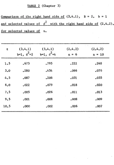
Remark 5 . Table 2 in Appendix 1 compares the result of Dubins and

Savage ([4], or Theorem 2.4.2) with (1) for selected values of

b, d^ , and B 5 and shows how (2.4.2) is improved in B ’.

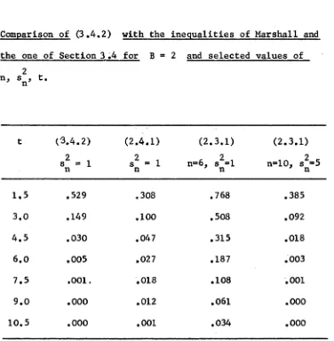
Table 3 in the same appendix compares. Marshall's result ([14],

or Theorem 2.4.1) and (2.3.1), the analogous result of Chapter 2,

with (1) for selected values of n, s2 , and t, and shows how n

they can be improved in V(n).

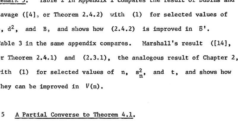
§5 A Partial Converse to Theorem 4.1.

The proof of Theorem 4.1 used (3.7), which bounds moment generating

functions of elements of 3. It is interesting that the conclusion

of Theorem 4.1, itself provides a bound for moment generating functions

of elements of M(n) - a partial converse to "(3.7) implies

[image:49.549.92.493.269.487.2]

Theorem 1 . Take n e I+ 5 {S^} c M (n) and numbers b, d2 , B such

that 0 < b < V(S |S S„) = C2 < d2 almost surely. If (4.1)

---- — n 1 n-1 i n — --- *

---holds for {S^} then {S^} e 3 and for each K > 0.

(1) E(exp(kS^)) <_ exp(Wk2 ) |kj <_ K

where the constant W is independent of k .

Proof: The statements

oc

(2) E(exp(kS )) = / e^X dPr(S < x}

n n —

= 1 + / (ekx-kx-l)dPr{S < x)

J n —

— 00

< 1 + 1/2 / k 2x 2e ^ X dPr(S < x}

— J „ n —

follow from definition, {S_^} e ^ (n ) j and the easily established

inequality e ^ - kx - 1 <_ (k2x 2e ^ X )/2, respectively. Because

(4.1) holds for (S^), we have, setting u = td2

(3) Pr(IS I > u) < 2Pr(M > uC2 /d2 }

1 n — — n — n

for u > 0. Integrating (2) by parts yields, after some calculation.

k 2

(4) E(exp(kS ) ) < _ ! + -— - / [2x+x2 |k| ] e ^ XPr{ | S | >. x H x

Using (3) in (4) and |k| <_ K within the integral shows that the integral in (4) exists and equals, say, 2W which proves the theorem because 1 + k 2W < e^ ^ .

CHAPTER IV Some Limit Properties

§ 1 Introduction and Summary.

In this chapter we investigate the problem of bounding elements

of B almost surely. Feller [6] and Chung [3] have studied the

question for sums of independent random variables with zero mean and finite third moment and obtained very precise upper bounds for

(Sn ) and {Hn >, respectively.

Using terminology due to Levy [12] a positive, non-decreasing

sequence of real numbers;, {g^} is said to be in the upper class LI

or the lower class L, with respect to {S_.}, a sequence of

zero-mean random variables whose variances, s2 , exist, if the series

* n ** *

(1) Y Pr{5 > s g }

L n — n n

n

converges or diverges, respectively. The concept is convenient for

describing classical laws of large numbers as well as for investigating

more subtle properties concerning the limiting behaviour of {S^}. For

independent random variables = ±1 almost surely,

(RI) = 0 ( n ^ ^ + ^) almost surely, 6 > 0

1/2

(R2) = 0((nlogn) ) almost surely

1/2

(R3) = O((nloglogn) ) almost surely

due respectively to Hausdorf, Hardy-Littlewood, and Hintchine

merely assert that the sequences {n^}, {(logn)^^^}, { (loglogn)^^} are in

U

with respect to (S }, 6 > 0; (S = 0(g ) => S /g

n 7 n n n n

ultimately bounded),

In Feller [6] the nature of

U

was elucidated, showing precisely what the almost sure upper bounds for sequences {S^} are (where S_.

is the sum of i independent, zero mean random variables whose third moment is finite, i e I+ ) , while Chung extended these results

analogously to {fO for both classes

U

and

L.

The possibilities for further clarification along these lines are thus limited.

Here we adopt a different viewpoint predicated on the fact that while a real sequence {g^} maY be in Ü with respect to {S^},

the random variable S = sup(M /(s g )) will have large values. n n n

Accordingly we shall seek conditions under which a sequence {Sn } e 3

is almost surely bounded in the sense that S has a moment generating

function. Results of this kind will give less precise upper bounds

on {S } than those germane to the upper class though at the same n

time are strong in that they rigidly bound tail probabilities for S.

Specifically for {S^} c 3 we shall say that a positive * non­

decreasing real sequence {g^} is in the class U or

L

with

respect to {S^} according to whether (1) converges or diverges,

respectively. Further, {g^} will be said to belong to the class

S with resDect to {S } e 3 if S = sun M

/ ( / Z C

g ) has a moment

r

n n n n

n

generating function. In Section 2 we give a criterion for membership

in

S

and in Section

3,

for random variables in

I,

the class

U

Pi S is considered. The main result here is that a certain sequence

(gn ), shown by Chung to belong to U, is also in S with respect to

certain {S^} e Finally Section 4 extends some of the preceeding

results to a wider subclass of

B,

§2 A Criterion for Membership in S .

The main result of this section, Theorem 4, depends on the following

Lemma 1 ; Let {S^} e 5» n e I+ , and t > 0 be given. Then

(1) Pr{M >_ t} <_ exp(-t2/(4nB2 )

where B = max B .. l<i<n 1

Proof: By Theorem 1.2.5, since 8 C W ( n ) for all n e I+ ,

(2) Pr{M >_ t} <_ E(exp(kSn ) )/exp(kt)

for all k,t > 0 and, together with (3.3.7) there follows

LP.

(3) Pr{M >_ t) <_ exp((e " -kB-l)d2/B2-kt)

where, as in Section 3.3, d2 denotes a number satisfying d2 > C2 = ( S | S ,,...,8-) almost surely.

— n n 1 n-1* 1 J

kB If k < 1/B a simple estimate for the Taylor series of e'v yields e'^ - kB - 1 <_ 3k2B2 /4. As

^X J - Bi - B? i = !.•••,n 5 V(X ) £ B2 and

(4) Pr{Mn >_ t} <_ exp(3nk2h2 /4 - lex)

where we have used the monotonicity of exp.

Putting k = x/(nB2) in (4) gives (1) which, as (4)

is valid for k < l/B, holds for x < nB. However 1-1 < nB almost

— n —

surely so that (1) is valid for all x > 0.

Given {S^} e B, a number 'C > 0, an increasing sequence of integers, {n.}, and a positive increasing real sequence {g },

3 n

define for each T > 0, the sequence

(

5)

VT

)

= / Pr{ expO^l /( /2n’"g )) > y}dy

T j+1 J j

Theorem 4 will show that the convergence of is intimately related to membership of S. Lemma 1 we obtain

Y a.CT) for some T > 1

b j

3

In preparation, from

Theorem 2. For such that n.,./n.

j+1

3

sequence of reals,

{S^} e Bj {n_.} an lncreasln§ sequence of integers is bounded, and {g } a positive increasing

n

(6) £ [ e x p (-Mg2 /2)]/(Mg2 ) > M > 0

j lj 3

i s s u f f i c i e n t f o r t h e c o n v e r g e n c e o f £ a . ( T ) f o r some T > 1.

.1

1

P r o o f ” F i x j e I . By Lemma 1 , f o r any T > 1 and K > 0

( 7 ) a j W 2L / e x p ( - ( g n ( l o g y ) / ( K B ) ) 2n . / ( 2 n ^ + 1 ) ) d y

Put t . = v n . / n < 1. Put z = t g ( l o g y ) / ( B K ) - BI1

/

( t . g ) i n

3 3 J4-1 3 n • 3

(7 ) t o s e e t h a t

(6) a . (T) <_ K' / e “ z 2 / 2 <

J ij> I

w h ere I'* = BK.(exp(B2K2 / ( 2 t 2 g2 ) ) ) / ( t . g ) and

J n j 3

T* = t . g ( lo g T ) / ( B K ) - B K / ( t . g ) . F i n a l l y from t h e f a m i l i a r

3

nj

-1

nj

e s t i m a t e o f t h e r i g h t hand t a i l o f t h e normal d i s t r i b u t i o n , we have

( 9 ) a . ( T ) £ [ e x p ( - t . g ( l o g T ) / ( B l 0 2 / 2 ) ] T B 2 K2 / ( ( l o g T ) t 2 g2 -B 2IC2 )

2 3 3 1 j

from w h ich t h e c o n v e r g e n c e o f £ a^(T ) i s a p p a r e n t i f T = e x p (B K /m /f)

w h ere f = min t . , and f > 0 by a s s u m p t io n .

Further9 the preceding proof adapts to give

Corollary 3 . If, in addition to the assumptions of Theorem 2 there

is S > C such that c2 g2 almost surely, the convergence of

(6) is sufficient for that of £ b.(T) where j 3

(10) b .(T) = / Pr{exp(KH /(/2C g )) > y}dy

J

T

V l

"j "j

Proof; Lemma 1 gives for j e I+

(11) b.(T) < / exp(-(logy)2g2 C 2 / (2K2B 2n.+ 1 ))dy

3 T nj n j 3

whence, as C 2 > n.£2 almost surely, b.(T) is no more than

n . — j j

3

(12) / exp(-(g £(logy)/(KB))2t./2)dy

T j 3

With z = t g 5 (logy)/KB - KB/(fit g ) in (12),

3 j 3 j

t_. = /n_. /n ^ as before, the obvious estimate of the resulting integral

gives

(13) b . (T) < [exp(-g t.Ä(logT)/(3IC))2 /2]TB2K2 /((logT)t.g2 ^ - B 2 «2 )

~ n. 2 i n .

and the assertion is obvious when T = exp (;/m3K/(£f ) ) , f = min t..

j 3

With the help of Corollary 3 we can give a condition sufficient

for {g } e S which will be useful in what follows, n

Theorem 4 For {S } e 0 if there is

6 >

0 such that c

2 > 6

--- n n —

almost surely, {n^ } is as in Theorem 2, and {g^} is a positive,

non-decreasing sequence for which (6) converges, then {g^} e 5

with respect to {S^}.

Proof: For S = sup M / (/2C g ) and k > 0

--- n n n

n

(14) E(exp(kS)) =

J

y d?r{exp(kS)

<_

y)

0

<_

j

Pr{exp(kS) > y}dy

0

and thus it suffices to demonstrate the existence of T > 1 for

00

which

j

Pr{exp(kS) > y}dy is finite. T

The event (S >_ t} is contained in the event

{M, / (/2C g ) > t for some k < n.,-} where, without loss

k n. n. — — j+1 *

3=0 j j