https://doi.org/10.1007/s40890-019-0075-7 ORIGINAL ARTICLE
Car Trip Generation Models in the Developing World: Data Issues
and Spatial Transferability
Andrew Bwambale1 · Charisma F. Choudhury1 · Nobuhiro Sanko2
Received: 21 July 2018 / Accepted: 22 March 2019 © The Author(s) 2019
Abstract
In many countries of the developing world, it is difficult to conduct large-scale household travel surveys to collect data for travel behaviour model estimation and application. This paper focuses on two candidate solutions to the problem: (1) developing models that can be applied for prediction using secondary data collected for other purposes and include socio-demographic information but do not include transport specific information such as the car and/or transit pass ownership (e.g. census, public health records, etc.), (2) ‘borrowing’ a model developed using data from a similar city within the same region. In the first approach, we investigate the feasibility of developing car trip generation models which imputes the car ownership variable with estimated car ownership propensities. The proposed framework is applied in two East African cities, Nairobi and Dar-es-Salaam. The estimation results indicate that for both cities the proposed approach outperforms the models that exclude the car ownership variable. In the second approach, we investigate the spatial transferability of the models developed in the first approach between the two cities to evaluate if it is justified to apply models from one developing country to another in the absence of local models. Results indicate that though some of the estimated parameters are not significantly different from each other between the two cities, statistical tests do not support direct transferability of all the models from Nairobi to Dar-es-Salaam or vice versa. However, interestingly, the simpler model (which excludes car-ownership) outperforms the model with imputed car ownership propensity in terms of transferability. These findings provide useful insights into the development of trip generation models under data constraints which can practically be very useful for developing countries.
Keywords Car ownership · Trip generation · Travel behaviour · Nairobi · Dar-es-Salaam
Introduction
In recent years, developing countries have witnessed speedy urbanisation, improvements in living standards and sig-nificant growths in economic activities. As a consequence, there has been a substantial increase in disposable household income levels [8] which has led to a significant increase in car
ownership levels in most of the countries. The increased car ownership levels, coupled with increased economic activities, have led to an increase in the overall numbers of car trips, which has contributed to increased traffic congestion, energy consumption, and air pollution, particularly in big cities [10].
Given the important role of the trip generation compo-nent in transport planning, there has been numerous research studies investigating the relative contribution of different factors on trip generation [1, 15, 32, 38, 44]. However, these studies are conducted in the context of developed countries, and the findings as well as the methodologies are not directly applicable to developing countries due to substantial differ-ences in the socio-economic conditions and data issues. Trip generation studies in developing countries on the other hand are still limited, primarily due to the lack of data for calibrat-ing and applycalibrat-ing the trip generation models. But there are often secondary datasets available in developing countries, which have detailed socio-demographic information (e.g. census, public health records, etc.). However, in most cases
* Charisma F. Choudhury
[email protected] Andrew Bwambale [email protected] Nobuhiro Sanko [email protected]
1 Institute for Transport Studies, University of Leeds,
Leeds LS2 9JT, UK
2 Graduate School of Business Administration, Kobe
they lack car ownership information—which has been found to be a critical variable in trip generation models. Although there are examples of trip generation models without the car ownership explanatory variable in the context of develop-ing countries (e.g. [42], there is a substantial risk that this introduces a strong correlation between the error term of the model and the rest of the explanatory variables. Such omission can, therefore, lead to endogeneity and bias in the estimates [43]. Consequently, it is critical that the relation-ship between trip generation and car ownerrelation-ship, as well as the influence of other exogenous factors, is well represented to mitigate the endogeneity problem.
Furthermore, the relationship between car ownership and trip generation is more complex than usually presented. While ownership of car offers increased flexibility and mobility, people with increased mobility needs are likely to be more prone to own cars (provided that they can afford). This can lead to potential simultaneity between the two deci-sions and can lead to endogeneity, where an explanatory variable (car ownership) is influenced by the dependent variable (trip generation) [43]. Where attempts have been made to address this issue, it has been hypothesised that current car ownership is influenced by trip generation from a previous period, reflecting the “learning from experience idea” [26]. The development or application of such mod-els, however, requires panel data, which are difficult to find in developing countries since there is rarely any initiative to systematically document travel survey records [36]. To the best of our knowledge, there has not been any previous research that investigates how a robust and dependable trip generation model can be developed in the context of devel-oping countries amid these data limitations.
On the other hand, ‘borrowing’ models from similar set-tings also hold the promise for overcoming the issues arising from the absence of dependable travel behaviour data for developing local models. But though there has been substan-tial research on transferability of models developed for one location to another in the context of developed countries (see [40] for a detailed synthesis), this has not been investigated rigorously in the context of developing countries.
In this research, we address these research gaps in the following two ways:
• exploring candidate model structures to address the issue of unavailability of a key variable in the application con-text (car ownership in this case);
• investigating the spatial transferability of these model structures to evaluate if it is justified to apply models from one developing country to another in the absence of local models.
The models are estimated using household survey data collected from two East African cities, Nairobi, Kenya,
in 2004 [22], and Dar-es-Salaam, Tanzania, in 2007 [23]. Given their geographical proximity, similarities in their socio-economic structure, and their fairly similar transport systems [21], it is expected that there will be some similari-ties in the travel behaviour of the two cisimilari-ties, which prompts us to investigate the spatial transferability of the models between the two cities.
In this regard, two different model structures (i.e. one sequential and one simultaneous structure) are developed and their performances are compared against models where all the variables are observed. The spatial transferability of each of these model structures is then tested to investigate which one is more transferrable to the other city. It may be noted that we focus on car trips (as opposed to the total num-ber of trips) because private cars are the key contributors to congestion in both cities [22, 23].
The rest of the paper is arranged as follows: a review of literature on trip generation, vehicle ownership models and spatial transferability are presented first. This is followed by a description of the modelling methodology and the details of the data for each city. The empirical findings are pre-sented next, followed by the key findings and directions for future research.
Literature Review
This section briefly reviews literature on trip generation and car ownership models and that on spatial transferability of models.
Previous Trip Generation and Car Ownership Studies
In the case of car ownership, household income and the number of driving licence-holding members have been found to have a consistent positive influence on the number of cars owned by a household [31]. The other key household socio-economic/demographic exogenous factors previously considered to affect car ownership include household size, number of children, accessibility measures [31]; the number of workers in a household [7, 14, 33, 37–39], age and gender of the household members [37], and family structure [7, 14,
33]. Aggregate variables such as population density [24, 38,
45] and residential density [33, 39] have also been previ-ously considered as explanatory variables.
Most of the previous studies encountered in this field have employed discrete choice methods in estimating car ownership [7, 14, 26, 31, 37, 39, 45] and trip generation [1,
32]. Obviously, there are other studies that have used dif-ferent techniques such as linear regression [24, 38, 42] and structural equations [19, 20], but discrete choice methods are more appropriate for this study since they are able to represent a decision maker’s choice from a set of discrete alternatives, where at least one and only one can be chosen at a time [6].
Based on the sample studies above, it is noted that both car ownership and trip generation largely depend on similar explanatory variables. As earlier mentioned, this points to the fact that arbitrary omission of the car ownership vari-able in trip generation models increases the risk of endo-geneity due to variable omission [43]. That aside, this is also used to our advantage in scenarios where there is lack of car ownership data in the application context, without needing a new set of explanatory variables. A possible way is provided in a study [38] where the influence of vehicle ownership is incorporated into a ‘vehicle use model’ using a separately estimated vehicle ownership model based on a largely similar set of explanatory variables. The setback is that this study uses linear regression models which are not suitable for developing disaggregate car ownership or car trip generation models.
Structures of State‑of‑the‑Art Trip Generation and Car Ownership Models
Most previous studies have used discrete choice methods for modelling car ownership and trip generation decisions due to the discrete nature of the explanatory variables. Dis-crete choice models can generally be divided into unordered response or ordered response models. Depending on the nature of the study, previous vehicle ownership studies have used both unordered [7, 14, 33, 45] and ordered [7, 29, 31,
37, 39] response models, while most previous trip generation studies have used ordered response models [1, 32].
Although it is possible to use both unordered and ordered response models, car ownership level and trip
generation choices are incremental by nature which makes ordered response models more appropriate. Modelling these as ordered choices means acknowledging that there is a correlation between the alternative choices for each case (See [6] for details). With ordered response mod-els, it is also possible to conduct multivariate analysis for cases with more than one dependent variable [35]. This has previously been used to jointly model household car and motorcycle ownership levels in Asia using bivariate ordered response probit (BOP) models [37]. However, to the best of our knowledge, no previous study has inves-tigated the possibility of jointly modelling car ownership and car trip generation using the BOP model, and this study addresses this research gap among others.
Spatial Transferability of Trip Generation and Car Ownership Models
From the onset, we highlight the difference between model transfer and transferability, with the former simply being an act of transferring models between contexts and the latter being the degree of success with which a model esti-mated for a given context explains behaviour in another context [34].
Transferability can be investigated between different time periods within the same area (temporal transferabil-ity) or between different geographical areas (spatial trans-ferability) or both [1, 9, 17, 40]. Previous studies have established that spatial transferability of trip generation [1, 11, 34, 41, 42] and car ownership [37] models can be reasonably achieved. This is, however, is not always the case; for example, in a study [13], satisfactory spatial transferability of trip generation was not achieved on an account of underlying differences between London and Tel-Aviv city structures.
Transferability improves when models are developed at a disaggregate level [30]. It has been argued that pref-erence for disaggregate models is due to the observation that they do not depend on unique zone definitions [42]. It is, however, difficult to achieve flawless model transfer-ability and, therefore, the aim usually is to make as much improvement in transferability as possible [27].
Methodology
Based on the review of literature (“Structures of State-of-the-Art Trip Generation and Car Ownership Models”), we use ordered response models which assume that every indi-vidual has latent car ownership and trip making propensities which are functions of their demographics. These propensi-ties are then converted to discrete car ownership levels and trips using estimated cut-off points.
Model Structures
The model system consists of two submodels, one for car ownership, and the other for trip generation.
Car ownership submodel:
Trip generation submodel:
where y∗1n and y∗2n are the car ownership and trip generation
propensities, respectively, for household n ; x1n and x2n are
vectors of the car ownership and trip generation explana-tory variables, while 𝛽1 and 𝛽2 are the respective parameter
vectors. y1n is the observed car ownership for n , which is
different from y∗
1n , the estimated car ownership propensity. y2n denotes the observed car trips for n . The corresponding
parameters 𝛾 and 𝜆 are mutually exclusive depending on the
model being estimated as described in the next paragraph. The 𝜇 s are the threshold parameters.
The three models estimated below are expressed as spe-cial cases of the two submodels.
Base model This model is applicable for the case where car ownership data are available, and the number of cars owned ( y1n ) is directly used as an explanatory variable.
Hence, in the model formulation, Eqs. (1c) and (1d) are used and, 𝛾 is estimated, but 𝜆 is fixed to zero. A variation
of the model without the car-ownership variable has been tested as well.
Sequential model This model accounts for situations where car ownership data are available in the estimation context but missing in the application context, and attempts (1a)
y∗1n=𝜷�1x
1n+𝜀1n,
(1b)
y1n= ⎧ ⎪ ⎨ ⎪ ⎩
0 if y∗
1n≤𝜇1,0, 1 if𝜇1,0<y∗
1n≤𝜇1,1, 2 if𝜇1,1<y∗
1n≤𝜇1,2, 3+ if𝜇1,2<y∗
1n.
(1c)
y∗ 2n=𝜷
�
2x2n+𝛾y1n+𝜆y∗1n+𝜀2n,
(1d)
y2n= ⎧ ⎪ ⎨ ⎪ ⎩
0 if y∗2n≤𝜇2,0, 1 if𝜇2,0<y∗
2n≤𝜇2,1,
2 if𝜇2,1<y∗
2n≤𝜇2,2,
3+ if𝜇2,2<y∗
2n,
to address this issue using the estimated car ownership pro-pensity.1 In this formulation, the car ownership submodel
(Eqs. (1a) and (1b)) is estimated followed by the trip genera-tion submodel (Eqs. (1c) and (1d)). The car ownership pro-pensity y∗
1n is derived from the car ownership submodel y ∗ 1n
and utilised in the trip generation submodel; 𝜆 is estimated,
and 𝛾 is fixed to zero.
For the base and the sequential models, the car ownership and the trip generation probabilities can be estimated using the ordered response probit model as follows:
where 𝛷(⋅) is a standard normal cumulative distribution
function, and Pn,y
a is the probability of household n falling
in category ya ; a = 1 for the car ownership submodel, and 2
for the trip generation submodel.
The models are estimated using the maximum likeli-hood estimator. Equation (2b) presents the log-likelihood function:
where Zn,y
a=1 if and only when household n is in category ya and 0 otherwise. It may be noted that for the base model,
we only estimate the trip generation submodel, while for the sequential model, we sequentially estimate the car ownership and the trip generation submodels.
Simultaneous model In this model, the car ownership and the trip generation submodels are estimated jointly. This model thus attempts to address the simultaneity problem between car ownership and trip generation, as well as car ownership data shortages in the application context. Here again, the car ownership propensity y∗
1n is calculated in the
car ownership submodel and utilised in the trip generation submodel, where 𝜆 is estimated, and 𝛾 is fixed to zero.
How-ever, the car ownership and the trip generation probabilities are jointly estimated using the bivariate ordered response probit model as follows [35]:
(2a)
Pn,y
a=𝛷
( 𝜇a,y
a−y
∗
an )
−𝛷(𝜇a,y
a−1−y
∗
an )
,
(2b)
LL= N
∑
n=1 Ya
∑
ya Zn,y
a×ln(Pn,ya),
(2c)
Pn,y 1y2 =𝛷
( 𝜇1,y
1−y ∗ 1n,
( 𝜇2,y
2−y ∗ 2n
) 𝜁,̃p)
−𝛷2(𝜇1,y 1−1−y
∗ 1n,
( 𝜇2,y
2−y ∗ 2n
) 𝜁,̃p)
−𝛷2(𝜇1,y 1−y
∗ 1n,
( 𝜇2,y
2−1−y ∗ 2n
) 𝜁,̃p)
+𝛷2(𝜇1,y 1−1−y
∗ 1n,
( 𝜇2,y
2−1−y ∗ 2n
) 𝜁,̃p),
1 Availability of car ownership data in estimation context is less of
where Pn,y
1y2 is the probability of household n owning y1 cars
and making y2 car trips, 𝛷2 a bivariate standard normal
cumulative distribution function, 𝜌 = 𝜁 (𝜆 +̃ corr) ,
𝜁 = √ 1 1+2⋅𝜆⋅corr+𝜆2
, and corr is the correlation between 𝜀1n and 𝜀2n.
Equation (2d) presents the log-likelihood functions for the simultaneous model [35]:
where Zn,y
1y2=1 if and only when household n owns y1 cars
and makes y2 car trips, otherwise it is equal to zero.
An important point worth noting is that for the sequential estimation, only the deterministic component of car ownership propensity is entered in the trip generation model (and used in subsequent forecasting), while for the simultaneous estimation, both the deterministic and the stochastic components of the variable contribute to the model used for forecasting.
Evaluating Spatial Transferability
Three model structures have been specified starting with the base model (the simplest of all), followed by the more complex sequential and simultaneous model structures. Although it is generally assumed that better specified models tend to be more transferrable, this needs to be investigated using the available transferability metrics as it is difficult to assess this from the model specifications alone.
Spatial transferability of the individual parameters is checked by testing whether or not there is a significant differ-ence between the parameter estimates of equivalent variables in the two cities (Eq. 3a) [18]. Minimum and maximum t-ratio values of − 1.96 and 1.96 corresponding to the 95% confidence interval are taken as the critical values:
where 𝛽̂
trans,k and 𝛽̂appl,k are the estimates for the k th
param-eter in the transferred and application areas, ttrans,k and tappl,k
the respective t ratios of the parameter estimates, and tdiff,k is
the t-ratio for the difference between parameters.
Global measures of model transferability are also obtained using the transferability index (TI) (Eq. 3b) [28]:
(2d)
LL= N
∑
n=1 Y2
∑
y2=0
Y1
∑
y1=0
Zn,y
1y2ln(Pn,y1y2),
(3a)
tdiff,k= ̂
𝛽trans,k− ̂𝛽appl,k
√( ̂ 𝛽trans,k
ttrans,k )2
+
(̂
𝛽appl,k tappl,k
)2,
(3b)
TI= LLappl( ̂𝛽trans) −LLappl(C)
LLappl( ̂𝛽appl) −LLappl(C)
,
where LLappl( ̂𝛽trans) is the log-likelihood on the
applica-tion context data with transferred context parameters,
LLappl( ̂𝛽appl) the log-likelihood on the application context
data with application context parameters, and LLappl(C) is
the log-likelihood of the application context model with constants only.
A TI value of one indicates perfect transferability, while a value of zero indicates complete non-transferability. This metric is suitable for comparing the transferability of alter-native model structures; however, there is no specific lower limit to judge whether the reported transferability is good or not. Equation 3b means that a higher LLappl( ̂𝛽trans) always
results in a higher TI.
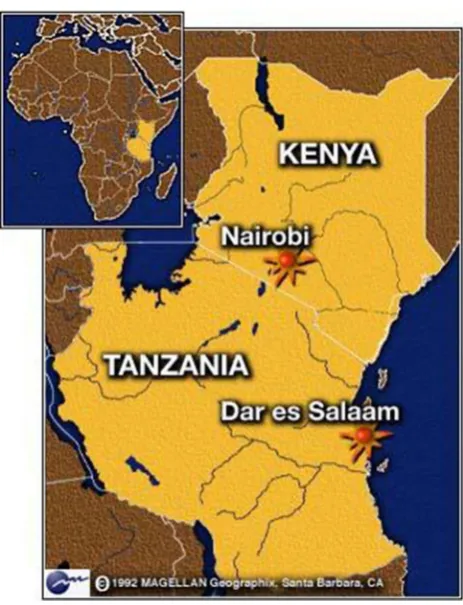
Data
The data used for this study were collected from the cit-ies of Nairobi (Kenya) and Dar-es-Salaam (Tanzania) in 2004 and 2007, respectively. Figure 1 shows the study area locations.
The surveys were conducted by face to face interviews of household members aged 5 years and above (in Nairobi) and 6 years and above (in Dar-es-Salaam). A total number
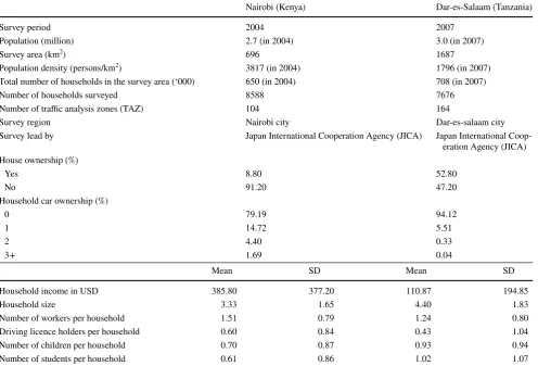
[image:5.595.309.541.53.356.2]of 8588 and 7676 valid household observations were made in Nairobi and Dar-es-Salaam representing sampling rates of approximately 1.3% and 1.1%, respectively. Table 1 pre-sents a brief description of the data while Fig. 2 presents variation of household car trip generation rates with key household descriptors. Though the trends are not identical, in general, the possibility of households making increased numbers of car trips increases with household car owner-ship, household income, the number of licence holders and the number of workers in both cities (Fig. 2a–d). From Fig. 2a in particular, it may be noted that there is a small proportion of households that reported that they do not own a car and yet had car trip origins. This could be because they had access to office cars for work (and for private usage as well in some cases) which are not reported in the numbers of cars owned. These trends are all in agreement with intuitive reasoning. A high number of cars owned are likely to increase the possibility of car use. High income is expected to be highly correlated with high disposable income for spending on private car travel. A high number of driving licence holders would most likely increase the
possibility of the available cars being driven. High num-bers of workers in a household are likely to lead to increase household travel activity in general and possibly car trip generation rates in particular. The other explanatory vari-ables considered to be important are household size and house ownership.
Apart from private car trips, the mode share of walk-ing trips is approximately equal to that of public transport, which is largely under private control in both cities [22]. Public transport in Nairobi comprises of both large buses and minibuses (matatus), while that in Dar-es-Salaam largely comprises of minibuses; however, both cities had no option for rail transport at the time of data collection.
Although public transport is privately controlled, there is a fare setting procedure for large buses and minibuses in both cities, which is managed by transport operator associa-tions [21]. However, public transport operations are largely flexible, with no adherence to departure timetables, which could be one of the issues discouraging high-income indi-viduals from using public transport in both cities.
Table 1 Brief description of the data
Nairobi (Kenya) Dar-es-Salaam (Tanzania)
Survey period 2004 2007
Population (million) 2.7 (in 2004) 3.0 (in 2007)
Survey area (km2) 696 1687
Population density (persons/km2) 3817 (in 2004) 1796 (in 2007)
Total number of households in the survey area (‘000) 650 (in 2004) 708 (in 2007)
Number of households surveyed 8588 7676
Number of traffic analysis zones (TAZ) 104 164
Survey region Nairobi city Dar-es-salaam city
Survey lead by Japan International Cooperation Agency (JICA) Japan International Coop-eration Agency (JICA) House ownership (%)
Yes 8.80 52.80
No 91.20 47.20
Household car ownership (%)
0 79.19 94.12
1 14.72 5.51
2 4.40 0.33
3+ 1.69 0.04
Mean SD Mean SD
Household income in USD 385.80 377.20 110.87 194.85
Household size 3.33 1.65 4.40 1.83
Number of workers per household 1.51 0.79 1.24 0.80
Driving licence holders per household 0.60 0.84 0.43 1.04
Number of children per household 0.70 0.87 0.93 0.94
[image:6.595.52.549.72.409.2]Results
Estimation Results
The estimates and the summary statistics for all the three model structures are presented in Tables 2 and 3, respec-tively. In addition to the three models, we estimated the base model (without the car ownership variable) for comparison purposes. The summary statistics of these models are pre-sented in Table 3.
Positive parameter estimates imply that an increase in any of these explanatory variables increases the propensity of household car trip generation or ownership, while the reverse is true for negative parameter estimates. The same interpretation applies to the relative parameter magnitudes of the dummies associated with the same explanatory vari-able. For all the three models, most of the parameter signs and relative magnitudes are in agreement with intuitive rea-soning. One of the exceptions is parameters associated with the number of workers per household in the car ownership submodels of the sequential and the simultaneous models in both cities, indicating that households with more working members sometimes have fewer cars. The reason for this unusual behaviour needs further investigation; however, a possible interpretation is that household income is much more important and the total number of working members may include low-income workers (who do not contribute to the car ownership). The other exceptions relate to the rela-tive magnitudes of parameters associated with the number of workers per household (for the trip generation submodel of the sequential model in Dar-es-Salaam), and the number of cars owned per household (for the base model in both cities). The estimates do not have a monotonically increasing trend with respect to the number of workers or cars owned. How-ever, this problem is not found in the simultaneous model, thereby supporting its theoretical superiority.
The scalar quantity ‘lambda’ in the sequential and the simultaneous models, which relates the household car own-ership propensity to household car trip rates, is positive as expected. However, it is noted that whereas ‘lambda’ is sig-nificant in Nairobi, it is insigsig-nificant in Dar-es-Salaam. One interpretation is the poorer model fit of the car ownership submodel in Dar-es-Salaam, due in part to more unevenly distributed car ownership such as extremely larger share of 0 car household (see Table 1). However, it is good to keep this since this is a key variable in the present research. Similarly, the correlation parameter (corr) in the simultaneous model is positive in both cities, signifying a positive correlation between household car ownership propensity and household car trip generation as expected.
For model comparison in terms of the measures of fit, we separately analyse the car ownership and the trip generation
submodels since some model structures have both sub-models, while others do not. For the sequential model, the convergence log-likelihoods of the two submodels are determined in a straightforward manner; however, for the simultaneous model, which reports the joint car ownership/ trip generation probabilities, the convergence log-likelihoods of the different submodels need to be computed outside the estimation process. To do this, we sum the joint car owner-ship/trip generation probabilities along the number of trip dimensions (for the trip generation submodel), and along the number of car dimensions (for the car ownership submodel). For example, to obtain the probability of making 0 trips, we sum the joint probabilities of (0 cars, 0 trips), (1 car, 0 trips), (2 cars, 0 trips) and (3+ cars, 0 trips), while to obtain the probability of owning 0 cars, we sum the joint prob-abilities of (0 cars, 0 trips), (0 cars, 1 trip), (0 cars, 2 trips) and (0 cars, 3+ trips). We then apply these unconditional probabilities to the appropriate version of the log-likelihood function in Eq. (2b).
A comparison of the trip generation submodels in terms of the adjusted rho-square values shows that the sequential and the simultaneous models perform worse than the base model containing the observed car ownership variable. This is because the base model uses actual car ownership levels which are not subject to estimation errors such as the latent car ownership propensities in the sequential and the simul-taneous models. This might also relate to the discrete nature of the relationship between car ownership and usage. The dummy coding in the base model shows that the difference in the parameter estimates between 0 and 1 car(s) owned is much higher than those between 1 and 3+ car(s). This sug-gests that although people might use company cars or used cars as passengers, households without cars are likely to use cars less frequently. A dummy coding used in the base model is appropriate to express this, but a continuous vari-able expressed by latent propensity to car ownership is less suitable in this regard. However, both the sequential and the simultaneous models outperform a version of the base model where the car ownership variable is totally excluded, espe-cially in Nairobi where the differences in the convergence log-likelihoods are more pronounced. This signifies that the inclusion of latent car ownership propensity is better than total exclusion of the car ownership variable.
Table 2 Es timation r esults Var iable Base model Seq uential model Simult aneous model Nair obi Dar -es-Salaam t-s tat. diff Nair obi Dar -es-Salaam t-s tat. diff Nair obi Dar -es-Salaam t-s tat. diff Es t. Z ≈ t -s tat. aEs t. Z ≈ t -s tat. aGalbr ait h (1982) Es t. Z ≈ t -s tat. aEs t. Z ≈ t -s tat. aGalbr ait h (1982) Es t. Z ≈ t -s tat. aEs t. Z ≈ t -s tat. aGalbr ait h (1982)
Household car o
wnership submodel
Mont
hl
y
household income (‘000) US dollars
1.942 37.47 0.719 8.24 12.06 1.956 37.73 0.709 8.17 12.34 House o wn -ership 0.490 9.39 0.234 3.54 3.04 0.480 9.17 0.240 3.66 2.87 Dummies r elated t
o number of w
or
kers per household
N
umber of work
-ers = 1 − 0.335 − 2.96 − 0.355 − 3.64 (0.13) − 0.364 − 3.27 − 0.362 − 3.79 (− 0.01) N
umber of work
-ers = 2 − 0.402 − 3.52 − 0.296 − 2.83 (− 0.69) − 0.458 − 4.07 − 0.316 − 3.07 (− 0.93) N
umber of work
-ers = 3 and abo ve − 0.299 − 2.41 − 0.280 − 1.99 (− 0.10) − 0.354 − 2.88 − 0.292 − 2.10 (− 0.33) Dummies r elated t
o number of dr
iving license holders per household
N
umber of driving license hold
-ers = 1 or 2 1.249 24.51 1.468 21.44 − 2.57 1.229 23.94 1.441 21.20 − 2.48 N
umber of driving license hold
-ers = 3 1.525 14.11 1.913 14.55 − 2.28 1.487 13.77 1.885 14.33 − 2.34 N
umber of driving license hold
Table 2 (continued) Var iable Base model Seq uential model Simult aneous model Nair obi Dar -es-Salaam t-s tat. diff Nair obi Dar -es-Salaam t-s tat. diff Nair obi Dar -es-Salaam t-s tat. diff Es t. Z ≈ t -s tat. aEs t. Z ≈ t -s tat. aGalbr ait h (1982) Es t. Z ≈ t -s tat. aEs t. Z ≈ t -s tat. aGalbr ait h (1982) Es t. Z ≈ t -s tat. aEs t. Z ≈ t -s tat. aGalbr ait h (1982) N
umber of driving license hold
-ers = 5 and abo ve 1.861 6.95 2.751 16.61 − 2.83 1.740 6.65 2.726 16.57 − 3.19 Dummies r elated t
o household size
Household size
= 2 or 3 0.096 1.30** 0.384 1.10** (− 0.81) 0.070 0.96** 0.322 0.99** (− 0.76)
Household size
= 4 0.246 3.21 0.470 1.34** (− 0.62) 0.226 2.98 0.400 1.23** (− 0.52)
Household size
= 5+ 0.306 3.97 0.484 1.39** (− 0.50) 0.298 3.92 0.431 1.34** (− 0.40) Thr eshold v alues 0 cars 2.466 19.37 2.757 7.88 (− 0.78) 2.428 19.43 2.680 8.25 (− 0.73) 1 car 3.914 29.29 4.527 12.46 (− 1.59) 3.846 29.33 4.363 12.94 (− 1.43) 2+ cars 4.894 34.87 5.491 13.31 (− 1.37) 4.729 34.42 5.196 13.62 (− 1.15)
Household car tr
ip g ener ation submodel Mont hl y
household income (‘000) US dollars
1.121 19.32 0.290 2.81 7.03 0.846 4.31 0.256 1.25** 2.08 0.954 4.53 0.345 1.66* 2.06 Dummies r elated t
o number of w
or
kers per household
N
umber of work
-ers = 1 0.090 0.60** 0.540 2.89 (− 1.88) 0.126 0.86** 0.524 2.74 (− 1.65) 0.173 1.07** 0.637 2.54 (− 1.55) N
umber of work
-ers = 2 0.519 3.45 0.707 3.73 (− 0.78) 0.494 3.39 0.655 3.55 (− 0.69) 0.618 3.80 0.797 3.23 (− 0.60) N
umber of work
Table 2 (continued) Var iable Base model Seq uential model Simult aneous model Nair obi Dar -es-Salaam t-s tat. diff Nair obi Dar -es-Salaam t-s tat. diff Nair obi Dar -es-Salaam t-s tat. diff Es t. Z ≈ t -s tat. aEs t. Z ≈ t -s tat. aGalbr ait h (1982) Es t. Z ≈ t -s tat. aEs t. Z ≈ t -s tat. aGalbr ait h (1982) Es t. Z ≈ t -s tat. aEs t. Z ≈ t -s tat. aGalbr ait h (1982) Dummies r elated t
o number of dr
iving license holders per household
N
umber of driving license hold
-ers = 1 or 2 0.927 15.79 0.716 8.17 2.00 0.727 5.63 0.645 1.77* (0.21) 0.821 5.95 0.674 1.84* (0.38) N
umber of driving license hold
-ers = 3 1.333 11.55 1.042 6.68 (1.50) 0.958 5.07 0.967 1.98 (− 0.02) 1.078 5.43 1.065 2.23 (0.03) N
umber of driving license hold
-ers = 4 1.764 9.99 1.057 7.55 3.14 1.177 4.78 1.031 1.72* (0.22) 1.362 5.28 1.128 1.88* (0.36) N
umber of driving license hold
-ers = 5 and abo ve 2.116 6.73 1.564 8.38 (1.51) 1.414 3.80 1.525 2.19 (− 0.14) 1.500 4.02 1.669 2.48 (− 0.22) Dummies r elated t
o number of cars o
wned per household
N
umber of car owned
= 1 1.287 25.71 1.543 17.54 − 2.53 N
umber of car owned
= 2 1.523 19.7 1.364 5.44 (0.61) N
umber of car owned
= 3 and abo ve 1.222 10.91 2.366 3.06 (− 1.46) Car o
wnership scalar q
Table 2 (continued) Var iable Base model Seq uential model Simult aneous model Nair obi Dar -es-Salaam t-s tat. diff Nair obi Dar -es-Salaam t-s tat. diff Nair obi Dar -es-Salaam t-s tat. diff Es t. Z ≈ t -s tat. aEs t. Z ≈ t -s tat. aGalbr ait h (1982) Es t. Z ≈ t -s tat. aEs t. Z ≈ t -s tat. aGalbr ait h (1982) Es t. Z ≈ t -s tat. aEs t. Z ≈ t -s tat. aGalbr ait h (1982) Cor relation coefficient cor r 0.043 0.414** 0.295 1.128** (− 0.90) Thr eshold v alues 0 tr ips 2.858 18.89 3.116 16.96 (− 1.09) 2.892 20.16 3.145 14.56 (− 0.98) 3.381 19.61 3.929 7.17 (− 0.95) 1 tr ip 3.689 23.84 3.256 17.60 (1.80) 3.605 24.66 3.256 15.02 (1.34) 4.212 23.79 4.072 7.28 (0.24) 2+ tr ips 4.579 28.91 3.932 20.32 2.59 4.429 29.58 3.802 17.19 2.35 5.128 28.13 4.746 7.76 (0.60) (xxxx) t ratio f or t he differ ence be tw een par ame ters [ 18
] is less t
han 1.96 in absolute ter
ms
Dummies f
or t
he number of cars o
wned per household ar
e r
elated t
o “g
amma” in Eq. (
1c
) and T
able
2
* Insignificant at t
he 95% confidence le
vel but significant at t
he 90% confidence le
vel
** Insignificant at t
he 90% confidence le
vel
a For
lar
ge
n
, z-s
tatis
tic is appr
oximatel y eq ual t o t he t-s tatis tic Table 3 Measur
es of fit
LL(F) con ver gence log-lik elihood, LL(C) log-lik
elihood at sam
ple shar es, LR lik elihood r atio Model s tructur e Model/submodel
No. of parame
ters
Nair
obi, 8588 households
Dar
-es-Salaam, 7677 households
Cr itical chi-sq uar e value LL (C) LL (F) LR Adj-r ho sq uar e LL (C) LL (F) LR Adj-r ho sq uar e
Base model (wit
h t he car o wnership v ar i-able) Joint model – – – – – – – – – – Car o wnership – – – – – – – – – – Tr ip g ener ation 11 − 6030.70 − 3369.59 5322.22 0.4389 − 1543.36 − 946.41 1193.90 0.3865 19.68
Base model (wit
hout
the car o
data, where households are investigated over a given period of time as this would reveal more behavioural aspects of the car ownership/trip generation relationship.
Evaluation of Spatial Transferability
The parameter signs for each of the three models are similar across both cities which is an indication of similarities in car ownership and trip generation behaviour. Analysis of the t-statistics for the difference between parameters (headed by ‘t-stat. diff’ in Table 2) reveals that most of the parameter estimates for all the three models have insignificant differ-ences in magnitude which indicates that they are individu-ally transferrable between the two cities. It is noted that the monthly household income parameter is the least transfer-able potentially due to difficulties in categorising the income data for the two cities into equivalent income groups which lead to the use of a continuous income variable.
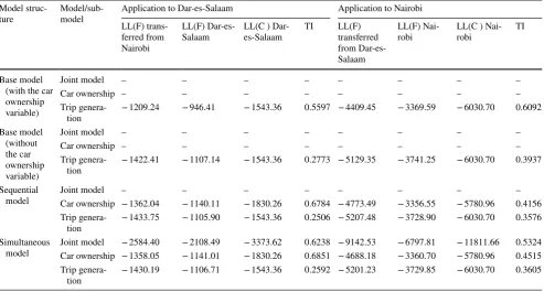
In terms of the overall spatial transferability, Table 4 pre-sents the transferability indices for all the estimated mod-els. Transferability is tested in both directions by applying the Nairobi parameters to the Dar-es-Salaam data (column headed by ‘application to Dar-es-Salaam’) and by applying the Dar-es-Salaam parameters to the Nairobi data (column headed by ‘application to Nairobi’). For each direction, we compare the likelihood ratio of the transferred and the local model with respect to local model having constants only using the transferability index (TI) (see Eq. (3b)). A higher TI indicates higher transferability.
With respect to the trip generation submodel, the base models (both with and without the car ownership variable) produce the highest TI values (the highest LL values with transferred parameters; see Eq. 3b) in both directions com-pared to the rest of the models. The higher transferability of the base models might relate to their simple model structure, which only relies on the observed variables. On the other hand, the sequential and the simultaneous models, which contain a variable that is already subject to estimation errors in the local context (i.e. the car ownership propensity) are likely to perform even worse when transferred as expected.2
The critical point now is the trade-off between local model performance and spatial transferability, when faced with pos-sible data limitations in the application context. In this study, we see that although exclusion of the car ownership variable from the base model structure leads to poor performance in the local context, when compared to models using the
Table 4 Transferability indices
Model
struc-ture Model/sub-model Application to Dar-es-SalaamLL(F) trans- Application to Nairobi ferred from
Nairobi
LL(F)
Dar-es-Salaam LL(C ) Dar-es-Salaam TI LL(F) transferred from Dar-es-Salaam
LL(F)
Nai-robi LL(C ) Nai-robi TI
Base model (with the car ownership variable)
Joint model – – – – – – – –
Car ownership – – – – – – – –
Trip
genera-tion − 1209.24 − 946.41 − 1543.36 0.5597 − 4409.45 − 3369.59 − 6030.70 0.6092 Base model
(without the car ownership variable)
Joint model – – – – – – – –
Car ownership – – – – – – – –
Trip
genera-tion − 1422.41 − 1107.14 − 1543.36 0.2773 − 5129.35 − 3741.25 − 6030.70 0.3937 Sequential
model Joint modelCar ownership − 1362.04– –− 1140.11 –− 1830.26 –0.6784 − 4773.49– − 3356.55– − 5780.96– –0.4156 Trip
genera-tion − 1433.75 − 1105.90 − 1543.36 0.2506 − 5207.48 − 3728.90 − 6030.70 0.3576 Simultaneous
model Joint modelCar ownership − 1358.05− 2584.40 − 2108.49− 1141.01 − 3373.62− 1830.26 0.6238 − 9142.530.6851 − 4688.18 − 6797.81− 3360.70 − 11811.66− 5780.96 0.53240.4515 Trip
genera-tion − 1430.19 − 1106.71 − 1543.36 0.2592 − 5201.23 − 3729.85 − 6030.70 0.3605
2 Model specification is largely driven by the characteristics of the
[image:13.595.52.546.71.336.2]estimated car ownership propensity (i.e. the sequential and the simultaneous models. See Table 3), the base model with-out the car ownership variable is more spatially transferra-ble. This might relate to the choice of explanatory variables. Explanatory variables in the car trip generation submodel (except the car ownership variable) are also included in the car ownership submodel. The contribution of car ownership propensity in the car trip generation submodel consists of these explanatory variables and the other variables included only in the car ownership submodel. If the contribution from the other variables is limited, the base model (without the car ownership variable) might work as a reduced form of the sequential and simultaneous models.
Therefore, for situations where data shortages of particular variables are expected in a different geographical area, and yet the spatial transferability of the models is an important issue, it may be better to develop models excluding those particular variables, although this comes at a risk of endoge-neity due to variable omission. At this point, it is also worth noting that although the complex model structures have been found to be the least transferrable, the better transferability of the simultaneous model over the sequential model implies that although the correlation term was not statistically sig-nificant (see Table 2), the superior correlation structure of the model makes it more transferrable. Alluding to earlier, better specification of the car ownership submodel could lead to different conclusions on the transferability of the complex model structures and needs to be investigated further using alternative datasets with more explanatory variables.
Policy Implications and Concluding Remarks
This study has investigated the feasibility of different model structures aimed at addressing the issue of unavailability of data on a key variable in the application context.
The key findings together with their policy implications are as follows.
• The inclusion of latent variables as a proxy for the miss-ing variables is better than total exclusion of the vari-ables with respect to model fit to the estimation dataset. Models considering endogeneity and simultaneity have stronger theoretical underpinning which is supported by the better goodness-of-fit with the data. In addition, the simultaneous model produced intuitive estimates as men-tioned in “Estimation Results”.
• The similarity in travel behaviour across different cit-ies within the same region (as assessed from the statisti-cally insignificant differences in the parameter values) is encouraging, and shows that we should not rule out the possibility of transferring the models between the cities. In this particular study, we note that while there
is a high risk of endogeneity due to omission of the car ownership variable in both cities, the benefits accrued from the spatial transferability of models excluding the car ownership variable overrides the need to address this limitation through complex model structures. There is a need for further investigations using alternative datasets with more explanatory variables to examine if this find-ing can be generalised.
The results of the current models, however, show some minor inconsistencies with intuitive reasoning in terms of the relative parameter magnitudes of some variables, which are an important topic of future research to ascertain the unique characteristics of the study areas. Also, our com-parison between the sequential and the simultaneous mod-els indicates that accounting for the simultaneity between car ownership and trip generation is not critical for the two cities; however, further investigation is needed (potentially using panel data) to see if this finding can be generalised across other cities of the developing world. Further, in this case, car ownership information has been assumed to be available for model estimation and unavailable in the appli-cation context. However, in more limiting situations, such information may be completely unavailable, which may necessitate the development of hybrid models as a possible direction of future research. Last, in the present study, we use the same model specifications in all three cases for the sake of comparability. It is, therefore, not possible to provide a detailed conceptual or theoretical guidance on the opti-mum model specification based on our empirical findings. This can be a topic of future research where the effect of model specification on transferability is investigated using a larger number of datasets with varying characteristics. It will be also interesting to investigate methods to increase spatial transferability of the models by methods such as Bayesian updating and joint context estimation (e.g. [16]).
Acknowledgements The authors would like to thank JICA for provid-ing the data and technical reports used in this study. The lead author acknowledges the support of the Commonwealth Scholarship Commis-sion for conducting the research.
Open Access This article is distributed under the terms of the Crea-tive Commons Attribution 4.0 International License (http://creat iveco mmons .org/licen ses/by/4.0/), which permits unrestricted use, distribu-tion, and reproduction in any medium, provided you give appropriate credit to the original author(s) and the source, provide a link to the Creative Commons license, and indicate if changes were made.
References
2. Atherton TJ, Ben-Akiva ME (1976) Transferability and updating of disaggregate travel demand models. Transp Res Rec 610:12–18 3. Badoe D, Miller E (1995) Analysis of the temporal transferability
of disaggregate work trip mode choice models. Transp Res Rec 1493:1–11
4. Badoe D, Miller E (1995) Comparison of alternative methods for updating disaggregate logit mode choice models. Transp Res Record 1493:90–100
5. Badoe D, Chen C (2004) Modeling trip generation with data from single and two independent cross-sectional travel surveys. J Urban Plan Dev 130:167–174
6. Ben-Akiva ME, Lerman SR (1985) Discrete choice analysis: theory and application to travel demand. MIT Press, Cambridge 7. Bhat CR, Pulugurta V (1998) A comparison of two alternative
behavioral choice mechanisms for household auto ownership deci-sions. Transp Res Part B 32:61–75
8. Bolt J, Zanden JLV (2013) The first update of the Maddison pro-ject: re-estimating growth before 1820. Maddison-Project Work-ing Paper WP-4, University of GronWork-ingen. https ://www.rug.nl/ ggdc/histo rical devel opmen t/maddi son/publi catio ns/wp4.pdf. Accessed 15 Apr 2019
9. Bowman JL, Bradley M, Castiglione J, Yoder SL (2014) Mak-ing advanced travel forecastMak-ing models affordable through model transferability. 93rd Transportation Research Board Annual Meet-ing, Washington DC, USA
10. Button K, Ngoe N, Hine J (1993) Modelling vehicle owner-ship and use in low income countries. J Transp Econ Policy 27(1):51–67
11. Caldwell LC, Demetsky MJ (1980) Transferability of trip genera-tion models. Transp Res Rec 751:56–62
12. Cotrus AV, Prashker JN, Shiftan Y (2005) Spatial and temporal transferability of trip generation demand models in Israel. J Transp Stat 8:37–56
13. Daor E (1981) The transferability of independent variables in trip generation models. Planning and Transport Res and Comp, Sum Ann Mtg, Proc, 1981 London. PTRC Education and Research Services, Ltd., pp 235–252
14. Deka D (2002) Transit availability and automobile ownership some policy implications. J Plan Educ Res 21:285–300
15. Douglas A (1973) Home-based trip end models—a comparison between category analysis and regression analysis procedures. Transportation 2:53–70
16. Flavia A, Choudhury C (2019) Temporal transferability of vehicle ownership models in the developing world: case study of Dhaka, Bangladesh. Transp Res Rec. https ://doi.org/10.1177/03611 98119 83676 0
17. Fox J, Daly A, Hess S, Miller E (2014) Temporal transferability of models of mode-destination choice for the Greater Toronto and Hamilton Area. J Transp Land Use 7:41–62
18. Galbraith RA, Hensher DA (1982) Intra-metropolitan transfer-ability of mode choice models. J Transp Econ Policy 16(1):7–29 19. Golob TF (1989) The causal influences of income and car owner-ship on trip generation by mode. J Transp Econ Policy 141–162 20. Golob TF, van Wissen L (1989) A joint household travel
dis-tance generation and car ownership model. Transp Res Part B 23:471–491
21. Gwilliam K (2011) Africa’s transport infrastructure mainstream-ing maintenance and management. The International Bank for Reconstruction and Development, The World Bank, Washington, DC
22. JICA (2006) The study on master plan for urban transport in the Nairobi Metropolitan Area in the Republic of Kenya (SDJR06-41). Japan International Co-operation Agency (JICA), Nairobi 23. JICA (2008) Dar-es-Salaam transport policy and system
devel-opment master plan. Japan International Co-operation Agency (JICA), Dar-es-Salaam
24. Kain JF, Beesley M (1965) Forecasting car ownership and use. Urban Stud 2:163–185
25. Karsamaa N, Pursula M (1997) Empirical studies of transferability of Helsinki metropolitan area travel forecasting models. Transp Res Record 1607:38–44
26. Kitamura R (2009) A dynamic model system of household car ownership, trip generation, and modal split: model development and simulation experiment. Transportation 36:711–732
27. Koppelman F, Kuah G, Wilmot C (1985) Transfer model updating with disaggregate data. Transp Res Record 1037:102–107 28. Koppelman FS, Wilmot CG (1982) Transferability analysis of
disaggregate choice models. Transp Res Record 895:18–24 29. Matas A, Raymond JL, Roig JL (2009) Car ownership and access
to jobs in Spain. Transp Res A Policy Pract 43(6):607–617 30. Ortúzar JDD, Willumsen LG (2011) Modelling transport. Wiley,
Hoboken
31. Pendyala RM, Kostyniuk LP, Goulias KG (1995) A repeated cross-sectional evaluation of car ownership. Transportation 22:165–184
32. Pettersson P, Schmöcker J-D (2010) Active ageing in developing countries?—trip generation and tour complexity of older people in Metro Manila. J Transp Geogr 18:613–623
33. Potoglou D, Susilo YO (2008) Comparison of vehicle-ownership models. Transp Res Record 2076:97–105
34. Rose G, Koppelman FS (1984) Transferability of disaggregate trip generation models. In: Proceedings of the 9th international symposium of transportation and traffic theory, pp 471–491 35. Sajaia Z (2008) Maximum likelihood estimation of a bivariate
ordered probit model: implementation and Monte Carlo simula-tions. Stata J 4:1–18
36. San Santoso D, Tsunokawa K (2005) Spatial transferability and updating analysis of mode choice models in developing countries. Transp Plan Technol 28:341–358
37. Sanko N, Dissanayake D, Kurauchi S, Maesoba H, Yamamoto T, Morikawa T (2014) Household car and motorcycle ownership in Bangkok and Kuala Lumpur in comparison with Nagoya. Transp A 10:187–213
38. Schimek P (1996) Household motor vehicle ownership and use: how much does residential density matter? Transp Res Record 1552:120–125
39. Senbil M, Zhang J, Fujiwara A (2007) Motorization in Asia. IATSS Res 31:46
40. Sikder S, Pinjari AR, Srinivasan S, Nowrouzian R (2013) Spatial transferability of travel forecasting models: a review and synthe-sis. Int J Adv Eng Sci Appl Math 5:104–128
41. Walker W, Olanipekun O (1989) Interregional stability of house-hold trip generation rates from the 1986 New Jersey Home Inter-view Survey. Transp Res Rec 1220:47–57
42. Wilmot CG (1995) Evidence on transferability of trip-generation models. J Transp Eng 121:405–410
43. Wooldridge J (2012) Introductory econometrics: a modern approach. South-Western Cengage Learning, Mason
44. Wootton H, Pick G (1967) A model for trips generated by house-holds. J Transp Econ Policy 1(2):137–153
45. Yamamoto T (2009) Comparative analysis of household car, motorcycle and bicycle ownership between Osaka metropoli-tan area, Japan and Kuala Lumpur, Malaysia. Transportation 36:351–366