Correlation and vacancy-flow effects in binary alloys

CORRELATION AND VACANCY-PLOW EFFECTS IN BINARY ALLOYS

Michael John Dallwitz

A thesis submitted for the degree of Doctor of Philosophy- in the Australian National University

work, except where otherwise indicated.

M , 3".

ACKNOWLEDGMENTS

I thank ray supervisors, Dr. A. J. Mortlock and Dr. C. E. Dahlstrom, for encouragement and helpful discussion.

The electron raicroprohe analyses were carried out in the laboratory of the

Bureau

Mineral Resources,

Canberra, and permission to use the equipment was kindly given by Mr. J. M. Rayner, Director, and Dr. N. H. Fisher, Chief Geologist; Mr. W. M. B. Roberts and Mr. R. N. England gave advice on the

operation of the instrument, and on the preparation of specimens for analysis. The use of sputtering for surface preparation was

suggested by Mr. E. Dennis, a fellow research student, and Dr. J. L. McCall, of the Battelle Memorial Institute, Columbus, Ohio, U.S.A. Preprints of papers submitted for publication were provided by Dr. J. R. Manning and Dr. R. 0. Meyer.

Preface.

Introduction to the Theory of Diffusion in Solid Metals.

1. Introduction i

2. Diffusion Equations ii

2.1. Pick's Laws ii

2*2# Tracer Self-Diffusion Coefficients ii

2.3. The Boltzmann-Matano Analysis iv

3. Atomic Theory of Diffusion vii

3.1. Mechanisms of Diffusion vii

3.2. Diffusion as a Random Walk. Correlation Factors viii 3.3. Applications of Correlation Factors xiii

4. Diffusion in a Concentration Gradient xiv

4.1. The Kirkendall Effect xiv

4.2. Darken's Analysis of the Kirkendall Effect X V 4.3. Relation between Tracer and Chemical Diffusion

Coefficients xvii

4.4. Experimental Measurements of the Kirkendall

Part I.

Theoretical Investigation of Correlation Effects in Binary Alloys.

1. Introduction 1

2. Correlation Factors for Diffusion in Pure Cubic,

Tetragonal, and Orthorhombic Crystals 5

2.1. Correlation Factors in Terms of Exchange

Probabilities 5

2.2. Calculation of Exchange Probabilities 9

2.3. Evaluation of Integrals 21

2.4. Conclusions 26

3. Correlation Factors for Diffusion in Unordered

Binary Alloys 27

3.1. Manning's Symmetric Model 29

3.2. Asymmetric Model 34

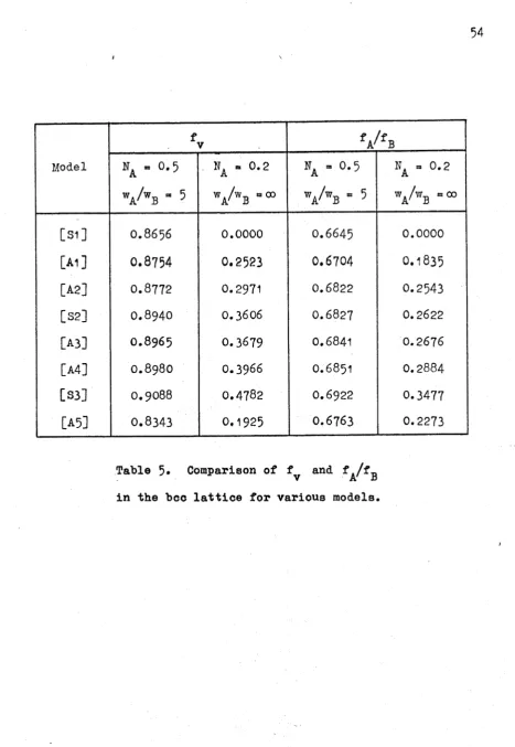
3.3. Comparison of Models 52

3.4. Conclusions 57

Measurement of the Vacancy-Flow Effect in the Interdiffusion of Silver and Gold.

1. Theory 64

1.1. Description of the, Vacancy-Flow Effect 64 1.2. A Parameter Suitable for Accurate

Measurement of the Vacancy-Flow Effect 68 1.3. The Position of the Kirkendall Interface 72 2. Tracer Diffusion Coefficients in Silver-Gold Alloys 74

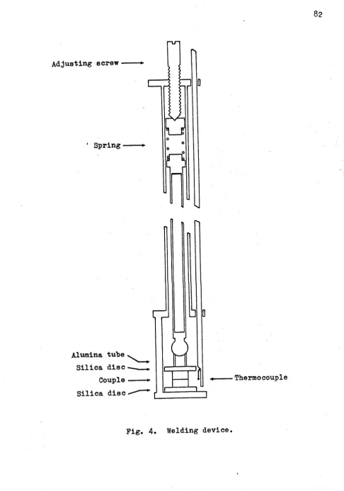
3. Experimental Procedure 80

3.1. Preparation, Welding, and Annealing of

Diffusion Couples 80

3.2. Analysis of Diffusion Couples 87

4. Results 93

4.1. The Kirkendall Interface 93

4.2. Porosity 96

4.3. Numerical Results 98

4.4. The Equilibrium Plane 98

5. Discussion of Results 101

5*1. Quality of Welding 101

5.2. Discussion of Errors 101

% 3 . Results from the Grain-Boundary Interface 102 5.4. Results from Tungsten and Carbon Markers 103 Relation to the Models Discussed in Part I 104 5.6. Comparison with Results of Other Investigations 105

5.7. Conclusions ^07

Symbols Used 108

Experimental Data 110

ABSTRACT.

Part I.

Theoretical Investigation of Correlation Effects in Binary Alloys.

Some improvements are made to the theory of correlation factors for diffusion by the vacancy mechanism in unordered binary alloys. It is shown that earlier estimates of the correlation factors are considerably in error for alloys in which the diffusion of vacancies is highly correlated. Applications to the theory of the vacancy-flow effect are considered.

Part II.

Measurement of the Vacancy-Plow Effect in the Interdiffusion of Silver and Gold.

INTRODUCTION TO THE THEORY OF DIFFUSION IN SOLID METALS.

§1. INTRODUCTION.

The purpose of this preface is to show how the subjects discussed in the main body of the thesis fit into the general framework of diffusion theory, and to provide the necessary background material for readers who are not specialists in the

ii

§2. DIFFUSION EQUATIONS.

§2.1. Fick ’s Laws.

The simplest mathematical description of the diffusion of atoms in solids is based on the assumption that the net flow of atoms is proportional to the concentration gradient, that is,

J = - D grad c , (1)

where J and c are respectively the flux and concentration of the type of atom under consideration, and D is called the diffusion

coefficient. In general, D is a function of the concentration c .

Equation (l) is known as Fick's first law. Applying the continuity

equation

3c

3t - d i v J

we obtain Fick's second law,

^ = d i v ( D grade) . (2)

Equation (2) may be generalized in a number of ways. For

example, D is a scalar quantity only in cubic crystals or in an

isotropic medium; in general, D is a tensor. In this thesis, we

shall mainly be concerned with diffusion in cubic crystals.

§2.2. Tracer Self-Diffusion Coefficients.

By u sing radioactive tracers, it is possible to observe

diffusion in the absence of chemical concentration gradients. In a

a thin layer of a radioactive isotope of the same metal, and the sample is then annealed at constant temperature. After the

annealing, a ’’concentration profile" is obtained by measuring the concentration of the tracer as a function of the distance from the surface.

The diffusion coefficient is obtained from the

concentration profile by making use of the appropriate solution of eqn. (2). Since the chemical composition of the sample is uniform, the diffusion coefficient does not depend on position, and eqn. (2) may be written

3c 3t

t t = D 32

c

where x is the distance from the surface on which the tracer was deposited. It is easily verified that, provided the size of the sample is large compared with the penetration distance of the tracer, the concentration is given by

where A is a constant. This equation may also be written

(3)

In c

2

Hence, if In c is plotted against x , a straight line with gradient l/(4Dt) is obtained. Since the diffusion time t is known, D can be calculated. The diffusion coefficient obtained in this way is called the tracer self-diffusion coeeficient, and is

* denoted by D .

Tracer self-diffusion coefficients can also be defined for diffusion in homogeneous alloys. The tracer self-diffusion

#

iv

coefficient which governs the diffusion of small quantities of tracer i into the alloy.

It is found that the temperature dependence of the tracer self-diffusion coefficients can usually he described by equations

of the form *

D ■ Dq exp (- q/RT)

*

where and Q are constants.

§2.3« The Boltzmann-Matano Analysis.

In another commonly used procedure for measuring diffusion coefficients, a diffusion couple is made by placing two initially homogeneous pieces of metal in contact, and is annealed at constant temperature. The diffusion coefficient, which will, in general, be a function of composition, can be obtained from the concentration profile by a method proposed by Matano (1933)» and based on an analysis by Boltzmann (1894).

Boltzmann showed that if the initial conditions can be expressed in terms of the single variable u = x//t , c is a function of u , and eqn. (2 ) can be transformed into an ordinary differential equation. In the type of diffusion couple described above, the initial conditions are c ** c^ for x < 0 and t * 0 , and c = c^ for x > 0 and t * 0 . In terms of u , these

conditions are c = c at u « -00 , and c « c_ at u =* 00 .

1 2

Using the definition of u , we have

and

3c dc 3u J _ dc

dx m

dx ~

S u b s t i t u t i n g into eqn. (2), we o b t a i n

x dc 3 ( D dc \ 1 d / _ dc \

2t/t du ° 3x \ y t d u / * t du \ d u /

or

u dc d /_ dc \

" 2 du " du T du /

U pon integrating, this e q u a t i o n b e c omes _ I

u dc

du c=c

(4) J c=c.

w h e r e c ’ is a n y c o n c e n t r a t i o n b e t w e e n c^ an d c^ . F o r an y given

c o n c e n t r a t i o n profile, t is constant, and so eqn. (4) m a y be

w r i t t e n

x dc

c*c

c=c c=c

Hence,

D ( c ' ) JL

2t V dc

c=c c

n

x dc (5)

All the q u a n t i t i e s on the r i g h t - h a n d side of this e q u a t i o n can be

measured, and thus D(c') can, in principle, be c a l c u l a t e d for any

c ’ b e t w e e n c 1 and c^ > a l t h o u g h the a c c u r a c y will be p o o r for

vi

Since dc/cbc = 0 when c * c^ , it follows from eqn. (5) that

C2

x dc - 0

°i

§3. ATOMIC THEORY OF DIFFUSION.

§3*1» Mechanisms of Diffusion.

It is well known from the theory of specific heats that atoms in a crystal oscillate around their equilibrium positions. Occasionally these oscillations become energetic enough to allow an atom to change sites. It is these jumps from site to site that give rise to diffusion in solids.

There are several different mechanisms by which these jumps can take place. Some of the most important of these are as follows.

[l] Interstitial mechanism. An atom is said to diffuse by an interstitial mechanism when it passes from one interstitial site to another interstitial site without permanently

displacing any of the atoms on the lattice sites. This mechanism is most likely to occur in the diffusion of small impurity atoms which normally occupy interstitial sites and which can move from one interstitial site to another v/ithout distorting the lattice too much. An example is the diffusion of carbon in iron.

viii

vacancies. If one of the adjacent atoms jumps into the vacancy, the atom is said to have diffused by the vacancy mechanism. It is well established that the vacancy mechanism is the dominant diffusion mechanism in fee metals, and it has been shown to be operative in many bcc and hep metals, as well as in ionic compounds and oxides.

many jumps and traces out an irregular path in the lattice. This is called a random walk. The purpose of this section is to relate random walks to diffusion coefficients; that is, to connect up the atomic and phenomenological theories of diffusion.

[100] or x direction in a cubic lattice. Suppose that initially a large number of tracer atoms are on the (lOO) plane at x = 0 .

After a time t has elapsed, the atoms will be distributed over many (100) planes, and if t is sufficiently large, this distribution may be regarded as continuous. We wish to relate the mean-square

displacement (X ) of the atoms at time t to the diffusion

coefficient. To do this, we note that under the initial conditions described above, eqn. (3) is the solution of Fick’s law. Hence,

§3»2. Diffusion As a Random Walk. Correlation Factors.

Over a period of time, an atom diffusing in a solid makes

Let us consider diffusion by the vacancy mechanism in the

00

p co

_p

<x2 >

=

-00 -CO

*

T h e r e f o r e ,

D

(x //2t

Now

(x~)

2

value of X for a single atom diffusing away from the plane x = 0.

*t ii

For such an atom, let x.. he the x component of the i " jump

between adjacent (lOO) planes. (Jumps within a (100) plane have

zero x component and thus do not contribute to diffusion in the x di r e c t i o n . ) Then

n -i

2

s b < E ’ J >

1=1

n co

lim n-> co

n-1 n-i

“T FTcTÖ

I E W + 2L E

\xi

i=1 n _ _ V "

2t(n)

L_,

i=1 j = 1 oo

( X .2 ) + 2^__ ( * i * 1 + j ) j=1

(6)

Since all jumps between adjacent (100) planes are

crystallographically equivalent and have x components of the same

magnitude,

(x.

write d for the distance between adjacent (lOO) planes and X/ . >,

for the x component of the j * jump following a jump in the +x

direction, eqn. (6) becomes

lim

n-i> oo 2t(n)n)

L

oo 1 +

2r

0=1

1 2

2 * v f

(

7

)

x

and

oo

f

(

₈

)

3=1

v is evidently the average jump frequency for jumps between (lOO) planes, and f is called the correlation factor.

The above equations are also valid for the interstitial mechanism, and similar equations apply for the interstitialcy mechanism. If f = 1 for a particular diffusion mechanism, then diffusion by that mechanism is said to be uncorrelated; otherwise, it is said to be correlated.

The correlation factor f is a measure of the correlation between the directions of jumps in a random walk. If the jump

hence f = 1 . This as the case for the interstitial mechanism, because after an atom has jumped from one interstitial site to

another, it is surrounded by a symmetrical configuration of atoms on lattice sites, and there is no preferred direction for the next jump.

which has just completed a jump is still adjacent to the vacancy which caused the jump, and so the atom has the opportunity of jumping back to its original site. If this happens, the two jumps of the atom are ineffective in causing diffusion of the atom, and so the diffusion coefficient is less than would be expected on the basis of completely random jumps. One way of interpreting this decrease is to regard the term yf in eqn. (7) as the effective jump frequency of the atom, because the diffusion coefficient is directions are all independent, then c= _{0 for all j , and}

frequency v f .

Huntington and Ghate (1962) have suggested a useful and physically meaningful interpretation of correlation effects. The term /x/ . in eqn. (8) is the average x displacement on the j^

'J ' 00

jump following the original jump, and therfore J2, is the average total displacement for the complete sequence of jumps following the original jump.

By considering the symmetry of the configuration after a jump, it is possible to determine whether f is less than, equal to, or greater than 1 for that type of jump. For the interstitial mechanism, the configuration around an atom which has just completed a jump is symmetrical, and therefore the average subsequent

displacement of the atom is 0 , and f = 1 . However, an atom which has just jumped by the vacancy mechanism is surrounded by an

asymmetrical configuration of a vacancy and n -1 atoms, where n

c c

is the coordination number of the lattice. The average subsequent displacement will clearly be towards the vacancy, that is, in the opposite direction to the original jump, and hence f < 1 .

For more complicated types of diffusion where several types of jump (with different frequencies and possibly different jump lengths) contribute to diffusion, it is possible to define a ’’partial” correlation factor for each type of jump. The average subsequent displacement after a jump of a given type is related to the corresponding partial correlation factor by an equation similar to eqn. (8).

E q u a t i o n s s i m i l a r t o e q n s . ( 7 ) a n d ( 8 ) a l s o a p p l y t o t h e d i f f u s i o n

o f t h e v a c a n c i e s t h e m s e l v e s . The c o r r e l a t i o n f a c t o r f o r d i f f u s i o n

o f v a c a n c i e s i n a p u r e m a t e r i a l i s 1 , b e c a u s e i n a p u r e m a t e r i a l a

v a c a n c y i s a l w a y s s u r r o u n d e d b y a s y m m e t r i c a l c o n f i g u r a t i o n o f

a t o m s . T h i s i s n o t g e n e r a l l y t r u e , h o w e v e r , f o r d i f f u s i o n o f

v a c a n c i e s i n a l l o y s .

C o n s i d e r a n u n o r d e r e d b i n a r y a l l o y c o n t a i n i n g mo le

f r a c t i o n s N a n d o f A a n d 3 a t o m s , a nd s u p p o s e t h a t t h e jump

f r e q u e n c y w f o r e x c h a n g e o f a v a c a n c y w i t h an A at om i s g r e a t e r JrL

t h a n t h e f r e q u e n c y w f o r e x c h a n g e w i t h a 3 a t o m. The a v e r a g e

f r e q u e n c y vV f o r e x c h a n g e o f a v a c a n c y w i t h an a d j a c e n t a t om

s e l e c t e d a t r andom i s g i v e n b y W =» N. w. + F_w_ , a n d c l e a r l y

A A 3 3

w > W > w . A f t e r a v a c a n c y h a s e x c h a n g e d w i t h a B a t o m , i t s

A 3

n e a r e s t n e i g h b o u r s a r e a 3 at o m a n d n - 1 " a v e r a g e " a t o m s — a n c

a s y m m e t r i c a l c o n f i g u r a t i o n . B e c a u s e w < W , t h e v a c a n c y h a s a 3

l e s s - t h a n - r a n d o m p r o b a b i l i t y o f r e t u r n i n g t o t h e s i t e w h i c h i t h a s

j u s t l e f t . T h u s , t h e a v e r a g e s u b s e q u e n t d i s p l a c e m e n t o f t h e v a c a n c y

w i l l be i n t h e same d i r e c t i o n a s i t s o r i g i n a l jump, a n d s o f j , t h e

p a r t i a l c o r r e l a t i o n f a c t o r f o r e x c h a n g e o f a v a c a n c y w i t h a 3 a t o m ,

i s g r e a t e r t h a n 1 . S i m i l a r r e a s o n i n g shows t h a t t h e p a r t i a l

A

c o r r e l a t i o n f a c t o r f f o r e x c h a n g e w i t h an A atom i s l e s s t h a n 1 .

The n e t r e s u l t o f t h e s e two e f f e c t s i s a s l o w i n g down o f t h e

d i f f u s i o n o f v a c a n c i e s ; t h a t i s , t h e o v e r a l l c o r r e l a t i o n f a c t o r

§3» 3» Applications of Correlation Factors.

Much of the theoretical explanation of diffusion phenomena is done in terms of the atomic theory of diffusion. Because correlation factors appear in the basic equations (like eqn. (7)) relating atomic jump frequencies to diffusion

coefficients, they often appear in the theoretical equations which describe experimentally observable phenomena. Well known examples of this are the theory of the isotope effect (Tharmalingham and Lidiard 1959? Barr and Le Claire 1964) and the theory of diffusion and ionic conductivity in ionic solids (Lidiard 1957).

Recently Manning (1967b) has shown that correlation factors appear in the equations relating tracer and chemical

diffusion coefficients in binary alloys. In Part I of this thesis, some improvements are made to Manning's theory of correlation

xiv

§4. DIFFUSION IN A CONCENTRATION GRADIENT.

§4.1. The Kirkendall Effect.

In general, the two components A and B of a binary alloy diffuse at different rates. In the presence of a chemical

concentration gradient, this leads to a net flow of matter during diffusion. This phenomenon was first observed by Kirkendall

(Smigelskas and Kirkendall 1947) and is known as the Kirkendall

effect.

The net flow of matter during diffusion may be observed by embedding inert markers in the diffusion couple. In regions where there is a net influx of matter, the markers move further apart, and in regions where there is a net efflux of matter, the markers move closer together.

In many investigations of the Kirkendall effect, the inert markers are placed only at the original interface of the diffusion

couple. The plane defined by these markers is called the Kirkendall interface, and its movement is observed relative to the ends of the couple, or, equivalently, relative to the Matano interface.

coefficient, and is denoted by the symbol 5 .

The other commonly-used frame of reference is one fixed in the crystal lattice at the point under consideration. The diffusion-coefficients in this frame of reference are denoted by D. and ,

A si

and are called the intrinsic diffusion coefficients.

§4» 2. Darken's Analysis of the Kirkendall Effect.

We shall now derive equations relating the interdiffusion coefficient and the rate of movement of markers to the intrinsic diffusion coefficients (Darken 1948). For simplicity, we shall assume that the mean molar volume of the alloy is constant, that is, that c + c_ = c , a constant. This implies that the size of a

A -D

diffusion couple does not change during the diffusion.

From the definition of D , , the flux of atoms relative to A

the lattice planes at the point under consideration is

9 c a

J . = - D A 3x

If the lattice planes at the point under consideration are moving with velocity v, relative to the ends of the diffusion couple, then the flux of A atoms, relative to the ends of the couple, is

do.

- D . nr— + v, c 5 k A A 3x

zvi

'B'

J A + J_

A B

dc oc^

P A B 3

A dx 3b ax

/dx , we

A obtain

+ (cA + °B)vk

,

— (D - D ) — ~

c V A V

dx

\

dir

(V Vir ■

(

9

)

where N (= c /c) is the atom fraction of component A .

A A

From the continuity equation, dc

rr —

dx

[D,

öx l'uA dx ” Vk CA

dc dx L A dx

dc c ' A

dc

B' dx J

h

«

s

?

a

+ ¥

b

)

i f

J

Comparing this with Pick’s second law (eon. (2)), we see that

V

a

+ V

b

§

4

3

A more difficult problem is to relate Dm to the tracer

* 1

diffusion coefficient D^ . Using several simplifying assumptions,

Darken (1948) obtained

(1 +

_{3 XnNT '}

_’

where is the activity coefficient of component T

from the Gibbs-Duhem equation that

_

ainXB

0 ln N ö I n K

A

B

Hence, eqns. (9) and (lO) become

(n)

It follows

and

where

$ S3

ainyA

8 ln N .

A

(13)

It has recently been pointed out by Manning (1967b) that eqns. (11) to (13) should be modified to take account of a

"vacancy-flow" effect. When diffusion takes place by the vacancy mechanism, a net flow of atoms in one direction gives rise to a net

flow of vacancies in the other direction. Since atoms jump by

xviii

vacancy wind, this flux is decreased. Manning showed that

and

DB ■ d b ^ 1- v b) ’

(14)

(15)

where

o-f)NT (

^ -

;)

f

+

and f is the correlation factor for diffusion "by the vacancy mechanism in a pure crystal with the given lattice structure, corresponding expressions for -v and D are

k

The

(1<5)

and

D = (vl + V

b

^

s

’

where

and

oc

. \ / * * v2

^--^A

V W

^ (

^B EA + ^A

(EA EA +

)

§4.4. Experimental Measurements of the Kirkendall Effect.

effect or related phenomena with sufficient accuracy to discriminate between Darken's equations (eqns. (11)— (13)) and Manning's

equations (eqns. (l4)-(l7)).

Meyer and Slifkin (1966) measured the mean atom drift for silver and gold tracer atoms placed at the interface of silver-gold diffusion couples, and the Kirkendall shift of of hafnium oxide

markers placed at the interface. Their results were not

sufficiently accurate to provide a conclusive test of Manning's theory.

Subsequently Meyer 0969) made more accurate measurements of the Kirkendall shift in silver-gold couples, and found excellent

agreement with Manning's equations. In these experiments, the

Kirkendall interface was taken to be the grain boundary between the gold-rich and silver-rich halves of the couple.

Kohn, Levasseur, Philibert, and Wanin (1970), working with the iron-nickel and iron-cobalt systems, and using sillimanite

fibres as markers, found Kirkendall shifts significantly greater than those predicted by Manning's equations.

The purpose of the investigation described in Part II of this thesis was to measure the vacancy-flow effect in the

silver-gold system by means of accurate measurements of the

Kirkendall effect. This investigation was well under way before

Meyer (1969) published his results for the same system. As will be

PART I.

THEORETICAL INVESTIGATION OF CORRELATION EFFECTS IN BINARY ALLOYS.

§1. INTRODUCTION.

It was pointed out by Bardeen and Herring (1951 ) that

diffusion of atoms in solids

some mechanisms is correlated,

is, atom jumps are not random but are dependent on the previous jump

history of the atom. The theory was generalized by Mullen (1961) to

include diffusion in anisotropic crystals, and Manning (1967a, b) showed that Mullen's analysis could also be applied to diffusion in binary alloys.

The most commonly used measures of departures from randomness in diffusion are the so-called correlation factors. Part I of this thesis contains improved methods of calculating correlation factors for diffusion by the vacancy mechanism in

certain pure crystals and in unordered binary alloys. The results

obtained are applied to the problem of diffusion in a chemical concentration gradient.

V/e shall first briefly restate Mullen's arguments leading

to a general definition of correlation factors. V/e shall make the

following assumptions : (l) chemical concentration gradients are

absent; and (2) a set of principal axes Ox, Oy, and Oz can be found

such that, after a sufficiently long time, the probability

diffusion parallel to these axes are then given by equations of the form

1)* = lim <X2) / 2 t , 0 )

t - > 00 2

where (X } is the mean-square displacement of a diffusing entity along the x principal axis in the time t.

We now rewrite eqn. (l) in terms of individual jumps of

the diffusing entity. Suppose that in the time t there is a

th

sequence of n jumps, and let

^ be the x component of the i

jump,

Then

n-> oo '

L — *

.

i - 1

lim

n -» oo 2t(n)

n n-1 n-i

E <

x

i

2

>

+

2

E E <

x

iW

i=1 j=1 i = 1

n

E [<Xi2> + 2E <Xx Xi+J > j

i=1 j°1

(

2

)

The value of each term (x. x. .) in eqn. (2) will

1 1+J th th

depend on the type of jump represented by x_^ . The i ~ and k " jumps

2 2 L?-,

will be said to be of the same type if x. = x, and ]Tj x #j .)

oo 1 C j = 1 1 1+C!

=

T,

j = 1 ‘ 'J

(oc = 1 , ,.iN) the number of jumps of type cx made by a diffusing entity per unit time. If v/e now write x _ for the x

ocO

component of any given jump of type a , and x . for the x th

3

where

lim n -> oo

1 2t(n)

O)

2£ X o X«j>

j = 1

N

i

E v«xc0?f«x

0C=1

>

f

OCX

00

E<*^>

+ 2 j = 1

(3)

(4)

If only one type of jump has a non-zero x component, we may drop the

subscript oc in eqn. (4). f is then called the correlation factor

for diffusion in the x direction. If more than one type of jump has

non-zero x component, f is called the partial correlation factor

a x *

associated with jumps of type a .

In eqn. (4) , ]T](x •) the average x displacement

j = 1 «1

following a type cx jump. If v/e denote this quantity, measured in

the sense of the origina

(Huntington and Ghate

1962

the sense of the original jump, by , eqn. (4) becomes

* Before Mullen's paper, the correlation factor was usually defined as the ratio of the actual diffusion coefficient to the diffusion coefficient that would obtain if atom jumps were

completely random. If only one type of jump contributes to

f

(XX

(5)

Since correlation factors are dimensionless, we can carry

out our calculations on a lattice of any convenient size. The most

convenient lattice dimension is defined by setting Jx^J > the smallest of \x^q\ > • |x^tq|> equal to 1 . It is also useful to

define a dimensionless quantity cr(XX corresponding to by the

equation

or =

OCX

liquation (5) then becomes

f = 1 + 2

ax

X m0 ---- a

x n a x

a 0

(

6

)

(7)

Equations (l) - (7) are applicable to any mechanism for diffusion in crystals, but in v/hat follows we shall restrict our

5

§2. CORRELATION FACTORS FOR DIFFUSION IN PURE CUBIC, TETRAGONAL, M L ORTHORHOMBIC CRYSTALS.

§2.1. Correlation Factors in Terms of Exchange Probabilities,

Cubic Lattices.

Since

f = 1 + 2 cr

Consider a tracer atom which has just jumped from the +1 plane to the 0 plane. The vacancy which caused the jump is then on the +1 plane. In the subsequent interaction of the tracer with the vacancy, tracer-vacancy exchanges taking place entirely within the 0 plane can be ignored, since they do not contribute to cr. The three remaining possibilities, which are illustrated in fig. 1, are as follows : the vacancy may exchange with the tracer from the +1 plane (not necessarily at the first vacancy jump); it may cross the 0 plane, and exchange with the tracer from the - 1 'plane: or it may diffuse away without exchanging with the tracer. V/e shall denote the probabilities of these three events by P+ , P , and

0 +1

o Tracer

o V a c a n c y

- 1

.

0

Pig. 1. Possible vacancy movements for cubic lattices.

a

7

It is evident from inspection of fig. 1 that the

configuration after a - exchange is the original configuration with

the tracer moved one unit to the left, and the configuration after

a + exchange is the reverse of the original configuration v/ith the

tracer moved one unit to the right. Therefore,

a■ = P ( - 1 - t r ) + P (l+cr) • (8)

Hence

and

cr = - Q

1 + Q

f TZ

1 + Q, (9)

where Q = - P

Tetragonal and Orthorhombic Lattices.

The above calculations are easily generalized to deal with

tetragonal or orthorhombic lattices. As an example, we shall

consider the body-centred tetragonal (bet) lattice v/ith jump

frequencies v, for jumps within the basal plane and v_, for jumps out

of the basal plane (see fig. 2). The crystallographic axes are

clearly principal axes for diffusion.

Since only jumps of type 3 have non-zero projections on

the z axis, there is only one correlation factor f for diffusion in

z

the z direction. An analysis exactly similar to that for cubic

lattices shows that

1 - Q

f _ ____ 5.

z 1 + Q ’

where Q = P - P and P

z z+ z— and P are defined similarly to P+

and P

doth type-A and type-B jumps have non-zero projections on the x axis. Prom eqn. (

7

f

Ax 1 + ar.Ax

and

f

Bx 1 + 2a;Bx

Consider a tracer atom which has just jumped from the +1 or +2 plane to the 0 plane. The vacancy which caused the jump can re-exchange with the tracer in several ways. We shall represent the exchange probabilities by the letter P with three subscripts, the first denoting the jump type of the original exchange, the second the jump type of the re-exchange, and the third the sense of the tracer jump at the re-ex change. <r and are related to the exchange probabilities by the following equations, which correspond to eqn. (8).

o

and

% A° Ax + ^ * + B3* °Bx = “ 2%A. ~ QB3 ’

« h e r e ^ = PAA+ - PAA_ e t c .

§ 2 . 2 . C a l c u l a t i o n o f E xc ha ng e P r o b a b i l i t i e s .

I n o r d e r t o c a l c u l a t e t h e e x c h a n g e p r o b a b i l i t i e s d e f i n e d

i n § 2 . 1 we make u s e o f t h e t h e o r y o f r andom w a l k s on p e r f e c t a nd

d e f e c t i v e l a t t i c e s ( M o n t r o l l 1 9 6 4 ) . A p e r f e c t l a t t i c e i s one i n

I

w h i c h t h e p r o b a b i l i t y ^ i ( l , 1 ) t h a t a w a l k e r on l a t t i c e p o i n t 1 '

w i l l jump t o 1 i s a f u n c t i o n p o f 1 - 1 * . We a l s o a s sume t h a t no

d r i v i n g f o r c e s a r e o p e r a t i n g , t h a t i s , t h a t p ( l - 1 ) = p ( l - l ) .

A d e f e c t i v e l a t t i c e i s one i n w h i c h t h e r e a r e some p o i n t s f o r w h i c h

A ( i , i ’ ) *p( i - i ’ ) •

3y a s u i t a b l e c h o i c e o f p o s s i b l e jump v e c t o r s a n d o f t h e

a s s o c i a t e d jump p r o b a b i l i t i e s ( t h a t i s , a s u i t a b l e c h o i c e o f t h e

f u n c t i o n p ( l - l ' ) ) , r an dom w a l k s on c u b i c , t e t r a g o n a l , an d

o r t h o r h o m b i c l a t t i c e s may be c o n s i d e r e d a s g e n e r a l i z e d r andom w a l k s

on a s i m p l e c u b i c l a t t i c e w i t h l a t t i c e s p a c i n g 1 . F o r t h e b c c , f e e ,

a nd b e t l a t t i c e s , s u i t a b l e jump v e c t o r s a r e a s f o l l o w s .

b c c : (±1 , ±1 , ±1)

f e e : (±1 , ±1 , 0 ) , ( ± 1 , 0 , ±1 ) , ( 0 , ±1 , ±1 )

b e t : (±1 , ±1 , ±1 ) , ( ±2 , 0 , 0 ) , ( 0 , ±2 , 0)

Random Walks on P e r f e c t L a t t i c e s .

p e r f e c t s i m p l e c u b i c l a t t i c e w i t h l a t t i c e s p a c i n g 1 . L e t t h e

p r o b a b i l i t y t h a t t h e w a l k e r i s a t 1 a f t e r t s t e p s be P + ( l ) .

Then

t + 1 ( l ) = p ( l - 1 ' ) p t ( i ' ) , ( 1 0 )

1'

w h e r e 1 r a n g e s o v e r t h e e n t i r e l a t t i c e . L e t u be a v e c t o r w i t h r e a l

c o m p o n e n t s u , v , a n d w . I f

TTt ( u) . £ p t ( l ) e ~ ~i u . 1

a n d

x ( u ) = y y ( l )

i u . 1

e ~ _{( i 1 )}

t h e n w i t h t h e a i d o f e q n . ( 1 0 ) we o b t a i n

■ LL

1 1 '

r L l

1 ' L 1

' \ xu

- 1 ) e ~i u . ( l - l ' )

^ Pt ( l ' ) e i - , i ' ^ p ( i ) e h 1'.

1' 1

n + ( u ) x ( u ) ,

11

TT («) - [ * ( “ )]* .

(

)

By multiplying both sides of eqn. (12) by and

integrating, we obtain

Tf Tf Tf

(2

)J

J

[ M U )J^ e d u d v d w ,

—Tf -tt ~ r r

since

Tf TT TT /

l

J V. L

e^~* i du dv dw » /

- T f - T f - T f

0 3

)

( M 3 if 1 a (0,0,0)

0

if 1 * (0,0,0)

We now define a function U(l) by

u(i) -

pt(i)

.

From eqn. (13) it follows that

t «0

TT Tf Tf

u(i) 1

(2

)

-iu.1 , ,

e ~ ~ du dv dw

1 - "\(u)

(14)

- T f -T T - T f

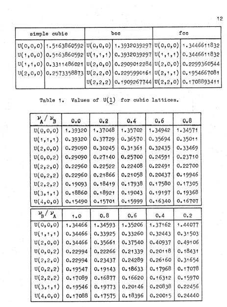
The evaluation of this integral is discussed in § 2 . 3 » and some values for the cubic and bet lattices are given in tables 1 and 2.

Random Walks on Defective Lattices.

For a defective lattice, we may express A ( 1 , 1 *) as

s i m p l e c u b i c b c c f e e

u ( o , o , o )

U ( 1 , 0 , 0 )

u ( M , o )

U ( 2 , 0 , 0 )

1 . 5 1 6 3 8 6 0 5 9 2

0 . 5 1 6 3 8 6 0 5 9 2

0 . 3 3 1 1 4 8 6 0 2 1

0 . 2 5 7 3 3 5 8 8 7 3

u ( 0 , 0 , 0 )

u( 1 , 1 , 1 )

U ( 2 , 0 , 0 )

U ( 2 , 2 , 0 )

U ( 2 , 2 , 2 )

1 . 3 9 3 2 0 3 9 2 9 7

0 . 3 9 3 2 0 3 9 2 9 7

O.29O9OI2284

0 . 2 2 9 5 9 9 0 1 6 1

0 . 1 9 0 9 2 6 7 7 4 4

u ( o , o , o )

u ( M , i )

U ( 2 , 0 , 0 )

U ( 2 , 1 , 1 )

U ( 2 , 2 , 0 )

1 . 3 4 4 6 6 1 I 8 32

0 . 3 4 4 6 6 1 1 8 3 2

0 . 2 2 9 9 3 6 0 5 4 4

0 . ^ 9 5 4 6 6 7 0 8 1

0 . 1 7 0 8 8 9 3 4 1 1

Table 1. Values of U(l) for cubic lattices.

V /

A' B 0 . 0 0 . 2 0 . 4 0 . 6 0 , 8

U ( 0 , 0 , 0 ) 1 . 3 9 3 2 0 1 . 3 7 0 4 8 1 . 3 5 7 0 2 1 . 3 4 9 4 2 1 . 3 4 5 7 1

u ( 1 , 1 , 1 ) 0 . 3 9 3 2 0 0 . 3 7 7 2 9 0 . 3 6 5 7 0 0 . 3 5 6 9 4 0 . 3 5 0 1 1

0 ( 2 , 0 , 0 ) 0 . 2 9 0 9 0 0 . 3 0 2 4 5 0 . 3 1 3 6 1 0 . 3 2 4 3 5 0 . 3 3 4 6 9

u ( 0 , 0 , 2 ) 0 . 2 9 0 9 0 0 . 2 7 1 4 0 0 . 2 5 7 0 0 _{0 . 2 4 5 9 1} 0 . 2 3 7 1 0

0 ( 2 , 2 , 0 ) 0 . 2 2 9 6 0 0 . 2 2 5 2 2 0 . 2 2 4 0 8 0 . 2 2 4 9 1 0 . 2 2 7 0 0

0 ( 0 , 2 , 2 ) 0 . 2 2 9 6 0 0 . 2 1 8 6 6 0 . 2 1 0 5 8 _{0 . 2 0 4 3 7} 0 . 1 9 9 4 6

0 ( 2 , 2 , 2 ) 0 . 1 9 0 9 3 0 . 1 8 4 1 9 0 . 1 7 9 3 8 0 . 1 7 5 8 0 0 . 1 7 3 0 5

0 ( 3 , 1 , 1 ) 0 . 1 8 8 6 0 0 . 1 8 9 2 1 0 . 1 9 0 4 3 0 . 1 9 1 9 7 O . 1 9 3 6 8

0 ( 4 , 0 , 0 ) Oo1 5 4 9 0 0 . 1 5 7 0 1 _{0 . 1 5 9 9 9} 0 . 1 6 3 4 0 0 . 1 6 7 0 7

V / V

B' A 1 . 0 0 . 8 O06 0 . 4 0 . 2

0 ( 0 , 0 , 0 ) 1 . 3 4 4 6 6 1 . 3 4 5 9 3 1 . 3 5 2 0 6 1 . 3 7 1 6 2 1 . 4 4 0 7 7

0 ( 1 , 1 , 1 ) 0 . 3 4 4 6 6 0 . 3 3 9 2 5 0 . 3 3 2 6 0 0 . 3 2 4 4 3 0 . 3 1 5 0 3

0 ( 2 , 0 , 0 ) 0 . 3 4 4 6 6 0 . 3 5 6 6 1 0 . 3 7 5 4 0 0 . 4 0 9 3 7 0 . 4 9 1 0 6

0 ( 0 , 0 , 2 ) 0 . 2 2 9 9 4 0 . 2 2 2 6 6 _{0 . 2 1 3 3 9} 0 . 2 0 1 1 8 _{0 . 1 8 4 3 1}

0 ( 2 , 2 , 0 ) 0 . 2 2 9 9 4 0 . 2 3 4 3 7 0 . 2 4 2 8 9 O. 2616O 0 . 3 ^ 6 5 4

0 ( 0 , 2 , 2 ) 0 . 1 9 5 4 7 0 . 1 9 1 4 3 0 . 1 8 6 3 3 0 . 1 7 9 6 8 0 . 1 7 0 7 8

0 ( 2 , 2 , 2 ) O . 1 7 0 8 9 0 . 1 6 8 7 7 0 . 1 6 6 2 0 O . 1 6 3 1 2 0 . 1 5 9 7 0

0 ( 3 , 1 , 1 ) 0 . 1 9 5 4 6 0 . 1 9 7 7 3 0 . 2 0 1 4 6 0 . 2 0 8 3 8 0 . 2 2 4 5 6

0 ( 4 , 0 , 0 ) 0 . 1 7 0 8 8 _{0 . 1 7 5 7 5} 0 . 1 8 3 9 6 0 . 2 0 0 1 5 0 . 2 4 4 4 0

the component p ( l - l ) being* that of the perfect lattice and q (l , 1 )

a perturbation. Suppose that the walker starts at 1 , so that

Pq (

1

8(1

1

1

Pt+1 (1) -

+ q(l ,l')]Pt(l’)

•

(16)

Summation of eqn. (16) from t *

0

o(i)

= 8(1 ,i0) +

o(i>i')o(i') ,

where

0(1) - ^ P t (1)

t=0

This set of equations can be solved in terms of U (l), which is the solution of

U(1) - ^ p ( i - i ’) u(i') = 8(1,0)

.

(17)

1* The equation

0(1) - ^ p ( l - l ’)0(l') » F(l)

(

18

)

1' has the solution

o(i) = y

(

-

,)

(

>)

,

(19)

~ L__. ~ ~

1' e+J

0(1) - y \ ( l - l ’)G(l’)

. 0(1) - ^ p(k)G(l-k)

1 ’

-= £ \ ( l - l ' )P(l') - ^ p ( k ) ^ U ( l - k -l')F(l’)

^F(l') U(l-l') - ^ p ( k ) U(l-l’-k)

1’

k

r

S(l- l1

t 0) (from eqn« (17))

LrnrnmJ) W ^ W **

F(l)

.

h'ow if we put

F(l) = 6(1 ,10) + £ \ ( l ,l')0(l')

1' in eqn. (l8) , then eqn.(1 9) becomes

0(1) « u(l-l0) + Y_

*i")G(i”)

1' 1"

(20)

If

q(l ,

1

• -• _ «

1 =

i-)

n' n

G(l) = U(l-10) + £ ^ U ( l - l lc)q(lk ,i) 0(f)

.

(21)

» I I . V

15

linear equations which can be solved for G(l^ ) > G(l^ ) , ... G(l^,) . Equation (21) can then be used to find G(l) for any lattice point 1 .

Calculation of Exchange Probabilities.

We can now express the exchange probabilities of §2.1 in terms of the function G(l) for suitably chosen defective lattices. To illustrate the method, the calculations will be carried out in full for the simple cubic lattice.

Let the sites around the origin in a simple cubic lattice be labeled as in fig. 3 > and suppose that initially the site is occupied by a vacancy and the site 0 by a tracer atom. The random-walk theory developed above will be applied the subsequent movement

movement of the vacancy. The theory deals with the probabilities of

jumps to particular s i t e s , and since we wish to find the

probabilities of certain exchanges with a particular tracer a t o m , we must ensure that the tracer atom remains on site 0 until the vacancy jumps to site 0 from site k^ or k^ . This is achieved by preventing

tracer-vacancy exchanges which take place entirely within the 0

plane, that is, by setting^i(0 , m ) = 0. The vacancies v/hich would have made jumps of this type must be distributed to the other

nearest-neighbour sites of each rcr site. This may be done by

increasing the appropriate jump probabilities to 1/5 , or, more

simply, by setting , rir) = 1/6. Once a vacancy has jumped to

site 0, it must be removed from further consideration, and therefore we set ^i(m , 0) = 0 and ^( k ^ , 0) = 0 .

Whenever the vacancy is on 3ite k the probability is 1/6

that it will jump to site 0 . Therefore 00

t =Q

z

m •

4 m

17

and similarly,

P _ “ * (?3)

Prom eqn. (15) we find that q(0, m. ) = q(m. , O) = q(k. , 0) = — 1/6 and q(riK , rrn) = 1/6 • On substituting these values into eqn. (21) we obtain

2 4

0 ( 1 ) = u d - k , ) - £ g(o) [ T U ( l - i c . ) + £ > ( 1 - ™ . )

1 = 1

(

)

♦ ifs(.)[o(i-»)-u(i.o)] .

o

L

j = 1

However, by symmetry, G(m ) =» G(m ) = G(m ) = G(m ) , and so eqn.(24) may be simplified to

2 4

G( 1) *= U ( l - k t) - £ g(0) 11(1-1^) + ^ U ( l - m . . ) i=1

4

G(®1) [

u(l“ 2j> - 4U(i>]

3=1

J=1

(25)

obtain

If we now substitute 0 and rn^ for 1 in eqn. (25) we

g(o) = U(1,0,0) - -g- 0(0) [6U(1,0,0)]

+ ^G(ra1) [4U (1,0,0) - 40(0,0,0)]] (26)

and

0(m,) = U(1,1,0) - £a(0)[U(0,0,0) + 4U(1,1,0) + U(2,0,0)]

U(0,0,0) = 1 + U(1,0,0)

and

U(1,0,0) - £u(0,0,0) + | u(1,1,0) + ^U(2,0,0) ,

and with the aid of these identities eqns. (26) and (27) can be simplified to

G(0)[U(0,0,0)] + G(m1 ) [ | ] - U(1,0,0)

and

0(0)[U1,0,0)] + o(

2

l)[i--iuO.o.o) + 1

u

(1,1,0)] = U(1,1,0)

.

On substituting values of U from table 1 into these equations, we obtain the solutions G(o) «= 0.2445397195 and

G(m ) = 0.2183541562 . ~1

From eqn. (25) »

c q p = u(0,0,0) - G(0)[U(1,0,0)] - G ( m ^ ) [ j U ( l , O tO) - jU(l,1,0)] (28) and

G(k2 ) . U(2,0,0) - G(0)[U(1,0,0)] - G C m p t l u O . O . O ) - |u(l,1,0)]. (29) The above values for G(0) and G ( m ) , together with eqns. (22) and (23), give P = 0.2271907074 and P = 0.0173490121 .

“f*

The calculations for the other lattices are very similar. The only additional difficulty which arises is that in some lattices

19

a s i n g l e s i t e . F o r e x a m p l e , f o r t h e b c c l a t t i c e we p u t Pq(i >1 >1 ) = Pq( 1 * 1 * — 1 ) = P 0 ( 1 , - 1 , 1 ) = Pq(1 >“ 1 j ”■ 1 ) = l / 4 , a nd t h e f i r s t t e r m on t h e r i g h t - h a n d s i d e o f e q n . ( 2 1 ) i s m o d i f i e d a c c o r d i n g l y .

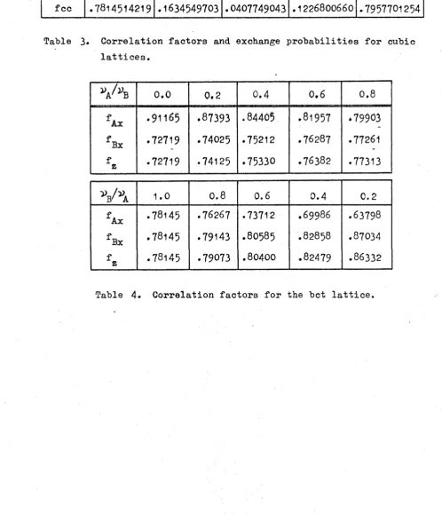
The p r o b a b i l i t i e s P+ a n d P a r e o f i n t e r e s t i n t h e t h e o r y

o f d i f f u s i o n i n a l l o y s . T h e i r v a l u e s f o r c u b i c l a t t i c e s a r e l i s t e d

i n t a b l e 3 , t o g e t h e r w i t h t h e c o r r e l a t i o n f a c t o r s . However, i f t h e

c o r r e l a t i o n f a c t o r s a l o n e a r e r e q u i r e d , t h e c a l c u l a t i o n i s

c o n s i d e r a b l y s i m p l i f i e d . B e c a u s e o f t h e i r s y m m e t r y , t h e l a t t i c e

d e f e c t s c o n t r i b u t e e q u a l a m o u n t s t o P and P ( c f . e q n s . ( 2 8 ) an d

( 2 9 ) ) . T h u s , t o f i n d Q( = P - P ) , t h e r e i s no n e e d t o i n t r o d u c e

t h e d e f e c t s . E q u a t i o n ( 2 1 ) t h e n becomes

G ( l ) = U ( l - 1 0 ) .

The r e s u l t i n g e x p r e s s i o n s f o r Q c a n be w r i t t e n a s i n t e g r a l s w i t h t h e

a i d o f c q n . ( l 4 ) . F o r t h e s i m p l e c u b i c l a t t i c e , we h a v e

Q -

£ [ u ( o , o , o ) - u ( 2 , o ; o ) ]

(1 - c o s 2u ) du dv dw

rr tr rr

0 0 0

1 - — ( C O S U + C O3 V + c o s w )

F o r t h e b c c l a t t i c e ,

( 3 0 )

Q = ^ [ U ( 0 , 0 , 0 ) + - U ( 2 , 0 , 0 ) - U ( 2 , 2 , 0 ) - U ( 2 , 2 , 2 ) ]

tt rr rr

0 _+ CQS 8U ~ c o s 2 v - c o s 2u co s 2v C032w) du dvdw

1 - c o s u c o s V c o s w

For the fee lattice,

Q = ~ [ U ( 0 , 0 , 0 ) + 2U(1,1,0) - 2U(2,1,1) - U(2,2,0)j

TT Tf Tf

1 2tT'

(1 + 2 cos u eos v ~ 2 eos 2u co3 v cos w - cog 2u cos 2v)du dv dw

' 0 0 0

For the bet lattice,

4

1 - — ( cos u COS V + COS V cos w + cos w cos u)

Q,

U(0,0,0) + 2U(2,0,0)+ U(2,2,0)- U(0,0,2)- 2U(0,2,2)- U(2,2,2)

rr tt t f

1

3

(1 + 2 cos 2u+ cos 2u cos 2v - cos 2w

- 2 cos 2v cos 2w - cos 2u cos 2v cos 2w) du dv dw 1 - M u )

0 0 0

u(0,o,o) - u(4,o,o)

1

tt tt tt

J U c 0 0 0

V s

TT Tt Tf

0 0 0

(1 - cos 4u) du dv dw 1 - "X (u)

U(1,1,1) - U(3,1,1)

( cos u - cos 3u) cos v cos w du dv dv/ 1 - X (u)

BB ^ B

U(0,0,0) + U(0,0,2) - U(2,2,0) - U(2,2,2)

Tt IT Tf

u

(1 -f cos 2w - cos 2u cos 2v - cos 2u cos 2v cos 2\v) du dvdw 1 - X (u)

21

where ^ =

v j

^

The values of the correlation factors for the hct lattice are shown in table 4 and fig. 4.

§2.3 > Evaluation of Integrals.

The first step in the evaluation of the integral in eqn. (14) for

a particular lattice

lattice point

For the simple cubic lattice, eqn. (1 1) becomes ^(u ) = £ [ei(UfV,w).(T,0,0) + ei(u,v,w).(-t,0,0)

+ 0i(u,v,w).(0,1,0) + ei(u,v,w).(0,-1,0) + 0i(u »v,w). (0,0,1) + Qi(u, v, w ) . (0,0,-1 ) -j

1 / :

- Z (e + e

-iu -iv -iw

+ e + e** + e + e )

~ (cosu + cos v + cosw )

For the bcc lattice,

7v(U ) - £ [ei(u+v+w) + ei(u+v-w) + ei(u-v+w) + ei(u-v-w) i(-u+v+w) i(-u+v-w) i(-u-v+w) i(-u-v-w)

^ 0 + 6 + 0 "f 0

1 / iu - i u w iv - i v w iw , - i w x ■ g (e + e ;(e + e )(e + e

)

L a t t i c e f P

+ P_ Q _{p ß}

s c

b c c

f e e

.6 ^ 3 1 0 8 8 3 8 8

. 7 2 7 1 9 4 1 4 0 1

. 7 8 1 4 5 1 4 2 1 9

. 2 2 7 1 9 0 7 0 7 4

. 2 2 0 0 8 8 7 0 5 0

. 1 6 3 4 5 4 9 7 0 3

. 0 1 7 34 90 12 1

. 0 6 2 1 4 1 2 8 4 0

. 0 4 0 7 7 4 9 0 4 3

.2 0 9 8 4 1 6 9 5 3

.1 5 7 9 4 7 4 2 0 9

.1 2 2 6 8 0 0 6 6 0

. 7 5 5 4 6 0 2 8 0 4

. 7 1 7 7 7 0 0 1 1 0

. 7 9 5 7 7 0 1 2 5 4

T a b le 3* C o r r e l a t i o n f a c t o r s and e xc h an g e p r o b a b i l i t i e s f o r c u b i c

l a t t i c e s .

b A 0 . 0 0 . 2 0 . 4 0 . 6 0 . 8

f Ax . 9 1 1 6 5 .8 7 3 9 3 . 8 4 4 0 5 .8 1 9 5 7 .7 9 9 0 3

f Bx . 7 2 7 1 9 . 7 4 0 2 5 . 7 5 2 1 2 . 7 6 2 8 7 .77261

f

z . 7 2 7 1 9 . 7 4 1 2 5 . 7 5 3 3 0 . 7 6 3 8 2 .7 7 3 1 3

V » A 1 . 0 0 . 8 0 . 6 0 . 4 C. 2

f Ax . 7 8 1 4 5 .7 6 2 6 7 . 7 3 7 1 2 .6 9 9 8 6 .6 3 7 9 8

f Bx . 7 8 1 4 5 . 7 9 1 4 3 . 8 0 5 8 5 .8 2 8 5 8 .8 7 0 3 4

f

z . 7 8 1 4 5 . 7 9 0 7 3 . 8 0 4 0 0 . 8 2 4 7 9 . 8 6 3 3 2

23

for the fee lattice,

X (u) = ^ ( C O S U C O S V + C O S V C 0 9 w + cos w c o s u) .

l‘or the bet lattice,

"X (u) = 2yu^ (cos + cos 2v) + 8jx^ cos u cos v cos w ,

where » vA /(4 + 8i)ß ) and /xQ = ^ / ( 4 VA + 8 Vß ) .

If 1 * (1. , 1 0 , 1-, ), eqn. (14) becomes

~ 1 c j

i t it ,rr

U(l)

(2ir)

’’ i(l u + 1 v + 1 w)

e v 1 2 3 d u d v dw

1 - X (u)

-TT -TT -TT

W J

( cosl^w + i sinl^w)

-TT

Ü

-TT

(cosl^v + i sinl^v)

TT

n

u

- T T

( cos l ^ u + i sin l^u) du dv dw

1 - X (u) rr TT tr

0 0 0

cos 1 ^u cos l^v cos l^w du dv dw

1 - X (u)

(31)

The numerical evaluation of the integrals obtained from eqn. (31) is not completely straightforward, as the integrands all

have at least one discontinuity in the integration volume. The

simplest case is the simple cubic lattice, where we have

TT IT TT

u(i) - Jj

TT .

° cos 1 ^u cos l^v cos 1 ^w cu dv dv/

0 0 0

25

in which the integrand has an infinite discontinuity at the origin. The integration volume is a cube with edge tt . If we delete from this volume the cube of edge tt/2 containing the origin, the integration over the remaining volume can be carried out

numerically. From the cube of edge rr/ 2 we now delete a cube of edge tt/ 4 , and so on. Y/e thus obtain a series of integrals which converges to U(l) . Only the first few terms of the series need be evaluated, because the series tends to a geometric series with common ratio — .

F o r the bee, f e e a n d b e t l a ttices, the i n t e g r a n d in eqn.

(3l) has more than one discontinuity in the integration volume. However, in each case

it

The values of U(l) should obey eqn. (17) > which therefore provides a check of the accuracy of the numerical integration.

The same methods can be used to avoid the discontinuities in the integrands of eqn. (30) and the equations following it.

§ 2.4.__Conclusions.

A general method for calculating jump probabilities for random walks on lattices has been developed. The theory has been applied to the calculation of certain tracer-vacancy exchange probabilities, which are related to correlation factors for diffusion by the vacancy mechanism. Correlation factors for

27

§3. CORRELATION FACTORS FOR DIFFUSION IN UNORDERED BINARY ALLOYS.

The diffusion of vacancies in pure materials is uncorrelated, hut Manning (1967a) has shown that in alloys the diffusion of vacancies is usually correlated. In this section, some improvements are made to Manning's theory of diffusion by the vacancy mechanism in unordered binary alloys (Manning I967a>b). These improvements lead to qualitatively different results in certain limiting cases.

We consider a homogeneous unordered binary alloy of cubic structure, containing mole fractions N^ and N^ of atomic species A and B. Fluctuations in average local composition are ignored, and it is assumed that vacancies are not bound to any particular atoms. Vacancy jumps are of two kinds : exchange with a neighbouring A atom or exchange with a neighbouring B atom. The corresponding jump frequencies are denoted by w^ and , and are assumed to be independent of the identities of the surrounding atoms. These assumptions are best satisfied in non-dilute alloys. It is convenient to choose the labels A and B such that w^ ^ w^ .

Since diffusion in cubic crystals is isotropic, all sets of axes are principal. Let us choose an x axis perpendicular to the (100) planes, and let n be the number of ways in which an atom (or

a

vacancy) can jump to an adjacent (U)0) plane. In the simple cubic lattice n = 1 , and in the bcc and fee lattices n = 4 .

a a

respectively. (Note that crT is measured in the sense of the T

original tracer jump and cr in the sense of the original vacancy

\ T

jump.) The corresponding correlation factors f^ and f are given by

and

1 + 2ov

1 + 2 a

(32)

(33)

Equation (

3

D* = n N wm d? f_

T a v T T (

34

for diffusion of atoms and

n N w d^ fA + n N_. w u d2 fB

a A A v a B B v (

35

for diffusion of vacancies, where d is the lattice spacing and N is the mole fraction of vacancies.

A B

In addition to the partial correlation factors f and f"

v v

we can define an average correlation factor f by the equation

n W d f

a v (36)

where W is the average vacancy jump frequency, given by

W “ \ WA + V

•

* This notation has been chosen to agree v/ith Manning's, although

T

v