L ea rn in g , an d S w itc h in g
C o n tro llers
Laurence S. Ir licht
B.Sc. Hons. (Melb), Dip. Ed. (Melb)
A thesis submitted for the degree of Doctor of Philosophy of the Australian National University
Department of Systems Engineering
Research School of Physical Sciences and Engineering,
Co-operative Research Centre for Robust and Adaptive Systems
The Australian National University
A c k n o w le d g e m e n ts
I would like to thank the students and staff of the Systems Engineering Department for providing a stimulating environment in which to work. More specifically, I thank my supervisor, John Moore, for having the patience to guide me in the initial stages of my course, and the wisdom to allow my independence to grow toward the end. John taught me a lot about engineering, and also a lot about living.
I would also like to thank Iven Mareels for helping me to develop my ideas, for a shared enthusiasm to research, and for many fruitful discussions on matters well beyond those contained in this thesis.
This acknowledgement would not be complete without reference to the many friends who have been there for me during the last 3 years, especially Perry Black- more, and also Brian Ewert, David Ekselman, and Simon Inglis.
The work presented in this thesis is the result of original research done by myself in collaboration with others in the time I have been enrolled in the Department of Systems Engineering as a Doctor of Philosophy student. It has not been submitted for any other degree or award in any other university or educational institution. Much of it has been published or accepted for publication in refereed journals and conference proceedings, [28, 30, 33, 43], or submitted for publication [31]. At times, I worked on developing ideas by supervisors, and at other times they gave me help on my own ideas. Certainly, I identify very closely with 100% of the thesis content, and yet my supervisors probably also identify closely with large portions of the thesis as well. The specific contributions I particularly identify with are summarized as follows:
• The nonlinear Q, S stabilization results of Chapter 2 were carried out jointly by myself and Prof. Moore. I also developed the simulation section by streamlining the original code, and extending it to cope with various disturbances, repeated trajec tories and unmodelled dynamics.
• The idea of utilising a functional-learning Q scheme was Prof. Moore’s. We worked together on the implementation issues, and I extended the developed methods to the vector case, created the programs used to implement functional learning the ory, spliced them into the adaptive-Q program and designed and implemented the simulations.
• The problem of extending time-varying factorization results to a nonlinear context was suggested by Prof. Moore. The key observations that state dependent systems could in the right factorization case, and in inversion and cascade, behave like linear time-varying systems are mine. Prof. Moore suggested the augmentation approach, and I designed the augmentations, and formulated and proved the limitations of this approach. Prof. Moore and I worked together to incorporate the known non-linear stability results, and I designed and implemented the simulations.
• Prof. Moore suggested the idea of using switched controllers for resonance suppres sion, and initial discussions as to im plem entation were held between Prof. Moore, Dr. M areels, and myself. I carried out the rest of the work alm ost independently.
In this thesis we investigate new methods of analysis, design, and application of adap tive, learning, and switched controllers. We view these controllers as examples of state dependent systems, i.e. systems with a state space description in matrix form with the system matrices being functions of the state of the system. This viewpoint encourages their application to the robust control of state-dependent, and uncertain plants, and leads to new stability results.
In the first part of the thesis, we build upon known linear and nonlinear factorization theory, and the Youla-Kucera parametrization, to study the blending of off-line designed optimal controllers with adaptive and learning controllers. The feedback controller is designed for a state dependent system, namely the actual plant linearized about an opti mal trajectory. The inclusion of this controller results in robustness enhancement, with performance enhancement in the non-nominal case.
Motivated by this work, a more complete factorization theory for state dependent systems is developed. Stabilization results are recalled which require such factorizations to achieve the identification of classes of all stable pairs of state-dependent plants and controllers. These classes are parametrised by the so called {Q,5} parametrisation.
Further stability results are then generated for linear time-varying (periodic) systems. These results, which bound the difference between the trajectories of these systems and the trajectory of stable “averaged” linear time-invariant systems, provide results which are shown to achieve dramatic reduction in controller order, and effective implementation of hybrid control.
Finally, resonance suppression via “switched” controllers is proposed. It appears that such systems, although very effective, are beyond the scope of present analysis techniques. In this thesis they are put forward as an area for future research with preliminary simu lation studies. Key arguments are provided to illustrate the importance of such switched systems, which are themselves an example of state-dependent, adaptive controllers. It is
Acknowledgements... i
Statement of Originality... ii
A b stra c t iv 1 In tr o d u ctio n 1 1.1 General B ac k g ro u n d ... 1
1.2 State-Dependent S y s te m s ... 2
1.3 Analysis T e c h n iq u e s ... 3
1.4 A pplications... 5
1.5 Outline of T h e s is ... 6
2 R o b u st N o n lin e a r C ontrol - A d a p tiv e Q 10 2.1 Introduction... 10
2.2 Self-Tuning Optimal Nonlinear C ontrol... 12
2.3 Convergence Properties ... 20
2.4 S im u latio n s... 29
2.5 C onclusions... 34
3 R o b u st N o n lin ea r C ontrol - S ta te D ep en d e n t Q 36 3.1 Introduction... 36
3.2 Least Squares Functional L e a rn in g ... 38
3.3 Learning-Q Controller Scheme ... 41
3.4 Simulation Results ... 43
3.4.1 Selection of Algorithm P a ra m e te rs ... 45
3.4.2 Results ... 46
3.5 Conclusion ... 49
4 C o p r im e F a c to r iz a tio n s o f S ta te D e p e n d e n t S y s te m s 50
4.1 Introduction... 50
4.2 Nonlinear Factorizations... 52
4.3 Systems with output dependent nonlinearities... 65
4.4 Augmented Systems Factorizations... 73
4.5 Simulation R e s u lts ... 89
4.6 Conclusion ... 92
5 T im e D e p e n d e n t S w itc h in g C o n tr o lle r D e s ig n 93 5.1 Introduction... 93
5.2 An averaging analysis of periodic s y s te m s ... 96
5.2.1 Introduction ... 96
5.2.2 Definitions ... 96
5.2.3 P ro p o sitio n ... 98
5.2.4 Fundamental Averaging Result... 98
5.2.5 Explicit Averaging Results for Linear Systems ... 99
5.3 Controller Sim plification... 105
5.4 A Case S t u d y ...110
5.5 Discrete-time control of a continuous-time p la n t...114
5.6 Conclusion ... 117
6 S t a te D e p e n d e n t S w itc h in g C o n tr o lle r D e s ig n 119 6.1 Introduction... 119
6.2 Switched Controller A lgorithm s... 122
6.2.1 Introduction ... 122
6.2.2 Aims of Controller D e sig n ... 123
6.2.3 Description of Controller D e s i g n ... 124
6.2.4 Switching A lg o rith m ...124
6.2.5 Parameters of switching system: ... 126
6.3 Simulation R e s u lts ... 127
6.3.1 Example of Stabilization via Switching and M ix in g ... 127
6.3.2 Switching control of a stable P l a n t ... 129
6.4 Conclusion ... 131
7 C o n c lu s io n 132
7.2.1 New Theoretical R e su lts...133 7.2.2 New Algorithms ... 133 7.3 Areas For Further R e se a rc h ... 134
B ib lio g r a p h y 136
A 143
A. l Proof of Lemma 3.1 of Chapter 3 ... 143
B 144
B. l Preliminary Results of Chapter 5 ... 144
L ist o f F ig u res
2-1 The Augmented Plant A rra n g e m e n t... 14
2-2 The Linearized Augmented P l a n t ... 15
2-3 Class of all Stabilizing Controllers for AGo ... 16
2-4 Class of all Stabilizing Controllers... 17
2-5 Adaptive Q for Disturbance Response M in im iz atio n ... 20
2-6 Two degree-of-freedom adaptive-Q schem e... 21
2-7 The Least Squares Adaptive-Q Arrangement ... 21
2-8 Model Reference Adaptive Control Special Case...22
2-9 The feedback system (A G (5), K(Q)}... 30
2-10 The feedback system {Q ,S}... 31
2- 11 Open Loop and LQG/LTR/Adaptive-Q T raje c to rie s... 33
3- 1 Two-degree-of-freedom learning-Q scheme (A-D converters not shown) . . . 43
3-2 Five Optimal Regulation Trajectories in r il)l2 space... 44
3- 3 Comparison of Error surfaces learnt for various grid cases... 48
4- 1 Cascade of System P2 and System P i ... 54
4-2 Equivalent loops for the pair {G(x), i f (x)}... 58
4-3 The system G s(x0) ... 62
4-4 The Feedback System {Gy, K y} ... 65
4-5 The Feedback System { NyM ~ l ,UyV ~ 1} ... 66
4-6 The Feedback System {Gy, i f * } ... 66
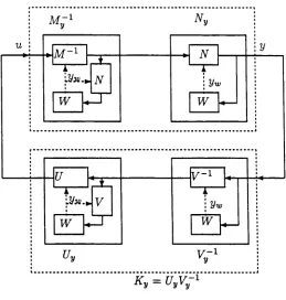
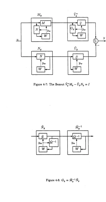
4-7 The Bezout V*My — (jyN y — I ... 67
4-8 Gy = M ~ l Ny ... 67
4-9 The Bezout M*V* - NyUy* = I ... 68
4-10 KJ = U;Vy— 1 ... 68
4-11 The Bezout V x M y — Üy Ny = I ... 70
4-14 The system {^(xo),/C(xq)} ... 75
4-15 The block [AT(xo) Ar,(xo)]/ ... 76
4-16 The feedback system (£(xo),/C(xo)} in factor form... 77
4-17 The feedback system (£(xo), /C(xo)} in simplified form... 78
4-18 The Bezout V(xo)A4(xo) — Ü(xo) N(xq) = I ... 79
4-19 The class Kq ... 81
4-20 The class Kq t ... 81
4-21 The Bezout M. R — Af S = [7 0 ] ' ... 82
4-22 The class £ s ( x o ) ... 84
4-23 The system {^5(xo),/Cgr (xo)} ... 85
4-24 The system {5(xo, xo)> Q r ( ^ o ) } ... 85
4-25 The matrix blocks A - D for Plants 1-4... 89
4-26 The controller and augmented plant states at each time instant... 90
4- 27 The Q-parametrised controller and nominal plant states at each time instant . 91 5- 1 The feedback system {G , K}... 106
5-2 Comparison of x(t),y(t), z(t) ...I l l 5-3 Comparison of plant trajectories with the full, and first order controllers. . 113
5- 4 Sampled hold system {h^ G , K }...116
6- 1 Switched control S y ste m ... 122
C h a p te r 1
I n tr o d u c tio n
1.1
G e n e r a l B a c k g r o u n d
Feedback controllers are often designed to operate within certain hard constraints such as total energy utilised, maximal allowed acceleration, etc. Beyond this, the controller may be optimised for one, or a combination of three objectives:
1. Robustness to Plant Uncertainty:
The actual plant may not be identical to the nominal one. Usually, it is assumed that the actual plant will be within some uncertainty region of the nominal. The controller must be designed to stabilize all plants within this region.
2. Robustness to Noise:
The controller must stabilize the plants in the uncertainty region in the presence of some form of stochastic noise.
3. Performance Objective:
Given a specific controller, plant and noise environment, the quality of control may be measured via the application of a cost function. This function quantifies the performance by comparing the state and output of the plant and utilised control energy with desired values. The controller must stabilize the plants within the uncertainty region in some economical manner with respect to the cost function. During the operation of a plant, measured signals become available which can permit restriction of plant uncertainty. Since the knowledge of the plant or of the closed loop is improving, new or modified controllers may be designed, perhaps on-line, to incorporate this knowledge, and therefore provide improved performance and robustness. To this end,
for our purposes, we define two classes of controllers which are designed to make use of the increasing information.
Adaptive controllers are those designed to modify their dynamics based on measured signals. This is generally done in one of two ways. Direct adaptive control adjusts parame ters of a fixed controller to achieve performance objectives. For example, Model Reference Adaptive Controllers modify their behaviour to attempt to force the closed loop system to approximate a given model. Alternately, indirect adaptive controllers estimate the plant parameters, and then modify the controller according to some design method using plant model estimators.
Learning controllers are also adaptive, but have the ability to more effectively learn from their experience. To achieve this, they store large amounts of data, such as input- output maps, and use this to generate behavioural information. They differ from standard adaptive controllers both in their ability to choose the data they work with, and also in their capacity to generate and extrapolate knowledge of the system. This added complexity results in a sophisticated adaptive controller which intelligently controls its own adaptation process.
Another very common type of controller which modifies its behaviour on-line, is a gain scheduled or switched controller. More generally this may be structured as an adaptive or learning system. The switched controller consists of a bank of (usually) a-priori designed controllers, and a switching rule which decides which controller is to be active at a given time. One appeal of switched controllers is their stability for plants with known discon tinuities, for when the trajectory of the plant crosses a discontinuity, a more appropriate controller can be switched in without the losses incurred during standard adaptation.
Adaptive, learning, and switching controllers have found much application to areas such as aircraft control, process control, and robot manipulation, etc. However their inherent nonlinearity makes their analysis non-trivial, and in some cases even intractable. How then are they to be analysed?
1.2
S t a t e - D e p e n d e n t S y s t e m s
1.3 Introduction 3
x = A(x)x + B{x)u, x(0) = xo (1.2.1)
y = C(x)x + D(x)u
Here A(.) ,£ ( .), C(.), D(.) are the state-dependent matrix blocks, x is the state, u is the input and y is the output of the system.
Linear time invariant and time varying systems are two well known members of the class of state-dependent systems. Also, many processes not well modelled as linear systems may be more accurately modelled as state-dependent systems. Consider for instance the problem of controlling an aeroplane. Clearly, a full state vector will include such variables as the altitude and velocity. These variables affect the aeroplane’s dynamics. Other variables such as temperature and pressure, which directly affect the performance but are only indirectly affected by the controller, may be viewed in this approximation either as uncontrollable states, time-varying parameters, or stochastic disturbances.
Adaptive controllers may be viewed as state-dependent systems, since for these systems the feedback control gain is a function of system output [53]. In a similar way, many learning and switched controllers, such as those developed in this thesis, can be described by (1.2.1). The implication of this viewpoint forms an important stimulus toward to the applications and techniques developed.
1 .3
A n a ly s is T e c h n iq u e s
The stability results of this thesis are based on Matrix Fraction system descriptions, Co prime Factorizations [72], and Averaging Theory [57].
Previous work in factorization theory has added much to the knowledge and design of robust linear control systems and permits a very convenient characterisation of the class of all stabilizing controllers for a plant or the dual class of all plants stabilized by a given controller. This work is of particular interest for adaptive and learning control as it provides results guaranteeing robustness of a parametrised controller/plant system. It can be applied so as to restrict the adaptation to a class of stable feedback systems.
In some cases, techniques such as linearization about a fixed point and feedback lin earization, etc. [59], have been applied to minimise the apparent nonlinearity of a system and hence lead to greater application of linear theory. In general, the more non-linear the system, the less theory there is to help. The result is that many of these methods either only work for certain restricted classes and operating regions, or lose the full power of the linear techniques.
A further analysis technique applied here is that of averaging theory which demon strates how the trajectories of an intractable system, such as a time-varying system, are bounded with respect to those of an analytically tractable time-averaged system. This powerful analysis technique is finding increasing application to control theory, (see for instance [1] and its references). Here it is applied in reverse, namely to the identification of the trajectories of a simple system with those of a class of higher order systems. The added degree of freedom inherent within this class is utilised to improve computational effort and robustness.
The major objective of the analysis techniques developed here is to aid in the pre diction, and consequently the design of stable adaptive, learning and switched systems. Our study restricts to a class of nonlinear systems close to linear in some sense, but with immediate application to feedback control. The aim is not to develop a full theory for the analysis of nonlinear systems, but to explore some new areas which in may in turn enhance existing theory. To this end we investigate factorization and stability theory of two key classes of nonlinear systems, and the asymptotic behaviour of one class of linear time varying systems.
The analysis techniques developed here include:
1. The nonlinear Q , S stabilization results of Chapter 2. These may be applied to generate the class of all (nonlinear) stabilizing controllers for (nonlinear) systems, both expressed as a linear kernel perturbed by a nonlinear system, one form of the so-called Q , S formulism. Many controllers including those developed in Chapters 2, 3 and 6 may be effectively described in this way. In some cases however, the entire complexity will remain within the Q , S subsystem. Thus the theory has gen eral application, but the simplification provided will be dependent on the specific application.
differ-1.4 Introduction 5
ential boundedness of the factors permits a characterisation of all plants stabilized by a given controller, and the dual. In comparison with the results of Chapter 2, there is here a more restricted class of systems, but the increased simplification is considerable.
3. The averaging techniques of Chapter 5 allow analysis of switched systems in the case of fast periodic switching. These techniques lead to certain implementation advantages with regard to computational effort. They also give some insight into the asymptotic behaviour of the more complicated state-dependent switching schemes of Chapter 6. As such they are intended as one starting point for a more complete theory of state-dependent switched systems.
1 .4
A p p lic a tio n s
The first application we investigate is the robustness enhancement of open-loop optimal controllers for nonlinear systems. A major problem with many standard open-loop designs is that they are less robust than alternative closed loop techniques. However, for many nonlinear systems, the calculation or implementation of closed loop optimal controllers may be impractical. A standard method of adding robustness properties to an open-loop optimal control system involves adding feedback to the controlled system. To achieve this, the system is first linearized about the optimal trajectory. Subsequently, a feedback controller is designed to stabilize the linearized system by forcing the actual trajectory closer to the optimal one.
Any system derived from linearization about a non-stationary trajectory will be time- varying. Furthermore, the actual state of the nonlinear system will be affected by ex ogenous signals. These factors motivate the use of an adaptive controller. Here this is achieved via application of a robust and adaptive Q parametrization control technique. The Q parameter of the proposed scheme is an adaptive filter, and the adaptation task is to adapt the Q filter toward one which encourages close tracking of the optimal trajectory despite disturbances, unmodelled dynamics, etc.
A natural extension to the parameter tuning of the adaptive-Q methods is to what we term Learning-Q methods. In this case, the optimal Q filter parameters are identified as functions of the plant’s state. Consequently, the tuning procedure involves the learning of these relations. An investigation of such learning-Q systems forms the second application.
controller implementation. These controllers may be applied to achieve effective model- order reduction and hybrid control. Theoretical results and simulation studies show that the performance loss, as compared to the standard high-order continuous-time implemen tations, vanishes as the speed of switching increases.
The final application of this thesis is to resonance suppression via state-dependent switched controllers. Low order switched controllers are shown to effectively control high order uncertain plants in the presence of noise. Although complete analytical results have not been forthcoming, simulation studies and certain theoretically based observations indicate that the switched controller design is indeed a useful one for such control problems.
1.5
O u tlin e o f T hesis
The thesis is divided into seven chapters, with Chapters 2 to 6 based on referenced pa pers. The content of each chapter is largely self contained. Together they present new techniques for the analysis and application of certain state dependent control systems. More specifically, the areas covered by each chapter are :
Introduction
Chapter 3 describes one approach to the application of functional learning tech niques to the problem studied in Chapter 2, namely to assist in achieving near optimal control of nonlinear systems in the presence of disturbances and/or unmod elled dynamics. We still work with the standard approach to achieving robustness of open loop optimal control of nonlinear systems; that of applying feedback control based on plant linearization and application of linear quadratic control methods. In Chapter 2, we show that such methods can be enhanced by augmenting with adaptive loops, achieving what is termed adaptive-Q control. Here, instead of the adaptive-Q filter being a linear system with coefficients adjusted by a least squares law, the filter’s coefficients are functionally dependent on a subset of the optimal states associated with a nominal plant. The functional representation is updated by a least squares law in the case that ‘measurements’ are linear in the function’s unknown parameters, as when the function is represented by a sum of bisigmoids in the function input variable space. Such algorithms, and their convergence proper ties, have been previously studied in an identification context.
A simulation study of the optimal quadratic regulation of the nonlinear 2-state Van der Pol equations is used to demonstrate improved performance in the presence of disturbances, with both the nominal plant and one perturbed by unmodelled dy namics. The approach could well have application in areas such as aircraft control or robot control where gain schedules are learnt on line. This work is also reported in [33].
of an arbitrary stable system (parameter). Plant uncertainties, including unknown initial conditions are modelled by means of a Yula-Kucera type parametrization ap proach developed for nonlinear systems. Certain robust stabilization results are also shown, and simulations demonstrate the regulation of nonlinear plants using the techniques developed. All the results are presented in such a way that specialization to the case of linear systems is immediate. This work is also reported in [43, 44]. • Chapter 5 details the analysis and simulation of the class of switched systems with the
switching function a periodic function of time. We first demonstrate via averaging theory, an approach whereby any stable linear system can be approximated by a simple periodic-structure system.
Next is proposed the control of continuous-time, linear, time-invariant plants via a periodic structure control scheme with a rationale based in averaging analysis. It is established that for continuous-time minimal plants it is possible to design periodic-structure stabilizing first-order controllers which asymptotically approach the performance of an n th order stabilizing time-invariant controller, such as an op timal (LQG) controller, in the limit as the switching rate increases. The proposed controllers suffer only a small loss of performance compared with the n th order con troller, are attractive from a computational point of view, and may be implemented in either discrete or continuous time. Simulation results are shown which demon strate the efficacy of the proposed controllers. This work is also reported in [31, 32]. • Chapter 6 then extends the studies of Chapter 5 to the more general case of the
1.5 Introduction 9
R o b u st N on lin ear C ontrol
-A d a p tiv e
Q
2.1
I n t r o d u c t io n
Optimal nonlinear deterministic control methods are considered very elegant in theory, but lack robustness in practise. In the optimal control approach, a mathematical model of the process is first formulated based on the fundamental laws in operation or via identification techniques. Next, a performance index is derived which reflects the various cost factors associated with the implementation of any control signal. Then, off-line calculations lead to an optimal control law u* via one of the various methods of optimal control. In theory then, applying such a control law to the physical process should result in optimal performance. However, the process is rarely modelled accurately, and frequently is subject to stochastic disturbances. Consequently, the application of the “optimal” control signal u* results in poor performance, in th at the process output y differs from y*, the output of the idealized process model.
One approach to achieve improved performance could be to include robustness mea sures in the cost function, so that for plants “near” the nominal model and “small” dis turbances poor performance is avoided. This approach turns out to be difficult to develop in practise.
A standard approach to enhance open-loop optimal control performance is to measure on-line the difference between the ideal optimal process output trajectory y* and the actual process output y. This difference signal, 8y, depends on the difference, <$u, between the optimal control u* for the nominal model and any actual control signal u applied.
2.1 Robust Nonlinear Control - Adaptive Q 11
For nominal plants with suitably smooth nonlinearities, and small differences bu, by, a linearization of the process allows an approximate linear dynamic model for relating by
to bu. With this model, optimal linear regulator theory can be applied to calculate bu in terms of by which is measurable, so as to regulate by to zero. Indeed, the linearization can extend to yield an associated quadratic performance index consistent with the original nonlinear index so that linear optimal control (LQG) theory can be applied to achieve optimal regulation of by under the linearization assumptions. Robust regulator designs based on optimal theory, perhaps via loop-transmission recovery (LTR), could be expected to lead to performance improvement over a wider range of perturbations on the nominal plant model.
Even with the application of linearization and feedback regulation to enhance optimal control strategies, there can still be problems with external disturbances and modelling errors. The linearization itself may be a poor approximation when there are large pertur bations from the optimal trajectory.
2.2
S e if-T u n in g O p tim a l N o n lin e a r C o n tr o l
Signal Model/Optimal Control Plant Performance Index and Linearization
Consider a generalized nominal plant model :
Go : x = /( x ,u ) , y = h{ x, u) , x(0) = xq (2.2.1)
and some performance index over the time interval [0, T]
/ = [ l{x,u)dt (2.2.2)
Jo
with associated optimal control u*, state x*, and output y*. Consider also a linearized version of the above plant model, denoted AGo(x*);
AGo(x*) : d(6x)/dt = A6x + B6u
6y = C8x 4- D8u[= AGo(x*)6uj
where 6x(0) = 0 and A, B, C, D = §£|x _
The following shorthand notation proves useful subsequently,
(2.2.3)
AG0(x*) A B
C D
(2.2.4)
With AG the operator denoting the actual system with input 5u = u — u*, state 6x = x*
and output 6y = y — y*, then AGo denotes a linearized version of AG.
Let us associate with the linearized model a quadratic performance index penalising departures 6y and 6u away from the optimal trajectory.
where,
AI
f
(2.2.5)6y Q c S c
2
» L = , Q c >, Q c - o S c R ; l S c>0 , 0 ( 2 . 2 . 6 )
6u
i
---
R cHere e is interpreted as a disturbance response which we seek to minimise in an Li
2.2 Robust Nonlinear Control - Adaptive Q 13
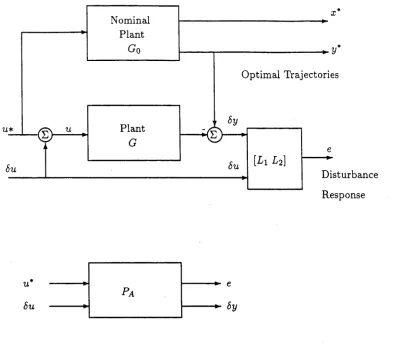
We assume that u*,x*,y* are known a priori, but that when applied to an actual plant G, which includes unmodelled disturbances and/or dynamics, there are departures from the optimal trajectories. With departures by = y — y* measured on-line, a standard approach is to apply control adjustments bu = u — u* to the optimal control by means of feedback control to minimise (2.2.5). Thus for the augmented plant arrangement, denoted P^, and depicted in Figure 2-1, let us consider a linear feedback regulator. We base such a design on the linearized situation depicted in Figure 2-2 where the linearized nominal plant, denoted Pq, is given from
Po = * P\2
* P22
(2.2.7)
P n = L AGo(x*) I
P22 = AGo(x*) (2.2.8)
The terms P u , P21 are not of interest for subsequent analysis.
Feedback Regulator for Performance Enhancement The regulator of the linearized model Po is
K0{x*) : d(bx)/dt = Abx + Bbu - Hr ,<5x(0)=0
r = by — Cbx — D6u
du = F6x [= K 0{xm)6y] (2.2.9)
Here r is the estimator residual, <5x is the estimate of 6x and H and F are time-varying ma trices formed, perhaps via standard LQG/LTR theory [2], so that under uniform stability of A,B and uniform detectability of A,C the following systems are exponentially stable.
M + BF)£f , £h — (-^ + HC)£h (2.2.10)
Actually, the important aspect of the LQG design for our purposes is that under the relevant uniform stabilizability and uniform detectability assumptions, the (time-varying) gains H, F exist, and are given from the solution of two Riccatti equations (with no finite escape time). Moreover, for the limiting case when the time horizon T becomes infinite, the controller Kq stabilizes AGo- Here stability means that all possible bounded inputs
Optimal Trajectories
Disturbance Nominal
Plant
Plant
Response
öu
Fa
6y
Figure 2-1: The Augmented Plant Arrangement
Robust Feedback Controller It is well known that the LQG controller (2.2.9) for the linearized plants (2.2.3), although optimal for the nominal linear time-varying plant for the assumed noise environment, may be far from optimal in other than the nominal noise environments, or in the presence of structured or unstructured perturbations on (2.2.3). Stability may be lost even for small variations from the nominal plant.
Methods to enhance LQG regulator robustness exist, such as modifying Qc, S c,Rc
(usually S c = 0) selections, or assumed noise environments, as when loop recovery is used. Such techniques could well serve to strengthen the robustness properties of the optimal/ adaptive schemes studied subsequently. In order to proceed, we here merely assume the existence of a controller (2.2.9) stabilizing AGo, although our objective is to achieve a controller which both stabilizes AG, and achieves a low value of index A / when applied to AG.
[image:25.529.80.478.59.402.2]factoriza-2.2 Robust Nonlinear Control - Adaptive Q 15
u*
6u
e
6y
Figure 2-2: The Linearized Augmented Plant
tions for AGo(xm) and Ko(x*), such that
A G o (i') = 1 =
Ko(x') = U0V0- 1 = Vf'Ü o
(2.2.11)
(2.2.12)
satisfy the double Bezout identity,
---1
1
_________1
Mo U0
1 & p No Vo
Mo U0 Vo -ÜQ
No V0 — N q Mo
I 0 0 /
(2.2.13)
where the factors No, Mo, No, Vo, Mo, No, Üq, Voare stable and causal j^-dependent oper
ators. Now using the notation of (2.2.4) suitable factorizations are readily verified as in [63], under (2.2.10) as
V0
No
M0 No -Üo Mo UoA A B F B - h
= F I 0
Vo _
C A DF - D I
A A HC - { B A HD) H
= F I 0
C - D I
(2.2.14)
(2.2.15)
[image:26.529.190.379.65.115.2]6y
Figure 2-3: Class of all Stabilizing Controllers for AGo
J K : d6x/ dt = (A + BF)6x + B s - H r
6u = F6x + s, r — 6y — Cbx (2.2.16)
Or equivalently
Ko V0- 1
V'o' 1
-V 0-'No
(2.2.17)
Q is arbitrary within the class of all causal BIBO stable operators. Thus:
K ( x " , Q ) = U ( Q ) V - l ( Q) = V - \ Q ) Ü ( Q ) (2.2.18)
U(Q) = Uo + M 0Q V( Q) = V0 + NoQ
V( Q) = 0 0 + Q M 0 V( Q) = V0 + Q N 0
or equivalently, after some manipulations involving (2.2.12,2.2.13)
(2.2.19)
K(x\Q) = K 0 + V0_1Q (/ + V0- ‘ AToQ)-1^ - 1 (2.2.20)
Simple manipulations also give an alternative expression for r, as
r = MoSy — Nq8u (2.2.21)
2.2 Robust Nonlinear Control - Adaptive Q 17
K(Q)
Figure 2-4: Class of all Stabilizing Controllers.
can be interpreted as a feedforward filter, and Q2 as a feedback filter. It is known that the
closed loop transfer functions (operators) of Figure 2-4 are affine in Q, which facilitates either off-line or on-line, optimisation of such Q dependent transfer operators. We proceed with a class of on-line optimisations.
Adaptive Q. Our proposal is to implement a controller K{Q ) for some adaptive Q, but applied to A G and not AGo- The intention is for Q to be chosen to ensure that K(Q) stabilizes G and achieves good performance in terms of the index A I. Thus consider the arrangement of Figure 2-5 where the block P is actually the arrangement depicted in Figures 2-3,2-4 but effectively characterized by AG and L operators.
A refinement on this proposal is to consider a two-degree-of-freedom controller scheme based on the work of [66]. This is depicted in Figure 2-6. It can be derived from a
• T T
one-degree-of-freedom controller arrangement for the augmented plant 0 G T , re organized as a two-degree-of-freedom arrangement for G. The objective is to select Q1, Q2
causal, bounded-input, bounded-output operators on line so that the response e is mini mized in an L2 sense.
In order to present a least squares algorithm for selection of Q, as in the schemes of [63], some preprocessing of the signals e, qbu, Sy is required.
PrefUtering Using operator notation, we define filtered variables
P 1 2 M 0 U
Pu Mqt
Least Squares Q Selection
Z-transforms as
Let us define a discrete-time version of Q in
Q i i z- l ' 7o ~*~7i^ l + a i z_1 H— a n z - n1 -1— l v z p Q2{Z
1 \ __ 0q+ Qi z I - f • /3 r n z m
1-hai z ~ l 4- - otn z ~ n
Q(z X) = [Qi(z l ) Q2{z *)], = [ai • • • a n/0o • • •/3m70 • • • 7p] (2.2.23)
The following state (regression) vector in discrete time is
f i k — [ s k —l ' ' ' s k — n r k ’ * ‘ r k — m ^ k ' ’ * ^ k —i (2.2.24)
The dimensions n ,m ,p are set from an implementation convenience/performance trade off. In the adaptive-Q case, the parameters are time-varying resulting from least squares calculations given below. We assume a unit delay in calculations. Thus 9 is replaced by #fc_i and the filter with operator Qk = [Qut Q2k] is implemented with parameters (time-varying in general) as
sjfc = = [&lk • * • &nkßok • • • ßm klO k ’ * * Tpfc] (2.2.25)
We seek selections of 9k so that the adaptive controller minimizes the L2 norm of
the response e^. Using theory in [66], with suitable initializing we have the adaptive-Q arrangement of Figure 2-6 with equations
= Qk-i + PkikCk/k-u tk /k -i = Cfc “ VkÖk-l, Zk/k = £k ~ Vkik k
Pk = (^ 2 = Pk- 1 - Pk-i<i>k(i + 4>'kPk-i4>k)~l 4>kPk-i (2.2.26) 1
tfik = [(^fc—1/lfc—1 ~ Ck— l) {^k-n/k-n ~ Ck-n) — £2,k ' * — ^2,k-m ' ' ~ £l,k ' ' ~ £l,fc-m]
Summary of Proposed Direct Adaptive Scheme. The complete adaptive-Q scheme is a combination of Figures 2-6,2-7 with key equations (2.2.15),(2.2.26).
R em ark s
1. The algorithms (2.2.26) should be modified to ensure that 9k is projected into a restricted domain, such as ||Qjt|| < e for some fixed e. Such projections can be guided by the theory discussed in the next section.
2.2 Robust Nonlinear Control - Adaptive Q 19
persistently exciting in some sense. However, parameter convergence is not strictly necessary to achieve performance enhancement. With more general algorithms which involve resetting or forgetting, then care must be taken to avoid ill-conditioning of
Pit, perhaps via unstable excitation in the system.
3. It turns out that appropriate scaling can be crucial to achieve the best possible performance enhancement. Scaling gains can be included, to scale r and/or e with no effect on the supporting theory, other than defining projection domains as in Remark 1 above. Likewise, the “scaling” can be generalized to stable dynamic filters for r and/or e with no effect on the supporting theory. In this frequency shaped designs can be effected.
4. Our presentation so far has been for continuous time AG and J% but discrete-time updates of parameters 9k and then Qjt, based on samplings of r and e. Likewise, our subsequent simulation results are mixed continuous time/discrete time results. Theory, as noted below gives performance enhancement only at the discrete-time sampling instants, so that as in all mixed continuous/discrete system studies, care may be taken to achieve a suitably fast sampling rate. Of course, we could have worked exclusively in discrete-time or continuous time.
5. The scheme described above can be specialized to the cases when Qi,Q2 are finite impulse response filters by setting n = 0. The Q are stable for all bounded 9k- Also either Q\ or Q2 can be set to zero to simplify the processing, although possibly at
the expense of performance.
6. In the case th at Q\ is moving average and Q2 is zero, then our scheme becomes
very simple, being a moving average filter Q\ in series with the closed loop system {AG,ATo}. In this case then, if Q\ is stable, guaranteed when the gains 9k are bounded, and { AG , Ko } is stable, then there is obvious stability of the adaptive scheme.
7. When the linearized plant model AGo is stable, and one selects trivial values F , H =
0 so th at Kq — 0, then the arrangement of Figure 2-6 simplifies to a familiar model- reference adaptive control arrangement depicted in Figure 2-8.
X
Figure 2-5: Adaptive Qfor Disturbance Response Minimization
9. The operators A Go, Jk are in fact functions of the optimal trajectory x*, or under
suitable generalizations of x*,6x. It would make sense to have the operator Q also as a function of x* (or x*,8x). Then this adaptive-Q approach becomes a learning-Q approach as studied in Chapter 3.
2 .3
C o n v e r g e n c e P r o p e r t ie s
In this section we focus on stability results as a first step to achieving convergence results for our system. We first analyze a parametrization of the plant AG with input 8u and output 6y in terms of the co-prime factorizations of the linearized version AGo, and sta bilizing linear controller Ko, and establish that this parametrization covers the class of well-posed closed-loop systems under study. Next, stability of the scheme is studied in terms of such parametrizations and then expected convergence properties are noted based on this characterisation and known convergence theories in the linear case.
2.3 Robust Nonlinear Control - Adaptive Q 21
Model Go
Plant G
Figure 2-6: Two degree-of-freedom adaptive-Q scheme
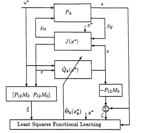
P i 2 M o
Least Squares
[image:32.529.61.476.91.674.2] [image:32.529.155.422.106.350.2]Figure 2-8: Model Reference Adaptive Control Special Case.
dependence is understood. Also, a unity gain feedback loop with open loop operator XV0i
is said to be well-posed when ( / -F W0i)~l exists. Recall that for a nonlinear operator S, then, in general S(A + B) ^ SA + S B, or equivalently superposition does not hold, and care must be taken in the composition of nonlinear operators. Otherwise, manipulation rules for nonlinear operators follow those more familiar ones for linear operators.
T h e o r e m 2.1
(Right fractional map forms) Consider that {AGo, K o } is well posed and stabilizing with left and right coprime factorizations for AGo, Ko as in (2.2.11,2.2.12) and the double Bezout (2.2.13) holding. Then any nonlinear plant with AG such that {AG, Ko} is a well-posed closed-loop system can be expressed in terms of a (nonlinear) operator S in right fractional map forms :
AG = N ( S ) M~ l {S); N{S) = (N0 + V0S), M(S) (2.3.1)
= AGo + M0"15 ( / + M0- 1a 0S )" 1M0- 1 (2.3.2)
Also, closed-loop system operators are given from
-1
1 & ___1 - l / - K 0 - l Uo Mo S 0
Vo Üo
= +
- A G I - A G o I Vo No 0 0 Nq M0
(2.3.3)
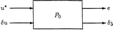
Moreover, the maps (2.3.1), (2.3.2) have the block diagram representations of Figures 2-9 (a) and (b) where
Jg
—Mq1Uq Mq1
Mo“ 1 AG0
2.3 Robust Nonlinear Control - Adaptive Q 23
The solutions of (2.3.1), (2.3.2) are unique , given from the right fractional maps in terms
of A G , or ( A G - A G 0) as
5 = { - N 0 + M 0A G ) { V o - Ü o A G ) - l
= M0(AG - A Gq) Mq[I - Üq( A G - AG0)M0]_1
or in terms of the closed-loop system operators as
— Nq Mq
I - K 0
- A G I
- l
I
-AGo
- K o
I
Moreover, [ N ( S ) , M ( S ) } are coprime and obey a Bezout identity
V0M ( S ) - UoN(S) = I
(2.3.5) (2.3.6)
1 _11
Mo
No
(2.3.7
(2.3.8)
P roof. Now simple manipulations allow (2.3.5) to be reorganized under the well-posedness assumption as
I
S
Vo -Üo
- N o Mo
I
A G
(I - K A G ) ~ 1Vq1
and via the Bezout identity, as
M ( S ) Mo + U0S
M0
Uo I IN ( S ) No +
y05
No Vo S A G( I - K A C ) - 1^ - 1
(2.3.9) Thus under (2.3.5) then M 1 (S') exists and,(2.3.1) holds as follows
N ( S ) M - 1(S) AG ( I - K A G ) - l V 0- 1 ( I - K A G ) - 1Vq1\ ‘ AG
To prove the equivalence of (2.3.1) and (2.3.2), simple manipulations give
AG = & G0 + ( N 0 + V0S ) ( I + Mö1UoS ) - 1Mq1 - N 0M ö l
= AGo + (Vo- N 0Mq1U0) S ( I + M o 1U0S ) - i M ü 1 = AGo + (Vo - Mq1NoUo) S ( I + Mq1UoS ) ~ 1Mq1
= AGo + Mq1S ( I + Mq1UqS ) ~1Mq1
so that under (2.2.13), then (2.3.2) holds. Likewise (2.3.5) is equivalent to (2.3.6) as follows
S = M 0( A G - A G 0){V0 - U0A G ) ~ l
= M0{AG - AGo)M0(V0Mo - UoAGM0)~l
= M0{AG - A Gq)Mq{I + ÜqNqMq1 Mq- Ü0AGMo)~l
= Mq(AG - A Gq)Mo[I - Üq(AG - AG0)M0]_1
To see that the operator of (2.3.1) is equivalent to that depicted in Figure 2-9(a), ob serve from Figure 2-9(a) that l = M j'^ e i - UqSI) , or equivalently, l = (Mo + UoS)~l e.
Also, (e2~W2) = (Nq + VqS)1 = {Nq + VqS )( Mq-I- UoS)~l e\ which is equivalent to (2.3.1).
Now suppose there is some other (5 + AS ) which also satisfies (2.3.1), then
I
I
---A G
l_________
7
JNq V0 I
S
(M0 + U
I
S + AS
(M0 + U0S + U 0A S ) ~ l
for some A S . Then, using (2.2.13),
Vo -Uo I I
- N o Mo AG S
(Mo + UoS)-1
l
S + AS
(Mo + UoS + Vo &S)-1 (2.3.10)
2.3 Robust Nonlinear Control - Adaptive Q 25
To verify (2.3.7), first observe that
1
----0
1
1___
M0 -Uo I 0
- A G / -N o Vo - S I
Thus
I -K o
- l
/ -K o
AG I - A G 0 I
M0 + U0S 0
0 Vq
I 0 - 5 /
Mo 0
Mo + UqS 0 - i
0
Vo
0
Vq
Mo -Uq
- Nq Vq
Mo Uo
No Vo
0 0
S 0
Mo -Uo
-N o Vo
(2.3.11)
- i
and applying the double Bezout (2.2.13)gives
Vo -Uo I -K o
- l
I -K o
-l-M0 -Uo 0 0
-N o Mo -A G I -A G o I -N o Vo 5 0
,or equivalently (2.3.3) holds, and (2.3.7). (This result is generalized in Theorem 2.2) Simple manipulations from Figure 2-9(b) give the transfer function of the G block to be 721*5(1 — J n S ) -1 J12 -I- 722, and substitution of (2.3.4) gives AG by (2.3.2).
To establish coprimeness of N( S) , M( S) observe that under the double bezout (2.2.13)
V0M( S ) - ÜoN(S) = V0M - Ü0N + (W o - Ü0V0)S = I
which is unimodular, Thus from [47] Lemma 2.1, N(S )M (5 )-1 is a right co-prime factor ization.
I
Remarks
2. The fact that Mo, No, Mo, No , Üo, Vo, Uo, Vo are linear has allowed derivations to take place without differential boundedness or other such assumptions as in a full non linear theory as developed in [46], [47] using left coprime factorizations.
3. Dual left coprime factorization results , apart from those in [46], [47] involving dif ferential boundedness, are elusive at this time. Certainly dualizing certain of the above proof steps requires superposition and thus linearity of AG. 5.
4. Dual results apply for fractional mappings of K = K (Q), as in (2.3.12),(2.3.13) along with duals of the other results. Thus K(Q) can be expressed as a linear controller
Ko augmented with a non-linear Q.Also, by duality, Figure 2-9(a) depicts a block diagram arrangement for
K £ K(Q) = U (Q )V-H Q y, U(Q) = (U0 + M0Q ),V(Q ) = (V0 + N0Q) (2.3.12)
where
Q = ( - U 0 + V0K )(M 0 - N „ K ) - 1 (2.3.13)
Stabilization R esults
We define a system {G, K } to be internally stable iff for all bounded inputs, the outputs are bounded.
T h e o r e m 2.2
Consider the well-posed feedback system {AG , K } under the conditions of Theorem 2.1, with AG and K parameterised by S,Q as in (2.3.1), (2.3.12) and as depicted in Figures 2-9 (a) and (b). Then (A G (5), K( Q) } is well posed and stable if and only if the feedback system {Q, 5} depicted in Figure 2-10 is well posed and internally stable. Moreover, referring to Figure 2-9(c), the Jfc/AG block with input/output operator T satisfies
T = S (2.3.14)
Proof. Observe th at from (2.3.1),(2.3.12)
I - K ( Q )
r
--— 1§
i___
Q > l I___
M o d- UqS 0
- A G(5) I
i
£
£
l
___
l - S I 0 Vq4- NqQ
2.3 Robust Nonlinear Control - Adaptive Q 27
Clearly, under the double Bezout identity (2.2.13), or equivalently under {AGo, A^o} well posed and internally stable,
I - K ( Q )
- l O
*
1
^—
i
exists <=>
- A G(S) I - S I
- l
exists.
Equivalently, {G(S),AT(Q)} is well posed if and only if {Q,S} is well posed. Thus under well posedness assumptions, taking inverses in, and exploiting (2.3.15) then simple manipulations yield
/ - K ( Q )
- A G(S) I
M0 0
i
----o
1
__
S 0 '
I - Q
- l
C0 Oo
+
0 C0 0 No 0 Q - S I No Mo
(2.3.16) r~ ---0 1 ^— i 1 __ __ __ - l
U0 M0 S 0 I - Q
-1
Co Uo
= 4
-- A G 0 I C0 No 0 Q - S I No M0
(2.3.17)
Now internal stability of {AGo, Ko} , {S, Q}, and stability of No, Nq etc leads to internal stability of the right hand side and thus of {AG(S), K{Q)} as claimed. Moreover from (2.3.17),(2.2.13)
S 0 I - Q
0 - S I
— N q Mq I - K ( Q )
«IA
1 - A G(S) I
I -K o -11 M0 -Uo
AGo I -N o Co
Thus well posedness and internal stability of {AG(S), K(Q)} and {AGojA'o} gives well posedness and internal stability of {Q,S} to complete the first part of the proof.
Now with Jk defined as in (2.2.17) then the operator T in Figure 2-9(c) can be represented as
T = V f l A G ( I - V ^ Ü o A G r 1^ - 1 - N0V0- 1 (2.3.18)
= V0- l &G(V0 - Ü o A G ) - l - N 0V0- '
= M o [ A G - A G o j(V b -^ o A G )-1 = 5
I
Rem arks
1. Note that this proof does not use superposition associated with operators S, Q,
but does in regard to Mo, No etc. The results following Theorem 2.1 also apply for Theorem 2.2. Thus the proof approach differs (of necessity) from the proof approach given in [64] for the linear S, Q case based on work with the left factorizations , since when working with left factorizations, superposition is used associated with the operators Q, S.More general versions of this approach where Go, Kqare nonlinear
will be explored in subsequent work.
2. If |5| < e then by the small gain theorem for closed feedback loops, if |Q| < 1/e then
Q stabilizes the loop. From this, and Theorem 2.2 with (AG — AGo) suitably small in norm, then there exists some Q which will guarantee stability.
3. In the case where AG = AGo then trivially 5 = 0 , and any Q selection based on identification of S will be trivially Q = 0. This contrasts the awkwardness of one alternative design approach which would seek to identify the closed-loop system as a basis for a controller augmentation design.
4. Observations on examples in the linear AG case have shown that if Ko is robust for G, then 5 can be approximated by a low order system [67], so making any Q
selection more straightforward than might be otherwise expected.
5. In [76] stability results are studied for nested linear systems based on the Q / S
parametrization approach. The authors demonstrate how an (n 4- 1) loop control diagram can be specialised to an equivalent n —loop diagram, and shows that internal stability of an (n -I- 1) control loop is equivalent to that of the controller in the last loop stabilizing the n-th frequency-shaped plant-model error. It is clear that our results could also likewise extend, at least in the case when all approximations but the last were linear.
2.4 Robust Nonlinear Control - Adaptive Q 29
regulator, then the adaptive regulator K (Q k) converges to Kq= K{0), the optimal one.
Such details are studied in [63]. More general results are given in [74] for the case of linear AG, based on an averaging analysis. One result concerns the case for when {AG, A^o} is a stabilizing pair, as well as {AGo,Ro}- There is guaranteed performance enhancement when {AG, Kq] is not stabilizing, but is small in that {AG, K{Q)} is stabilizing for some
Q with IIQII < e with e known, then with Qk projected into the domain {||Q|| < e),
there is guaranteed performance enhancement. For the more general case where AG is nonlinear, then new results are needed. One approach is the averaging analysis as used in [74] but for nonlinear systems as in [38], but clearly any results obtained will be problem specific and beyond the scope of this thesis. A first step in such an analysis is to derive appropriate stability results. Stability results for the proposed scheme in the nonlinear AG, but linear Ko, A Gqcase are studied in the next section. These are more developed
than those for the nonlinear Ko, A Gq, AG studied in references [46],[47]. Convergence
results for a learning-Q approach for linear systems as in Remark 8 in Section 2, would follow similar lines to the adaptive-Q approach, at least when AGo, Jk and Qare functions only of x*. But in the more general case when the operators are functions of x, or 6x, a stabilization theory coping with nonlinear A Gq,Jk is developed in Chapter 4.
2.4
S im u lation s
In this section, we demonstrate the efficacy of our approach through simulation studies. Consider an optimal control problem based on the van der Pol equation
X\ = (1 — x \ ) x \ — X2+ U, X2 = * 1 , y — x l (2.4.1)
with xi(0) = 0, £2(0) = 1 and the performance index defined by 1
I = - [x\ + x \ - f v?)dt (2.4.2)
2
Jo
A second-order algorithm [27], using 400 integration steps, was adopted for the numerical solution of the open-loop optimal control signal u*. An arbitrary initial nominal control
u = 0 ,t E [0,5], was chosen. The value of the performance index was reduced to the optimal one in 4 iterations in updating u(-) over the range [0,5].
A G{S)
T = S
[image:41.529.61.468.122.681.2]2.4 Robust Nonlinear Control - Adaptive Q 31
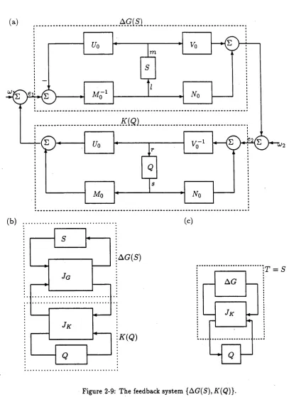
Figure 2-10: The feedback system {Q ,S }.
or a deterministic disturbance which disturbs the optimal input signal. Also, in some of the simulations we apply a plant with unmodelled dynamics. The objective is to regulate perturbations from the optimal by means of the index A I = Jq(Sx2 + 6x2 + 6u2)dt which is expressed in terms of perturbations <5x,<5u. For each of the disturbances added, and for the unmodelled dynamics case, we compare five controller strategies, and demonstrate the robustness and performance properties of the adaptive-Q methodology.
C ase 1: O p en -lo o p d esig n .
Here we adopt the optimal control signal u* as an input signal of the nonlinear system with added disturbance. Figure 2.11 shows that the open-loop design is quite sensitive to such disturbances in that xi , X2 differ significantly from x^x^.
C ase 2: L Q G ’s d esig n .
In order to construct feedback controllers, we adopt the standard LQG theory based on the linearized plant model of (2.4.1) about the optimal trajectories and the performance index (2.4.2). Of course, the input signals u* -1- 6u are no longer ‘optimal’ for the nominal plant. The LQG controller’s design yields better performance than the open-loop case in that the errors x\ — xJ, X2 — x\ are mildly smaller than in the previous figure for the open-loop case. See Table 2.4.1. It is well known, however, that the LQG controller, although optimal for the nominal plant model under the assumed noise environment, may lose performance and perhaps its stability even for small variations from the nominal plant model.
C ase 3: L Q G /L T R d esig n