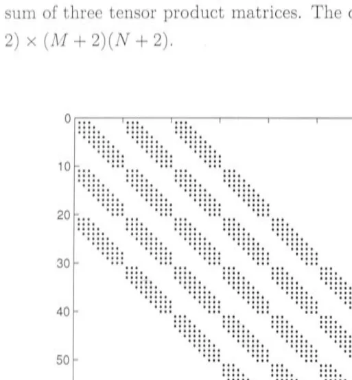
Finite element approximation of minimum generalised cross validation bivariate thin plate smoothing splines

(1)

Finite Element Approximation of

Minimum Generalised

Cross

Validation

Bivariate Thin Plate Smoothing Splines

PENELOPE HANCOCK BAPPSc(HoNs) The Centre for Resource and Environ111ental Studies

A thesis sub111itted for the degree of Doctor of Philosophy of t he Australian National University

(2)

D eclaration

T h e ·work in t h i:::; t h esis is 1ny O'Wll n11less other'ivi~e _{st.d.tecl .}

(3)

Acknowledgements

Throughout the course of this proj ect I have received help fron1 n1any generous people . Thanks first ly to Michael Hutchinson, for consistently and extensively supporting 111e throughout this project. Through our lengthy weekly meet-ings, I h ave been able to greatly advance 111y understanding of and interest in

co111put ational 111athe111atics. W ithout this help, the project would not have

been nearly so satisfying or so successful. Thanks also to · Frank deHoog, for 111onitoring the project and providing constructive advice throughout the last 3 years . The quality of this thesis has greatly improved as a result of this interaction.

I an1 also extremely grateful to Karl Jissen, whose assistance was vital in 111any a

16\'IEX

_{saga, and Barry Croke, who has been helpful for just about anything.}

Thanks to John Stein for help with GIS 111atters. And thanks to Ole Neilson, for answering rather vague questions about 111athe111atics in general, and to David Young, for generously providing

16\'IEX

wisdom .

JVIy experience at CRES has been 111ost enjoyable t hanks to the many friendly

(4)

Abstract

The application of thin plate srnoothing splines to the spatial interpolation of large data sets has in the past been limited by t he associated computa-tional cost . To obtain the analytic solut ion to the thin plate smoothing spline equations, O(n3) operations are required, making routine con1putation on the

average workstation infeasible for data sets with more than around 2000 data points. Methods for fast cornputation of analytic thin plate smoothing splines have been developed by past studies, and finite elen1ent approaches have also been widely en1ployed. These studies have investigated the t hin plate spline systen1 rnainly fron1 a numerical perspective , without an automatic mechanism for optirnising 'sn1oothness'. The srnoothness of a thin plate sn1oothing spline function is controlled by a sn1oothing paran1eter ,\. This parameter deterrnines how closely the data points are fitt ed. Depending on the value of,\, the data points can be exactly interpolated, or globally smoothed.

For practical sn1ooth spatial interpolation problems, surface sn1oothness is a central issue. The 1notivation for this study was the spatial interpolation of large environmental data sets, particularly climate data sets. Observations of environn1ental processes often contain a high noise component, so the extent to which the data are sn1oothed has a considerable influence on the predic-tive accuracy of the fitted function. Opti1nising the s1noothing para1neter by 1nini1nising the generalised cross validation ( GCV) is well known to be a suit-able n1ethod for 1ninin1ising the predictive error of the thin plate smoothing spline surface , and has been used in 1nany applications of thin plate smoothing splines . It was therefore the goal of this study to develop a co1nputationally efficient nu1nerical strategy for fitting approxi1nate 1nini1nu1n GCV thin plate sn1oothing splines to large data sets .

(5)

to deliver a user specified residual stun of squ ares fron1 the data. This

s111ooth-ness criterion is appropriate in the context of interpolating topography, where

an esti111ate of the data error is known. This study n1odifies the 111ethods ·in

Hutchinson [67], to iteratively obtain finite ele111ent approxi111ations to

111ini-111un1 GCV thin plate sn1oothing splines.

The procedure involved discretising the thin plate smoothing spline equ at ions,

and using a nested grid 111ultigrid iterative strategy to solve the discretised

system. The nested grid fra111ework facilitat es iteration on grids of varying

resolution, starting at a coarse resolution and sequentially refining the grids.

To opti111ise smoothness , the solution process incorporated a double iteration

to simult aneously update both the esti111ate of the discretised solut ion , and

the estimate of the mini111un1 GCV s111oothing para111eter. A Taylor series

expansion was used to esti111ate the value of ,,\ corresponding to the 111ini111u111

GCV. A stoch ast ic approxi111ation to the GCV was used to estin1ate the GCV

for given ,,\ values.

The investigations in this study led to an underst anding of the pro cess of double

iteration for t he case of the thin plate smoothing spline proble111 . It was found

that the it eration converged efficiently, except when the thin plate s111oothing

spline syste111 was poorly conditioned . Conditioning generally det erior ated as

the grid resolution was refined, particularly when the smoothing para meter was

large. Poor conditioning resulted in degr ad ation of the efficiency of the iter ative

processes. This caused the double iterat ion to becon1e poorly synchronised,

in that the solut ion estin1ate could not be efficiently adjusted in response to

changes in the s111oothing para111eter estin1ate. In these circu111stances the

double iteration did not always converge .

Throughout extensive testing of the procedure , a nu111ber of strategies_ for ov

r-co111ing the above proble111s were identified. Firstly, the type of discretisation

·was varied . Discretisation of the spline system using basis elen1ents co111pos d

of quadratic B-splines was foun d to stabilise the double iteration considerably

in con1parison to a sin1pler, piecewise constant discretisation. The

i111prove-1nent ·was attributed to the first order continuity of the quadratic B-spline

approxi1nation, which alluwed continuous, broadscale functions to be

accu-rately approxin1ated at coarse grid resolutions. Accurate methods of

transfer-ring quadratic B- plines fro1n coarse to fine grid resolutions also i111proved the

(6)

Convergence was further in1proved by appropriately setting the initial value of the ,.\ estin1ate, lin1iting the an1ount by which ,.\ could be updated, and en1placing suitable lower and upper bounds on the ,.\ estimate. A first order correction, applied to the solution estin1ate after each smoothing paran1eter update, was also found to i1nprove the perfonnance of the algorithm, by allow-ing the solution esti1nate to respond more quickly to the smoothallow-ing para1neter update. This depended on obtaining an efficient esti1nate of the derivative of the solution with respect to the s1noothing para1neter . The Taylor series expansion of the GCV in tenns of the s1noothing para1neter also used this derivative esti1nate .

(7)

I

Methods

1 Introduction

2

1.1

1.2

1.3

Overview and 111otivation .

Su111mary of the research process

Su111111ary of each chapter .

Smoothing splines

2.1

Univariate splines

2.1.1

Smoothing splines .

2.2

Thin plate s111oothing splines .

2.2 .1

Opti111isation using generalised cross validation (GCV)

2.2.2

Esti111ating the variance of the noise .

2.2.3

Interpretation of the signal .

2.2.4

Standard error estimates

2.2 .5

Geostatistical n1odels .

3 Discretisation of the univariate smoothing spline equations

3.1

Discretisation with piecewise constants

3.2

Discretisation with quadratic B-splines 3. 2 .1 _{B-spline fonnulation . . . .}

3.2.2

B-spline approximation of smoothing splines

4 Multigrid methods

4.1

Classical iterative methods

4.1.1

The weighted Jacobi method .

4.1.2

The SOR 111ethod . . . .

(8)

4.1. 3 Convergence . .

4. 2 The n1ultigrid 111ethod

4.2.1 Multigrid context

4.2 .2 History of multigrid developn1ent

4.2.3 The 111ultigrid principle

4.2. 4 Elen1ents of multigrid .

4.2.5 Guidelines for optin1ising the n1ultigrid

algorithm . . . .

4.2.6 Multigrid convergence

55

56 '56

58

61

67

68

5 Prolongation and -restriction of univariate quadratic B-splines 69

5.1 Hierarchial B-splines 69

5. 2 Prolongation . ₇₀

5.3 R estriction . . 72

5.3.1 The matrix X 73

5.3.2 The rnatrix Y 76

5.3 .3 The restricted solution 81

6 Discre tisation of the bivariate thin plate s1noothing spline

equa-tions ₈₃

6.1 Tensor product splines . . . . 84

6.2 Roughness penalty calculation 85

6.3 The total roughne s penalty . 103

7 Prolongat ion and rest riction of bivariat e quadratic B- splines 107

7.1 Prolongation . 107

7.2 R triction . . 112

8 Optimis ing the s moothing parameter 117

.1 Th OPTRSS algorith111 117

.2 Th 1\/IINGCV algorith111 121

.2.1 _{A tocha tic esti111ate for the trace of the influ nee n1atrix123}

.2.2 The algorithn1 . . . . 125

.2.3 Diff rentiation of Tr 125

.2. 4 An alternative for the bivariate ca e . 127

(9)

II

Results

₁₃₅

9 Testing of multigrid algorithms 137

9.1 Perfonnance of v-cycle and nested grid . 139

9.2 Application of the 1nultigrid principle _{. 146}

9.3 Different data sets . 154

9.4 Conclusion . . 157

10 Minimising GCV for the univariate piecewise constant smooth-ing spline system

10.1 Perfonnance of the OPTRSS algorith1n 10.1.1 The starting value of 0 .. . . .

10.1.2 The prescribed residual su1n of squares 10.1.3 The number of iterations per update .

10.1.4 The effect of fixing the smoothing para1neter to a lower value . . . .

10.2 P erfonnance of the MI GCV algorithm

10. 2.1 Stochastic error in the trace esti1nate 10.2.2 Da1npening the 0 updates

10.3 Conclusion . . . .. .

159

. 159

. 166

. 167

. 168

. 169

. 171

. 178

. 181

. 182

11 Minimising GCV for the univariate quadratic B-spline smooth-ing spline system

11.1 Stochastic error in the trace esti1nate 11. 2 A first order correction

11. 3 Different data sets

11.4 The convergence criteria

11.5 Iinproving the efficiency

11.5.1 Differentiation of Tr with respect to ,,\

11. 5. 2 Finite difference esti1nation of d

2

<Je~v

11.6 A 1nodified , i1nproved algorith1n 11. 7 Conclusion . . . . .

185

. 190

. 193

. 195

. 198

. 199

. 200

. 202

12 Minirnising GCV for the bivariate quadratic B-spline thin plate smoothing spline system

12.1 Results for different test data sets

205

(10)

12 .1.1 121.dat . . . .. . .. . .

12.1.2 Fr anke's principal test function 12.1.3 The peaks function

12.2 Conclusions . . . .

. 209

. 215

. 229

. 240

13 Performance of the MING CV algorithm for large t e mp erature

data sets _{24 3}

13 .1 Spatial interpolation of ten1perature data for t he African continent245 13.2 Spatial interpolation of temperature data for t he Australian

cont inent .. . . .

13 .3 The con1put atibnal saving 13.4 Conclusion .. . . .

14 Con clus ion

A Res ults for Chapt er 10

A. l _{Results generated by t he OPTRSS algorithn1 for the data set}

sine.dat

A.2 Results generated by the OPTRSS algorithn1, with a starting A

. 251

. 25 4

. 255

259

277

. 27

value of Ao

=

500 for the data set sine .dat . . . .. . . 2 0 A.3 Re ults generated by the OPTRSS algorithn1 ,vith a tarting A

value of Ao

=

5000000, for the dat a set sine.dat . . . 2 0 A.4 Re ult generated by t he OPTRSS algori thm, ,vith prescribed

S _{values of 2. 20 on each grid , for the data set sine.dat} _{. 2 0}

A.5 Re ults generated by the OPTRSS algorithrn ,vith a lo,, er thre

h-old on A update of A/ h3 _{for t he data et ine .dat . . . 2 2}

A.6 Re ults generated by the OPTRSS algorithn1: ,vith the 11100

h-ing para111eter fixed a A

=

5. for t he da a et ine.dat . . . . 2 4 /\_. 7 _{Re ult generated by t he l'vIIKGCV algorith111Jor the da a et}

ine.dat _{. 2 6}

A. Re ult generated by the :\II~GC algorithn1 for the da a et

ine .dat. u ing a econd rando111 vec or t . . . . 290

A .. 9 _{Re ult generated by the :\II:\"GC - algori h111 for he data} _e

ine.dat. for a third random vector t _{. 292}

A .. _{10 Re ult generated by the :\II:\"GC algori h111 u ing a damp}

(11)

B Results for Chapter 11

B. l Results generated by the MI GCV algorithn1, using quadratic B-spline discretisation

B.2 Results generated by the MINGCV algorithm, for a second ran-dom vector t

B.3 Results generated by the MI GCV algorithrn, for a third

ran-do111 vector t

B.4 Results generated by the MINGCV algorith111 , using the average

303

. 304

. 310

. 316

of 10 different rando111 vectors t . . . 319

B .5 Results generated by the MINGCV algorithm, applying a first

order correction to the solution esti111ate . . . . 325

B.6 Results of using the first order correction, for a second rando111

vector t . . . . 331

B. 7 Results of using the first order correction, for a third rando111

vector t . . . . . 337 B.8 Results generated by the MI GCV algorith111 , for the data set

bun1py.dat . . . 340

B.9 Results using the first order correction for the data set bu111py.dat346

B.10 Differentiating Tr with respect to

e

and

>- . . .

352

B.11 Results generated by the MINGCV algorith111 for the data set

sine.dat, with finite difference calculation of d2GCV/ d02 and

the convergence criteria emplaced . . . . 353

B.12 Results generated by the 111odified MINGCV algorith111 for the

data set bu111py.dat, with the convergence criteria e111placed. . 354

C Results for Chapter 12 357

C. l Results generated by the bivariate MINGCV algorith111, for the

data set 121.dat . . . 357

C.2 Results generated by the bivariate MINGCV algorithm , for the

data set frankel .dat . . . 359

C.3 Results generated by the bivariate MINGCV algorith111, for the

data set franke2.dat . .. . . 359

C.4 Results generated by the bivariate MINGCV algorithm , for the

(12)

C.5 Results generated by the bivariate MINGCV algorithn1 , for the

data set franke4 .dat . . . .. . . 362 C.6 Results generated by the bivariate MINGCV algorithm , for the

data set p eaks .dat . . . 364 C. 7 Results generated by the bivariat e MI GCV algorit h1n, for the

data set peaks15 .dat . . . .. 365 C.8 Results generated by the bivariate MIN GCV algorithm, for the

data set p eaksO.dat . . . 367

D Results for Chapter 13 371

D .1 R esults generated by the bivariate MI GCV algorithm , for the

African temperature data set . . . . . 372 D.2 Results generated by the bivariate MINGCV algorith1n for the

African temperature dat a set, with an init ial grid resolution of

25.6° . . . .. . . 374 D. 3 Results generated by the bivariate MINGCV algorith1n , for the

(13)

List of Figures

1.1 Stages in developing the algorithm to iteratively solve for

dis-cretised minin1um gen eralised cross-validation t hin plate

smooth-ing splines . . . .

1.2

1.3

The pro cess X . .

Noisy d ata observations of the process X.

1.4 Smoothing spline fit to data observations using a s1nall

smooth-12

14

ing p ararneter. . . 15

1.5 Smoothing spline fi t to data observations using a large

smooth-1.6

ing p ar am eter . . . .

The GCV as a function of the smoothing paran1eter , for the

15

data set in Figure 1.3. . . 16

1. 7 Sn1oot hing pline fit to data observations using the minimum

GCV sn1oothing p ararn eter. . . 16

1.

1.9

Piece,i\ ise constant discretisation on coarse and fine grids .

A quadratic B-spline b asis elen1ent . . . . . .

1.10 The pro ces of const ructing a quadratic spline by summing a

linear co111bination of t h e basis ele111ents .

1.11 The 111ultigrid process of tran £erring t h e solution esti111ate to

and fro111 grid of varying coarsen ess . . . .

1.12 A bivariate quadratic B-spline basis element .

1.13 The proces of double iteration obtaining increasingly accurate

estin1ate of the olution u and the 111inirnun1 GCV smoothing

paran1eter ,\ . . . .

1.14 The oscillatory behaviour of ,\ updates .

1.15 Divergent o cillatory behaviour of ,\ updates.

18

19

21

22

23

24

(14)

2.2

2.3

2.4

Srnoothing spline fit to noisy data . . . . . .

Thin plate sn1oothing spline fit to bivariate noisy data ..

Variograrn cornponents. .

31

34

40

3.1 The unidin1ensional grid. 42

3.2 B-splines of varying orders. 46

3.3 Polynon1ial pieces of a quadratic B-spline, with Wr ranging

fron1 0 to 1 on each knot interval. . . 48

3.4 _{Positions of quadratic B-spline basis elen1ents} _Br_{on the}

uni-3.5

4. 1

di111ensional grid. . . .

Quadr at ic B-Eipline b asis elements on coarse and fine grids .

The 111odes w i .

4.2 _{R epresent ation of a given 111ode on a fine grid and a coarse grid}

49

52

60

( a d apted fro•111 Briggs[20]). . . 60

4.3 Grid schedule for the v-cycle algorithn1 . 65

4.4 Grid schedule for the nested grid algorith111 . 66

5.1 _{R efine111ent of a quadrat ic B-spline basis elen1ent .}

5.2 _{Overlaps of coarse grid b asis elements with surrounding coarse}

grid basis elen1ents .

5.3 _{Overlap of coarse grid b asis elen1ents vvith surrounding fin e grid}

basis elen1ents .

5 .4 _{P olyno111ial pieces of a quadratic B-spline, divided up into fine}

grid knot intervals, vvit h u r an ging fron1 0 to 1 on each kno t

70

. 74

. 77

interval. . . 7

6.1

6.2

6.3

T·wo din1ensional grid for t h e biva riate s111oothing pline .

Biva riat quadratic B-spline basi ele111ent . . . . . .

Centre po i tions of basis elen1ent that overlap ·with B 1 J.

6.4 _{Polynon1ial piece for a quadratic B-spline and it first and}

ccond d ri \Tatives , ·with ll ranging fron1 0 to 1 ov r ach knot

5

6

inter\-al. _{. . . .} ₉₀

6.5 _{C -ntre point of ba is elen1 nt in position at or n ar the dges . 92}

6.6 _{Edge and near edge po ition for the lo\,-er} 1 ft corner . . . 93

(15)

7.1 _{The process of prolongating biquadratic B-splines , where the}

x symbol corresponds to the centre point of a biquadratic B-spline basis elen1ent .

7.2 _{Position of t he non-zero entries in the tensor product matrix}

. 108

for prolongation of a bivariate quadratic B-spline. . . . . 112

7.3 _{Positions of non-zero entries in the tensor product matrix X}₂₀

X_{1 .} . . . . 114

7. 4 _{Positions of non-zero entries in the tensor product matrix Y}₂₀

Y_{1 .} . . . 115

7.5 The pro cess of restricting a biquadratic B-spline. 116

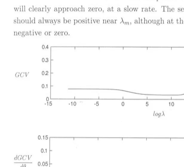
8.1 _{Plot of the GCV as a function of the logarith111 of the s111oothing}

parameter . . . . . 129

8.2 _{Plot of the GCV and its derivatives as a function of the}

loga-rith111 of the s111oothing parameter . . . . . .. . . 130

8.3 _{A closeup of Figure 8.2 , showing the region surrounding the}

111ini111u111 GCV . . .. .. . . .. . . 131

8.4 Plot of R _{and its derivatives as a function of the logarithm of}

t he s111oothing para111eter . . . 132

8.5 _{Plot of the signal and its derivatives as a function of the}

loga-9.1

9.2

rith111 of the s111oothing p arameter .

The d ata set sine.dat .

The analytic solution and the piecewise constant approxima-tion obtained using the v-cycle algorithm.

9.3 _{The analytic solution and the piecewise constant}

approxirna-133

140

. 141

tion obtained using the nested grid algorit hm. . . . . 141

9.4 _{The signal versus t he s111oothing para111eter for the data set}

sine .dat . . 142

9.5 _{The s111oothing spline solution corresponding to a smoothing}

para111eter of A= 50 . . . . . 142

9.6 Values of

tr( I - A)

and the GCV for different random vectors

t . . . .. .. . . 144

9. 7 _{The coefficient for each error mode VS the number of cycles}

(16)

9.8 The coefficient for each error 111ode VS the nu111b er of SOR

iterations for SOR iteration on the fin e grid, for the data set

sine .dat .

9. 9 lv1odes of e (0) corresponding to the 3 highest coefficients ci for

. t47

the data set sine .dat . . . . . 148

9.10 The piecewise constant solution on the coarsest grid and the

local averages of the data points in each grid cell, for the d ata

set sine.dat .

9.11 The piecewise constant solution on grid no. 6.

9.12 The piecewis~ constant solution on grid no. 5.

9.13 The piecewise constant solution on grid no. 4.

9.14 The piecewise constant solut ion on grid no. 3.

9.1 5 The piecewise constant solution on grid no. 2.

9.1 6 The piecewise constant solution on grid no. 1.

9.17 The data set 360. dat. . . .

9.1 8 The an alyt ic solution and the piecewise constant

approxima-tion obtained using the v-cycle algorith111 , for the data set

150

151

152

153

155

360 .dat. . . 156

9.1 9 The data set bumpy.dat . 156

9.20 The analytic solution and the piecewise constant

approxi111a-tion obtained using the v-cycle algorith111, for the data set

bu111py.dat . . . 157

10 .1 Successive s111oothing para111eter updates on grid no. 6

gener-ated by the OPTRSS algorith111, for the data set sine.dat. . 163

10 .2 Successive s111oothing parameter updates on grid no. 5

gener-ated by the OPTRSS algorithm , for the data set sine.dat . . 163

10.3 Succe sive s111oothing parameter updates on grid no. 4

gener-ated by he OPTRSS algorith111, for the data set sine.dat . . 164

10.4 Succes ive 111oothing para111eter updates on grid no. 3

gener-ated by the OPTRSS algorithm, for the data et sine.dat. . 164

10 .5 Succe ive 111oothing para111eter update on grid no . 2

gener-ated by the OPTRSS algorith111, for the data set ine.dat . . 165

10.6 Succe ive 111oothing para111eter update on grid no . 1

(17)

10. 7 Srnoothing spline solution for the data set sine .dat, with a fixed

smoothing parameter of 5.

10.8 OPTRSS solution on grid no. 2 for a fixed sn1oothing

paran1-. 170

eter of 5, for the data set sine.dat. . . . . 170

10.9 OPTRSS solut ion on grid no. 1 for a fixed sn1oothing

para1n-eter of 5, for the data set sine.dat. . 171

10.10 Successive s1noothing para1neter updates on grid 6 generated

by the MINGCV algorithm , for the data set sine .dat . . . . . . 175

by the MINGCV algorithm , for the data set sine.dat . . . . . . 175

by the MI GCV algorith1n , for the data set sine .dat. . . . . . 176

10.13 Successive sn1oothing para1neter updates on grid . 3 generated

by the MINGCV algorithm , for the data set sine.dat . . . . . . 176

by the MI GCV algorith1n, for the data set sine.dat . . . . . . 177

by the IVIINGCV algorith1n, for the data set sine.dat . . . . . . 177

11.1 Successive s1noothing para1nater updates on grid no. 6,

gener-ated by the MI GCV algorith1n, for the data set sine.dat. . 187

11.2 Successive smoothing paramater updates on grid no. 5,

gener-ated by the IVIINGCV algorithm, for the data set sine.dat. . 187

11.3 Successive sn1oothing paramater updates on grid no. 4,

gener-ated by the MI GCV algorith1n, for the data set sine.dat. . 188

11.4 Quadratic B-spline approxi1nation to the smoothing spline

so-lution on grid 6, generated by the MINGCV algorith1n for the data set sine .dat .

11.5 Successive sn1oothing para1neter updates on grid no . 3, using

a first order correction to the solution esti1nate following each

0 update, for a second rando1n vector .

11.6 Successive s1noothing para1neter updates on grid no. 3,

with-out using the first order correction, for the second random

vec-. 188

. 194

(18)

11. 7 Successive smoothing parameter updates for grid 3, for the

data set bumpy.dat, without using the first order correction. 197

11.8 _{Successive s111oot hing parameter updates for grid 3; for the}

data set bu111py.dat, using the first order correction. 197

12.1 _{Analytic thin plate smoothing spline fit to the data set 121.dat . 210}

12.2 _{Biquadr atic B-spline fit to the data set 121.dat . . . .. . . 212}

12.3 _{Overlay of the biquadratic B-spline solut ion and the analytic}

solution for the data set 121. dat. . . . . 212

12 .4 Difference between the biquadratic B-spline solution and the

analytic solution for the data set 121.dat . . . . . 213

12.5 _{Contours of Franke;s principal test function , on the unit square. 216}

12.6 _{Analytic thin plate spline fit to the data set frankel.dat .} _{. 217}

12 . 7 Biquadratic .B-spline fit to the data set frankel.d at . . 217

12 .8 _{Overlay of t he biquadratic B-spline solut ion and t he analytic}

solution for t he data set fr ankel.dat . . . . .. . . .. . . 21 8

12.9 _{Difference between the biquadr atic B-spline solution and the}

analytic solut ion for the data set fr ankel .dat. . . 218

12.10 Analytic thin plate spline fit to t he data set franke2.dat. . 221

12.11 Biquadratic B-spline fit to t he data set fr anke2.dat . . 221

12.12 Overlay of the biquadratic B-spline solution and the analytic

solution for the data set franke2.dat. . 222

12 .13 Difference between the biquadratic B-spline solution and the

analytic olution for the data et franke3.dat. . . 222

12.14 Analytic thin plate spline fit to the data set franke3.dat. . 223

12.15 Biquadratic B- pline fit to the data et franke3.dat . . 224

12 .16 Overlay of the biquadratic B-spline solution and the analytic

olution for the data et franke3.dat. _{. . . . 224}

12.17 Difference bet\Yeen the biquadratic B- pline olu ion and the

analytic olution for he da a et franke3 .dat. . . 225

12 .1 A..nalytic thin plate pline fit to the data et franke4.dat . . 226

12.19 Biquadra ic B- pline fit to the da a et franke4.da . . 227

12 . 20 O\·erlay of the biquadratjc B- pline olu ion and the anal ·tic

(19)

12.21 Difference between the biquadratic B-spline solution and the

analytic solution for the data set franke4.dat . . 228

12.22 The peaks function . . . 230

12.23 Data point positions for the data set peaks .dat. . 231

12 .24 Analytic smoothing spline fit to the data set peaks.dat. . 231

12.25 Biquadratic B-spline fit to the data set peaks .dat . . 232

solution for the data set peaks.dat. . .. . . 232

12.27 Difference between the biquadratic B-spline solut ion and the

analytic solution for the data set peaks.dat. . . 233

12.28 Analytic thin plate spline fit to the data set peaks15.dat. . 235

12.29 Biquadratic B-spline fit to the data set peaks15.dat. . . 235

solution for the data set peaks15.dat. . . . . 236

analyt ic solution for the data set peaks15.dat. . .. . . 236

12.32 Analytic thin plate smoothing spline fit to the data set peaks0.dat.

238

12.33 Biquadratic B-spline fit to the data set peaks0 .dat . . 238

solution for the data set peaks0.dat . . . . . 239

analytic solution for the data set peaks0 .dat . . . 239

13.1 Data point lo cations for the African ternperature data set . . 246

13.2 Minin1u111 GCV biquadratic B-spline surface representing

an-nual 111ean 111axi111um temperature , standardised to sea-level ,

for the African continent . . . 248

13.3 Surface produced by the bivariate MINGCV algorith111 for the

African te111perature data set, with initial grid resolution 25.6°

instead of 16°. . . 250

13 .4 The two grids used to cover the African continent and avoid

(20)

13.5 _{Co1nbination of temperature surfaces produced by the bivariate}

I'v1I1 GCV algorithm for the top and botto1n segn1ents of the

African continent . . . . . .. . . ·252 13.6 _{Data point locations for the Australian temperature data set.} ₂₅₃

13. 7 1v1inimum GCV biquadratic B-spline surface for mean annual

temperature, standardised to sea level, for the Australian con-tinent . . . . . .

13.8 Niap showing the surface in 13. 7.

. 257

(21)

List of Tables

9.1 Initial 111ultigrid settings . . . . . 138

9.2 A con1parison of output statistics for nested grid , v-cycle and

the analytic solution.

9.3

tr(I - A)

values after each iteration, for the nested grid

algo-rith111. • • • • • • • • • • • • • • • • • • • • • • • ,l . • • • • •

9.4 R values after each iteration, for the nested grid algorithn1.

. 140

. 145

9.5 CCV values after each iteration , for the nested grid algorith111. 145

9.6 Spectral radius of SOR iteration 111atrix for the data set sine.dat.

149

9. 7 Condition nu111ber of the 111atrix pT P

+

_{1~ QT Q}for the data set sine.dat.

9.8 Direct solut ion on coarsest grid , with different nu111b ers of grid

. 149

levels in the v-cycle algorithn1. . . 154

10.1 Prescribed residuals on each grid level, with CCV and signal

values .

10.2 Results generated by the OPTRSS algorith111 for the data set

sine .dat .

. 161

. 162

10.3 R esults generated by the OPTRSS algorith111, with a lower

threshold on A updates of A/ h3

₌

_{0.5 , for the data set sine.dat. 168}

10.4 Results of the OPTRSS algorithn1, with residuals prescribed to

correspond to a fixed sn1oothing para111eter of 5, for the data

set sine.dat .

10.5 Results generated by the MI CCV algorith111 , for the data set

sine.dat.

. 171

(22)

10.6 _{GCV values for the piecewise constant approximation to the}

s111oothing spline on each grid, for different prescribed

smooth-ing parameters , where local mini111a are e111phasised . . . . . '178

10. 7 _{Results generated by the MI GCV algorithm for the data set}

sine .dat, using a second rando111 vector t. . .. . . 179 10.8 _{GCV values for the piecewise constant approximation to the}

sn1oothing spine on each grid , for different prescribed sn1ooth-ing parameters , for a second rando111 vector t . Local 111ini111a

are emphasised . . . 179

10.9 _{Results generated by the MI GCV algorith111 for the data set}

sine .dat, for a third rando111 vector t.

10.10 GCV values for the piecewise constant approximation to the smoothing spline on each grid, for different prescribed smooth-ing parameters , for a third rando1n vector . Local minima are

. 180

emphasised. _{. .. .. . . .. .. . . .. . . 181}

10 .11 R esults generated by the MIN GCV algorithm for a dampening

factor of 1/2, for the data set sine.dat . . . . . .. 182

11.1 _{R esults generated by the Mll GCV algorith111, using quadratic}

B-spline discretisation. . . 186

11.2 _{GCV values for the quadratic B-spline approximation to the}

s111oothing spline on each grid , for different smoothing

para111-eters. Local 111inima are e111phasised . . . 1 9

11.3 _{Stochastic GCV e timate calculated using analytic thin plate}

splines , for 9 different rando111 vectors t and for different

smooth-ing parameters.

11.4 _{Results generated by the MINGCV algorith111, for a second}

rando111 vector t .

11.5 _{GCV values for the quadratic B- pline approxi111ation to the}

111oothing pline on each grid, for different pre cribed mooth-ing parameter , for a econd random vector t. Local mini111a

190

. 191

are e111pha i ed . . . . . 191

11.6 Re ult generated by the :VII\""GC - algorithm for a third

(23)

11 . 7 GCV values for the quadratic B-spline approxin1ation to the

sn1oothing spline on each grid, for different prescribed

srnooth-ing para111eters, for a third rando111 vector t. Local minima are

e111phasised . . . . . .. .. . . 192

11.8 Results generated by the MINGCV algorith111, using the

av-erage of 10 different rando111 vectors to calculate stochastic

esti111ates of the signal and the GCV. . . . . 192

11.9 Results generated by the JVIINGCV algorith111, applying a first

order correction to the solution after each

e

update. . . . . 193

11.10 Results generated by the MINGCV algorith111, for the data set

bu111py.dat . . . . . 196

11.11 Results generated by the MINGCV algorithn1, for the data set

bu111py.dat, applying the first order correction to the solution

after each

e

update . . . . . .. . . 196

11.12 D values for different grids, for the data sets sine .dat and

bu111py.dat . . . . . .. . . 198

12.1 Sun1111ary statistics for the analytic thin plate spline fit to

121.dat. . . . . 210

12.2 Results generated by the bivariate MINGCV algorithm for the

data set 121.dat. . . . . 211

12 .3 Sobolev nonn values after each iteration for 121.dat, before the

first

e

update is performed . . . . . 211

12.4 Sun1n1ary results for the analytic thin plate spline fit to frankel.dat.

216

12.5 Results generated by the bivariate MINGCV algorith111 for the

data set frankel.dat. . 219

12 .6 Sun1n1ary statistics for the analytic thin plate smoothing spline

fit to the data set franke2.dat . . . . . .. . . 220

12 . 7 Results generated by the bivariate MINGCV algorith111 for the

data set franke2.dat . . .. . .. . . 220

12.8 Su111111ary statistics for the analytic thin plate spline fit to the

data set franke3.dat . . . . . .. . . 223

(24)

12.10 Su111mary statistics for the analytic thin plate spline fit to the

data set fr anke4 .dat . . . . . .. 226

12.11 Results generated by the bivariate MINGCV algorithm for the

data set franke4 .dat . . . . . .. . . . .. . . 228

12.12 Su111111ary statistics for the analytic s111oothing spline fit to the

data set p eaks .dat. . . . . .. . . .. . . . 233

12.13 Results generated by t he bivariate MINGCV algorith111 for the

data set peaks .dat . _{. 233}

12.14 Su111111ary statistics for the analytic thin plate s111oothing spline

fit to the data set peaks15 .dat . . . . . 234

data set peaks15 .dat . . .. . .. . . .. 237 12.16 Results generated by the bivariate MI GCV algorith111 for t he

data set p eaks0 .dat . . .. . .. . . .. . . 240

12.17 Sum111ary statistics for the analytic thin plate spline fit to the

data set peaks0 .dat. . . . . .. . . .. . . . .. . . .. 240

13.1 Su111mary statistics generated by SPLI TB for the African

ten1-perature data set. . . 246 13.2 Results generated by the bivariate IVII TGCV algorithm for the

African te111perat ure data set . . . .. . . .. . . 24 7 13 .3 Results generated by the bivariate MINGCV algorith111 for the

African ten1perature data set, with an initial grid resolution of

25 .6° . _{. . . . .. . . .. . . .. . . 248} 13 .4 Results generated by the MIN GCV algorith111 for African

tem-perature data set, for the top section of the African continent . 249 13.5 Results generated by the MINGCV algorith111 for the African

te111perature data set, for the botto111 half of the African

con-tinent . _{. 250}

13.6 Su111111ary statistics generated by SPLI A for the Australian

t en1perature data et . . . . . .. . . 252 13. 7 Re ult generated by the bivariat -MI GCV algorithrn , for the

Au tralian ternperature data set.

B . l _{Re ult generated by the NII -GCV algorithrn, differentiating}

Tr \Vith respect to

e)

for grid 110. 6

. 254

(25)

B.2 Results generated by t h e MINGCV algorithrn, differentiating

(26)

Part I

(27)

(28)

Chapter 1 Introduction

1.1 Overview and motivation

The techniques involved in this study are designed to estimate spatially

de-pendent processes throughout a given region by spatially interpolating large nu111bers of noisy point observations of the process . The principal intended

application is the prediction of spatial processes that occur in natural ecolog-ical syste111s . Many natural processes, such as climate, topography, soil and

vegetation, have underlying spatial coherence, in that two observations that are close together are 111ore likely to have si111ilar values than two observations that are far apart. The interpolation procedure is designed to describe this

coherence, by finding spatially dependent trends in data observations taken at particular locations in the study area. Interpolation of these trends allows prediction at locations where 111easurements have not been taken. Interpolated values a1~e used to create regular two di111ensional grids of predictions , known

as surfaces , which can be incorporated into geographic information systems to visualise spatial patterns and detect spatial relationships. The appropriate resolution of the interpolated grid depends on the co111plexity of the process

and the density of the data.

(29)

1.1. OVERVIEW AND MOTIVATION

generally inadequately sampled and mapped, clirnate variables t hat are kno-\;vn to be correlated with plant and anin1al distributions are often used to predict vegetation characteristics. Bioclin1atic indices such as rainfall, temperature and solar radiation are widely known to discriminate between different veg-etation types, as de1nonstrated by Nix [93] and Mackey et al. [88]. Spatial interpolation of climate data has been shown to effectively predict spatial pat-terns in vegetation and agriculture

[71].

_{The use of interpolated surfaces to}

detect spatially varying trends also provides much needed spatially predictive, as well as descriptive capacity. In this way they are 1nore informative than other techniques of spatially mapping vegetation, such as aerial photography

-·

and remote sensing. Furthennore, ecosystem attributes do not always fonn distinctive and recognizable photographic patterns or spectral signatures [86]. Spatial interpolation of surface cli1nate variables is also an integral part of te1nporal cli1nate prediction via stochastic generation of climate data [64]. Elevation dependent spatially interpolated surfaces are used to predict long tenn spatial cli1nate variability . These techniques are linked to the develop-1nent of space-ti1ne stochastic weather 1nodels through the process of spatially extending the para1neters of point simulation 1nodels. Methodologies for con-structing such models are discussed in Hutchinson [63, 64] and Guenni and Hutchinson [43] .

The thin plate s1noothing spline 1nethod of spatial interpolation used in this study can be motivated by the following data model. Consider data obser-vations (zi, x1i, x2i, ... , xdi) 1neasuring a dependent variable _z and a set of d predictor variables x_{1 , . . . ,}xd . _{For exa1nple, surface climate is often well}

pre-dicted using latitude, longtitude and elevation. If it is assu1ned that z has both continuous long range variation as well as short range variation that is discontinuous and random, then we can propose the following 1nodel

i

=

1 .. . , n (1. 1)

where n _{are the nu1nber of data observations,}_g_{is a slowly varying continuous}

function and Ei are realisations of a random variable _E. _{The function}_g

repre-ents the patially continuous long range variation in the process measured by

zi . The error Ei are assun1ed to be independent with mean zero and variance

(30)

mi-CHAPTER 1. INTRODUCTION

croscale variation that occurs over a range smaller than the resolution of the

data set. The microscale variation may be spatially continuous, but the data

is not spatially dense enough to represent it, so it is usually assumed to be

discontinuous noise.

We airn to estimate the process g by a suitably continuous function f. The

function

f

must be able to separate the continuous signal g from the

discon-tinuous noise Ei. This function can be estimated by 111inirnising

(1.2)

over functions

f

E X, where X is a space of functions whose partial derivatives

of total order m are in £2 ( Ed) [113]. The

Ji

are values of the fitted function at

the ith data point, ,,\ is a fixed smoothing parameter, and

1:/'a

(J)

is a measure

of the roughness of the function

f

in tenns of mth order partial derivatives.

The form of

J!

(J)

depends on m and the number of independent variables d.

For example, if m = 2, which is a typical value, and d = 2, then

(1.3)

[113]. Expression (1.2) represents a trade off between fitting the data as

closely as possible whilst maintaining a degree of s111oothness. The smoothing

para111eter ,,\ controls the separation of signal and noise. If ,,\

=

0 the function

f

exactly interpolates the data, implying zero noise, where as if ,,\ is very large the function approaches a hyperplane. It is shown in Craven and Wahba [24]

that the. ,,\ corresponding- to the spline function

f

that best represents the

underlying process g can be accurately estimated by minimising the generalised

cross-validation, or GCV. The GCV is a measure of predictive error, and will

be discussed in Chapter 2.

The solution to this 111inimisation proble111 is well known to be a thin plate

smoothing spline function [99 , 31, 92, 113]. Multivariate thin plate splines

are not piecewise polyno111ial functions like the traditional univariate splines.

They are tenned 'splines' because the solution to (1.2) for the univariate case,

with m

=

2, is a natural cubic spline.

(31)

broad-1.1. OVERVIEW AND MOTIVATION

scale trends in noisy data is well documented in past studies over the last 20 years, in a wide variety of fields. The thin plate smoothing spline rnethodol-ogy is often an integral part of spatial modelling of environmental processes, including surface cli111ate processes [49, 63, 118], topography [58] remote sens-ing [10], pollutant dispersion [73] and plankton distributions [116] . They are also commonly used in other fields such as image analysis [11], medical re-search [83] and data mining [54, 53].

S111oothing splines have several attractive characteristics that explain their popularity across such a wide range of disciplines. They are robust in that accurate predictions ~an be achieved in the presence of significant data error. They are global in that they use information from all the data observations to calculate a prediction at any given location in the study area. Furthennore, the algorithms associated with smoothing spline co111putation are now effi-cient and operationally straightforward. Smoothing splines are also directly associated with a statistical framework that allows calculation of pointwise standard errors [113], _{as well as summary statistics such as the generalised}

cross-validation ( GCV) and the degrees of freedom of the fitted model. This facilitates quantitative assessment of the ability of the function to represent the underlying data generation process [ 63] .

To put thin plate smoothing splines in the context of other methods of spatial interpolation of noisy data vve can think of two approaches to smoothing noisy data. A p enalty term , such as

>.J!

(f)

_{can be added to the residual sum of}

squares tenn

t

L ~

₁

(zi - f i)

2 to impose smooth interpolation or the space of

functions that make up

f

_{can be restricted so that exact interpolation is not} po ible. For example -.ve could solve

ry 1

f

(x1 . x2)

=LL

Cjk in jx1 in kx2 j =l k=l

(1.4)

(1.5)

\\-here Cjk are the fi tted coefficient and x M

< <

n _{to achieve a low} dimen-ional bi-.-ariate Fourier ine erie fit hat smooth the data.

(32)

CHAPTER 1. INTRODUCTION

which constrain the form of

f (

x)

by considering only certain portions of the

data to generate predictions in a certain area. Techniques such as Thiessen

polygons [109] and deLauny triangulations [1] paritition the study area into small elen1ents and fit si1nple functions on each element. The data are exactly

interpolated on each element. These methods are not easily extended to higher

di1nensions [60]. There are also inverse distance weighting [101] and moving average methods [26, 91 , 82]. These 1nethods involve a subjective choice of weighting function , which is usually defined in terms of a radius of influence

beyond which data points are ignored [60].

The geostatistical method known as kriging is regarded as the main

competi-tor to thin plate splines as a method for spatial interpolation [25 , 60]. Kriging

originated in the mining industry, to help improve spatial esti1nation of ore

reserves [111]. Like splines, kriging is based on the model in ( 1. 1), but

as-sumes g is a realisation of a spatially correlated random furiction [7 4]. Both

splines and kriging have been shown by Kimeldorf and Wahba [79],

Math-eron [90] and Duchon [29 , 30] to be formally equivalent, although they are operationally different. Both generally provide higher predictive capacity than

the si1npler interpolation methods mentioned above, and require fewer

guid-ing covariates [63, 75]. They are also easily extended to higher dimensions,

although there are natural restrictions on the dimensions of the fitt ed surfaces

if they are to be robustly detennined fro1n observed data [22]. Splines tend

to be operationally simpler than kriging, because the kriging 1nethod requires

separate fitting and calibration of a spatial covariance structure [65].

As an example of thin plate smoothing spline interpolation of climate processes,

consider .the cases of temperature and precipitation. Thin plate smoothing

spline functions of latitude, longtitude and elevation have been shown to

accu-rately describe long term annual and 1nonthly mean surface temperature and

precipitation [57, 60 , 118, 119, 63 , 77]. Temperature is the simpler of the two

spatial processes, and has a roughly linear dependence on elevation that is

independent of location [60]. Hutchinson [60] de1nonstrated that the following partial spline model is a sensible model for temperature

(1.6)

(33)

measurement location i. _{The resulting solution incorporates a bivariate thin}

plate smoothing spline

f (

x, y) _{and a spatially constant linear trend on elevation}

with slope, or 'elevation lapse rate ' {3 .

Rainfall is a more complex and localised process than temperature, and it is not reasonable to assume a constant dependence on elevation throughout the study area. Rainfall can be accurately n1odelled by a thin plate spline with three independent variables, according to the following model

[57] . This allows for a spatially varying dependence on elevation. Other independent variables, such as slope and aspect, have been found to provide minirnal additional explanatory power [63] .

As rainfall is more spatially complex than temperature , it requires more data points for accurate prediction over a given area. Approximately 14000 points have been used to construct a reliable rainfall surface for the entire Australian continent , where as temperature surfaces have been constructed fro1n 1000 data points [60]. This raises the issue of computational efficiency, which has in the past been a major practical problem associated with thin plate s1noothing splines [119, _{54, 53]. The analytic calculation of thin plate s1noothing splines}

described in [113] requires O (n3

) operations, where n is the number of data

points . This method quickly becomes unworkable when the nu1nber of data points increases. To fit a thin plate s1noothing spline using 14000 data points would require a number of operations within an order of magnitude of 1012 . As a result, the production of a mean rainfall surface covering Australia by Hutchinson and Kesteven [70] required joining together a number of smaller urfaces. There are clearly many other spatial data sets that consist of thou-ands , or even millions , of data points. Also , one may wish to generate several urfaces for one process , corresponding to many different seasons or years. In this case , a fast , straightforward procedure is required.

This study ai1ns to ,viden the applicability of minimum GCV thin plate smooth-ing pline to the 1nodellsmooth-ing of climate and other environmental processes by increa ing the co1nputational efficiency of the spline fitting process. An opti-mal nu1nerical _{rategy ·who e co1nputational speed depended linearly on the}

(34)

computation. This corresponds to an O ( N) algorithm, where N is the number of unknowns. There are methods described in recent literature for fast

compu-tation of analytic thin plate smoothing splines for large data sets. Techniques

utilizing conjugate gradient preconditioning techniques [102] and ideas from 1nultipole expansions and Lagrangian junctions [8, 9, 7] calculate the analytic

thin plate smoothing spline solution to (1.2). These methods achieve

O(n)

workload, but involve co1nplex data structures and algorithms.

Finite element approaches have also been used in a nu1nber of studies,

in-cluding those by Terzopoulos [108], O'Sullivan [94] and Szeliski [106]. Ear-lier methods discuss discretisation of the roughness penalty, denoted above as

J!

(!),

fro1n the perspective of interpolation with minimum curvature [18, 105] . Hegland et al. [53] also present a methodology for calculating discrete thin plate s1noothing splines based on first order techniques similar to mixed finite

element techniques for the biharmonic equation [23, 50]. Similar techniques

were adopted by Ramsay [97], who presents an approach for bivariate spline

smoothing over complex domains.

All of these methods tend to focus on the numeric-analytic properties of thin

plate smoothing splines rather than their statistical properties, and therefore

do not incorporate an auto1natic 1nechanism for opti1nising smoothness. For

practical spatial interpolation problems, surface smoothness is a central issue

given that the data observations contain a significant noise component. The

amount of smoothing will affect the predictive accuracy of the fitted surface ,

so clearly it should be optimised. The smoothness of the fitted spline directly

corresponds to the ratio of the signal , or the effective nu1nber of parameters of

the fitted model, and the noise, or the degrees of freedo1n of the error [61].

Esti-1nates of the noise due to measure1nent error and microscale variation therefore

depend on the s1noothness of the fitted surface. Optimising smoothness also

provides insight into the variability of the data, and the scale and coherence

of the underlying data generation process.

The rninimu1n GCV criterion previously mentioned is generally appropriate for

opti1nising the smoothness of thin plate smoothing spline fits to noisy data [24 ,

113 , 62]. The GCV has been used to opti1nise smoothness for 1nost thin plate

smoothing spline applications to climate , eg. [57 , 63 , 118, 96 , 77]. Minimising

the GCV provides an objective criterion for co1nparing the predictive capacity

(35)

GCV surface can also be used to assess the reliability of the surface and its associated statistics [62]. For example , if the signal is equal to n, the spline has exactly interpolated the data and therefore has not separated the signal from the noise.

The primary objective of this study was therefore to construct a simple, fast , grid-based algorithm for calculating nun1erical approximations of t hin plate smoothing splines, incorporating procedures to minimise GCV. The intention was to make the process of optimising srnoothness as efficient as possible. A double iteration was therefore used to simultaneously produce increasingly ac-curate estimates of the minimum GCV smoothing parameter and the s1nooth-ing spline solution. Such a process would be considerably faster than fully solving the spline equations for a numb er of different levels of smoothness in order to find t he optimal solution.

Hutchinson [58, 67]_ developed a simple multigrid based strategy which calcu-lates finite element approxi1nat ions to thin plate smoothing splines for elevation data in O(N) operations, where N is the numb er of grid points . This method emphasises the statistical framework of thin plate sn1oothing splines [61], and optimises smoothness to yield a user specified residual su1n of squares. This criterion is appropriate in t he context of interpolating topography, where an estimate of the amount of noise is available [58]. A study by Altas et al. [2] showed that multigrid methods are very efficient for solving a finite difference discretisation of the biharmonic equation , whilst standard iterative methods such as J acobi and Gauss-Seidel exhibit very slow convergence. The discretised thin plate smoothing spline equations have a similar structure to the discre-tised biharmonic equation, as discussed in Chapter 6. The results of Altas et al. [2] therefore indicate that the success of the Hutchinson [58, 6?] method is largely due to the use of 1nultigrid techniques .

(36)

of this study is given below. Hancock and Hutchinson [48], a publication re-sulting from t his study, presents results of in1plen1enting the methodology to approximate minimum GCV univariate smoothing splines.

1.2 _{Summary of the research process}

The process undertaken to obtain the discretised minimu1n GCV thin plate s1noothing splines is shown in Figure 1.1. The thin plate s1noothing spline

equations were first discretised to allow the solution to be approximated by a series of discrete ele1nents. Various multigrid iterative schemes were then tested with the aim of selecting an optimal method for solving for the coefficients of the discretised system. Additional procedures were then incorporated to allow simult aneous solution of the system and optimisation 9f s1noothness by 1nini1nising G CV.

Although this study is interested in bivariate thin plate smoothing splines, 1nuch of t he early algorith1n analysis and development was done for the univari-ate case . This was because the process of testing and optimising the methodol-ogy was 1nuch si1npler and more transparent in one dimension. The results of the univariate testing provided guidelines for the development of the bivariate algorit h1n.

The methods involved in the three stages in Figure 1.1 were continually re-fined t hroughout the preliminary univariate analysis. A numb er of different approaches were investigated and optimal strategies were selected. The most i1nportant progression was the type of discretisation. The system was origi-nally discretised using piecewise constants. Further analysis indicated that a quadratic B-spline discretisation was better suited to the t hin plate smoothing spline equations, due to its ability to represent smooth processes at coarse grid resolutions . This progression explains the chapter organisation for this thesis .

1.3 Summary of each chapter

(37)

1.3. SUMMARY OF EACH CHAPTER

full procedures are explained in detail.

PART 1: METHODS

The first part of the thesis presents the technical details of the methods used

1. Discretisation

Using piecewise constants and

quadratic B-splines.

2. Iterative solution

Using multigrid methods.

3. Optimisation

Using a double iteration to

simultaneously solve the discretised system and converge to a

minimum GCV solution .

[image:37.1193.192.670.355.963.2]

(38)

in this study, from the underlying thin plate smoothing spline model to

meth-ods of discretising the spline system, to the iterative algorithm for solving the

equations and optimising smoothness.

Chapter 2 - Smoothing splines.

The necessity of optimising the smoothness of spline functions fitted to noisy

data is easily depicted in the univariate case. Assume we want to estimate a

process X that has both smooth, broadscale variation and short range

varia-tion, as shown in Figure 1.2. We collect data measuring the phenomenon X,

shown in Figure 1.3. The data set contains significant noise due to

measure-ment error. Smoothing spline functions are ideal for representing the process

X from such data, as they can be used to detect broadscale trends that can

be reliably interpolated into data sparse regions.

The smoothing parameter ,,\ in equation (1.2) provides a lot of flexibility in

the way smoothing splines fit noisy data. A very small value of,,\ produces a

spline function that exactly interpolates the data, as shown in Figure 1.4. This

is clearly a poor representation of the process X because it incorporates the

errors in the data. Conversely, if the ,,\ value is too large, we can oversmooth

the data, as shown in Figure 1. 5.

One method of optimising the smoothness of the fitted spline to estimate the

process Xis to minimise the CCV. The CCV measures the predictive capacity

of the fitted spline by essentially determining how well the function predicts

withheld data. The CCV calculation implicitly involves removing each data

point in turn and sumrning, with appropriate weighting, the square of the

dis-crepancy of each omitted data point from a surface fitted to all other data

points. A plot of the CCV as a function of the logarithm of the smoothing

parameter for the data set in figure 1.3 is shown in Figure 1.6. Figure 1. 7

shows the result of 1ninimising the CCV to optimise smoothness for this data

set. The nu1nerical methods in this study ai1n to approximate this optimal

(39)

1.3. SUMMARY OF EACH CHAPTER 1.5 0.5 0 -0 .5 -1 -1 .5 -2

- 2.5 ~ - - - ' - - - - ~ - - - ~ - - - ' - - - ' - - - ' - - - - ~ - - - '

0 50 100 150 200 250 300

Figure 1.2: The process X.

2

+

1.5

>-++

1

>-+ + + +

++

0.5 ₊

+ + 0 + -0 .5 -1 -1 .5 -2 + + + + ++ +++ + + + + + + + + + + + + + + _{+ +} ++ + + + +

+ + -t: ++

++ + ++ + + + + + + +

+++ +-t+

+ + +++ + + + + + + + + + + + + 350 -/+ + + + +

-2 .5 ~ - - ~ - - - - ' - ' - - - - ' - - - ' - - - ' ' - - - ' - - - ' ---'

0 50 100 150 200 250 300 350

[image:39.1193.157.599.110.955.2]

(40)

CHAPTER 1. INTRODUCTION

2 ~ - - - , - - - - , - - - , - - - , - - - , - - - , - - - , - - ,

1.5 0.5 0 -0.5 -1 -1 .5 -2

-2 .5 c _ _ _ _ _ , _ _ _ _ ...,__ _ _ - ' - - - ' - - - - ~ - - - ' - - - - ~

0 50 100 150 200 250 300 350

Figure 1.4: Srnoothing spline fit to data observations using a small s1noothing parameter.

2 r - - - r - - - , - - - - , - - - , - - - , - - - , - - - , - - ,

1.5 0.5 0 -0 .5 -1 -1 .5 -2 + + ++ + + + + + ++ + +=+----+ ++ + + + + + + + + + + + + + + + + ++ + + + + + + + + + ++ ++ + ++ ++ + + + + +++ + + + + + ₊ + + +++ + + + + +

- 2 . 5 ~ - - ~ - - ~ - - - ' - - - ~ - - - - ' - - - - ~ - - ~

0 50 100 150 200 250 300 350

(41)

1.3. SUMMARY OF EACH CHAPTER

> u

(9

OB

0.7

0£

05

0.4

03

0 2 ' - - - ' - - - ' - - -

---'----__L_----5 0 5 10 15 20

log A

Figure 1.6: The GCV _{as a funct ion of the smoothing parameter ,} for the data set in Figure 1.3.

2

+

1.5 ₊ +

++

+ ₊

++ _{++ +}+ + + ++ ₊₊

+ + +

0.5

+ + + +

+ ₊

+ /+

0 + +

+ + ₊

+

-0 .5 + +

+ + +

-1 ₊ +

+. + +

-1 .5

+ + +

-2

+ +

-2.5

0 50 100 150 200 250 300 350

Figure 1. _{7: Smoothing spline fit to data observations using the}

Finite element approximation of minimum generalised cross validation bivariate thin plate smoothing splines