promoting access to White Rose research papers
White Rose Research Online
eprints@whiterose.ac.uk
Universities of Leeds, Sheffield and York
http://eprints.whiterose.ac.uk/
This is the author’s post-print version of an article published in the
Journal of
Computational Physics
White Rose Research Online URL for this paper:
http://eprints.whiterose.ac.uk/id/eprint/76342
Published article:
Cooper, JD, Valavanis, A, Ikonic, Z, Harrison, P and Cunningham, JE (2013)
Stable perfectly-matched-layer boundary conditions for finite-difference
time-domain simulation of acoustic waves in piezoelectric crystals.
Journal of
Computational Physics, 253. 239 - 246. ISSN 0021-9991
Stable perfectly-matched-layer boundary conditions for
finite-difference time-domain simulation of acoustic waves in
piezoelectric crystals
J.D. Cooper, A. Valavanis, Z. Ikoni´c, P. Harrison, J.E. Cunningham
Institute of Microwaves and Photonics, School of Electronic and Electrical Engineering, University of Leeds, Leeds, LS2 9JT, United Kingdom
Abstract
Perfectly matched layer (PML) boundary conditions are derived for finite-difference
time-domain analysis of acoustic waves within piezoelectric crystals. The robustness and
ef-fectiveness of the derived boundary conditions are demonstrated by simulating acoustic
wave propagation in the bismuth germanate material system—a system in which simple
absorbing boundary conditions cause instabilities. An investigation into the stability and
effectiveness of the PML is then presented in terms of the PML thickness and absorption
profile. A range of optimised absorption profiles were determined by finding the
maxi-mum permissible absorption within the stability limit of the system. In the optimised
case, the form of the absorption profile had little influence on the effectiveness of the
PML. However, in the unoptimised case the linearly increasing absorption profile was
found to be the most effective.
Keywords: Finite-difference time-domain, Acoustic wave, Perfectly matched layer,
Piezoelectric crystal
1. Introduction
The finite-difference time-domain (FDTD) method, introduced by Yee [1] in 1966
for simulating Maxwell’s equations, was first applied to the acoustic wave equations of
motion in piezoelectric crystals by Smithet al. in 2002 [2]. Since the solutions of both
these systems involve propagating waves, the method of truncating an otherwise infinite
Email address: el06jdc@leeds.ac.uk(J.D. Cooper)
simulation domain around some region of interest (ROI) is critical in stopping reflections
off these artificial boundaries interfering with the physics being investigated. In 2006,
Chaglaet al. [3] added absorbing boundary conditions to the acoustic wave problem by
adding an absorbing layer with a quadratically increasing damping coefficient to dissipate
the energy from any oscillations which reach the boundaries. Although this method
worked well in some cases, Chaglaet al. showed that it does not remain stable for all
material systems.
Since it was first introduced by Berenger in 1994 [4], the perfectly matched layer
(PML) has been used extensively in FDTD simulations of electromagnetic waves. It may
be viewed as an analytic continuation of spatial variables onto the complex plane such
that any oscillating solution that enters the PML will be transformed into an oscillating
component with an exponentially decaying envelope [5]. Despite the ongoing interest
in development of the PML [6, 7, 8, 9] in electromagnetic simulations as well as its
application in both elastodynamics [10] and fluid dynamics [11], the PML has not been
applied to the simulation of acoustic waves in piezoelectric crystals.
In this work, we derive PML boundary conditions for the acoustic wave equations
of motion within a piezoelectric crystal by applying a complex coordinate stretching of
spatial variables in the frequency domain. The boundary conditions are then transformed
back to the time domain and discretised using the same interlaced mesh used by Smith
et al. such that both the ROI and PMLs may be solved using the same FDTD algorithm,
thereby avoiding any increase in computational complexity in the simulation.
The robustness and effectiveness of our PML implementation is demonstrated in the
following section, and is shown to be stable for a bismuth germanate material system
in which absorbing boundary conditions fail [3]. This is followed by a discussion of the
stability criteria for the discretised PML and a quantitative analysis of their effectiveness
with respect to their operating parameters as well as optimisation of those parameters.
2. Derivation of PML boundaries for the acoustic wave equations of motion
The equation of motion for an acoustic wave in a piezoelectric crystal is
ρu¨i=
∂σij
∂xj
fori, j= 1,2,3, (1)
whereu is the displacement of a particle in three orthogonal directionsx1, x2 and x3,
and
σi=Cijj+eTik
∂φ ∂xk
fori, j= 1,2, . . . ,6;k= 1,2,3, (2)
is Hooke’s law for piezoelectric crystals, whereσ is the stress,C is the elastic constant
tensor, eT is the transpose of the piezoelectric constant tensor, φ is the induced
piezo-electric potential inside the crystal structure andis the strain inside the crystal which
is defined as
i =
∂ui
∂xi
fori= 1,2,3, (3)
4 =
∂u2
∂x3
+∂u3
∂x2
, (4)
5 =
∂u1
∂x3
+∂u3
∂x1
, (5)
6 =
∂u1
∂x2
+∂u2
∂x1
. (6)
Note that the subscript ofσhas changed from tensor notation in (1) to matrix notation
in (2), as in Ref. [12], so that both the wave equation and Hooke’s law may be expressed
using the Einstein summation convention.
The computational effort required for the simulation is greatly reduced by assuming
that the acoustic waves are of Rayleigh wave type, and therefore have no variation in
the direction aligned parallel to the propagating wave front. Taking this direction to
be along the x2-axis, all terms containing ∂x∂
2 may be set to zero. This reduces the
number of independent terms on the RHS of (1) to two, or in the summation notation
j= 1,3, and in (2) the number of independent equations reduces from six to five asσ2
is not used, so in the summation convention i = 1,3,4,5,6. The summations for the
equations of motion and Hooke’s law remain the same throughout the rest of this work
so will no longer be shown. While the variation in the x2 direction is assumed to be
zero the displacement in this direction direction,u2, is not zero and therefore cannot be
discounted. The problem may be simplified further if the solution is restricted to one
particular crystal class such that many of the terms in (2) become zero due to symmetries
within the crystal’s unit cell. In the following derivation however, all terms within (2)
have been included to make PMLs applicable to all crystal classes and therefore to be
material independent.
Since the acoustic velocity inside a crystal is slow compared to the piezoelectric
re-sponse, the induced charge displacement from the acoustic wave, ρ, is assumed to be
adiabatic and takes the form
ρ=−∇i·eijj fori= 1,3;j= 1,3,4,5,6, (7)
therefore allowingφto be found by solving Poisson’s equation
∇ ·ε∇φ=−ρ. (8)
In order to implement PML boundary conditions we split the second order time
differential by introducing an auxiliary field,v, such that (1) becomes
ρ∂ui ∂t =
∂vij
∂xj
, (9)
where the time differential ofv is defined as
∂vi
∂t =σi=Cijj+e
T
ik
∂φ ∂xk
. (10)
Transforming to the frequency domain, such thatu(t) → U(ω) and v(t)→ V(ω), we
obtain
−iωρUi=
∂Vij
∂xj
, (11)
and
−iωVi=Cijj+eTik
∂φ ∂xk
, (12)
respectively, whereω is the angular frequency of the acoustic wave. We now introduce
the complex change of variables such thatxi→(1 + iζωi)xi, whereζhas two components,
ζ1(x1) andζ3(x3), which are the absorption profiles of the PML in thex1andx3direction
respectively, to give
−iωρUi=
1
1 + iζj
ω
∂Vij
∂xj
, (13)
and
−iωVi=Ci1
1
1 + iζ1 ω
∂U1
∂x1
+Ci3
1
1 + iζ3 ω
∂U3
∂x3
+Ci4
1
1 + iζ3 ω
∂U2
∂x3
+Ci5
1
1 + iζ3ω
∂U1
∂x3
+ 1
1 + iζ1ω
∂U3
∂x1
!
+Ci6
1
1 + iζ1ω
∂U2
∂x1
+eTi1 1
1 + iζ1ω
∂φ ∂x1
+eTi3 1
1 + iζ3ω
∂φ ∂x3
.
(14)
Multiplying by (1 + iζ1ω)(1 + iζ3ω) gives
−iωρUi+ρ(ζ1+ζ3)Ui+
i
ωρζ1ζ3Ui= ∂Vij ∂xj + i ω ζ1
∂Vi3
∂x3
+ζ3
∂Vi1
∂x1
, (15)
and
−iωVi+(ζ1+ζ3)Vi+
i
ωζ1ζ3Vi=Cijj+e
T ik ∂φ ∂xk + i ω ζ1
Ci3
∂U3
∂x3
+Ci4
∂U2
∂x3
+Ci5
∂U1
∂x3
+eTi3 ∂φ ∂x3
+ζ3
Ci1
∂U1
∂x1
+Ci5
∂U3
∂x1
+Ci6
∂U2
∂x1
+eTi1
∂φ ∂x1
.
(16)
Transforming back to the time domain gives
ρ∂ui ∂t =
∂vij
∂xj
−ρ(ζ1+ζ3)ui+αi, (17)
where the auxiliary fieldαhas been introduced in place of the i
ω terms in (15), which
be-come time integrals when transformed to the time domain, such that the time derivative
ofαis
∂αi
∂t =ζ1 ∂vi3
∂x3
+ζ3
∂vi1
∂x1
−ρζ1ζ3ui, (18)
and
∂vi
∂t =Cijj+e
T
ik
∂φ ∂xk
−(ζ1+ζ3)vi+βi, (19)
where the auxiliary fieldβ has been introduced in place of the ωi terms in (16), such that its time derivative is
∂βi
∂t =ζ1
Ci3
∂u3
∂x3
+Ci4
∂u2
∂x3
+Ci5
∂u1
∂x3
+eTi3∂φ ∂x3
+ζ3
Ci1
∂u1
∂x1
+Ci5
∂u3
∂x1
+Ci6
∂u2
∂x1
+eTi1
∂φ ∂x1
−ζ1ζ3vi.
(20)
As identified by Smith et al. [2], the most natural choice of discretisation grid for
applying FDTD analysis to the acoustic wave equations of motion is an interlaced mesh,
with grid points interlaced in both space and time, as depicted in Fig. 1. Here,uandφare
mapped to whole-integer values ofx1,x3andt, whilev is mapped to half-integer values.
Applying the finite difference approximation, it then follows that a spatial derivative
depends upon the field values at±1
2, which lie in between grid points. Thesemidpoints
may be taken as the average of their adjacent points, i.e. for a spatial derivative in the
directionx1 at the point (i, k)
∂v ∂x1
(i, k) = ¯v(i+
1
2, k)−v¯(i− 1 2, k)
δx (21)
where ¯v represents the average of the neighbouring points, i.e.
¯
v(i+1 2, k) =
v(i+1 2, k+
1
2) +v(i+ 1 2, k−
1 2)
[image:7.595.124.489.176.503.2]2 (22)
Figure 1: The interlaced mesh FDTD lattice shown for three half-integer time points.
As is normal with FDTD analysis, the instantaneous values of time-dependent
vari-ables are sampled midway between the time steps used in evaluating time-derivatives,
such that (17) and (19) become
ρui|t+1−ui|t
δt =
∂v
ij
∂xj
−ρ(ζ1+ζ3)ui+αi
t+1 2
, (23)
and
vi|t+1
2 −vi|t−12
δt =
Cijj+eTik
∂φ ∂xk
−(ζ1+ζ3)vi+βi
t
. (24)
However, this implies a dependence on uand v at time steps between those to which
these variables are mapped (i.e. ui|t+1
2 in (23) andvi|tin (24)). This may be overcome
by first noting that these terms are zero within the region of interest and therefore any
approximation that is made will not affect what we are trying to observe except possibly
increase artificial reflections from the boundaries, and second realising that the difference
between the spatial derivative at half time steps should be small provided that a small
time step,δtis used. We therefore make the assumption that, in (23),ui|t+1
2 ≈ui|t, and
in (24),vi|t≈vi|t−1
2 and note that doing so does not produce a noticeable increase in
numerical noise from the PMLs in practice.
A similar problem arises when discretising the auxiliary fieldsαand β in time
αi|t+1
2 −αi|t−12
δt =
ζ1
∂vi3
∂x3
+ζ3
∂vi3
∂x1
−ρζ1ζ3ui
t
, (25)
βi|t−βi|t−1
δt =
ζ1
Ci3
∂u3
∂x3
+Ci4
∂u2
∂x3
+Ci5
∂u1
∂x3
+eTi3∂φ ∂x3
+ζ3
Ci1
∂u1
∂x1
+Ci5
∂u3
∂x1
+Ci6
∂u2
∂x1
+eTi1∂φ ∂x1
−ζ1ζ3vi
t−1 2
.
(26)
However, here the values ofuand vat the half time step may be taken as the average
of the adjacent time steps since they are already known, i.e.
ui|t−1 2 =
ui|t+ui|t−1
2 , (27)
and
vij|t=
vij|t+1
2 +vij|t− 1 2
2 , (28)
although we note, however, for simplicity, the same approximation as in (23) and (24)
may be used and in practice the PMLs still have the desired effect.
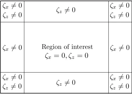
The simulation domain for time-dependent variables is terminated by hard-wall
bound-aries so that the simulation takes the form shown in Fig. 2. Forφ, Neumann boundary
conditions are implemented. The hard-wall boundary condition is implemented on the
whole-integer grid points, mapped to the variableu, meaning that the outside edge of
the PML, and therefore the maximum value ofζ, occurs at the half-integer grid points,
mapped tov, immediately inside of the hard-wall boundary.
The above derivation may easily be applied to the 3-dimensional acoustic wave
equa-tions of motion. However, in that case two (ωi)2 terms appear within the equations in
the frequency domain, which become second-order time integrals in the time domain.
Figure 2: Illustration of the simulation domain showing the PMLs at the edges of the region of interest and whereζis non-zero. Note that becauseζis zero within the region of interest the auxiliary fieldsα
andβare also zero here.
3. Numerical results
We present an example of a bulk wave propagating radially outwards towards PML
boundaries in the bismuth germanate (Bi4Ge3O12) material system. Chagla et al. [3]
previously showed that the use of boundary layers with quadratically-increasing
damp-ing coefficients led to instability in the simulated propagation of acoustic waves in this
material. By way of comparison, we show that our proposed PML equations provide a
stable and efficient means of absorbing incident waves.
Thex1- andx3-axes of the simulation are aligned along the [1,1,0] and [0,0,1] crystal
axes respectively by rotating the elastic and piezoelectric tensors by 45◦about the [0,0,1]
crystal-axis such that an acoustic wave will propagate along the [1,1,0] direction, as is
done experimentally with cubic crystals. The excitation frequency used was 1 GHz, as
in [3], making the spatial discretisation step,δx1 andδx3, 0.15µm (i.e.,∼ 20λ). The grid
size of the region of interest was set to 201×201 points and the time step,δtwas set to
25 ps observing the FDTD stability criterion [13]. The PMLs used were 10-points thick
(∼ λ
2) and the parameterζ was increased quadratically up to its maximum stable value
of 1.58×10¹⁰rad s−1 as described in the following section.
The acoustic wave was excited by setting a 3×3 square in the centre of the simulation
domain to have a constant charge which was then oscillated sinusoidally at the excitation
frequency for two periods and solving Poisson’s equation to find the potential profile
around this charge over the simulation domain. This potential profile was used as an
input to the acoustic wave equations of motion to launch a propagating wave. This
method of excitation was used firstly because it is more physically realistic than exciting a
component of the displacement since acoustic waves in piezoelectric crystals are generated
using an alternating potential, and secondly because excitations at a single point tend to
lead to instabilities caused by the change in sign of the spatial differential from the point
of excitation to its surrounding points. These instabilities manifest themselves as changes
in the sign of the solution from one grid point to the next such that the entire solution
appears modulated by a sawtooth wave with oscillations of the order of the grid spacing.
Fig. 3 shows the resulting acoustic wave propagating in bulk bismuth germanate, with
material parameters taken from [14], which is absorbed by the PML boundaries.
4. Stability and optimisation of the PML
The discretized PML equations will be subject to a system-dependent stability
cri-terion, much the same as the stability criterion for the unmodified equations within the
region of interest. Considering the stability criterion for FDTD analysis in two
dimen-sions [13]
vmaxδt=
1
δx2 1
+ 1
δx2 3
−12
, (29)
whereδt, δx1 and δx3 are the discretisation parameters in time and space respectively
andvmax is the maximum velocity within the simulation domain, it is clear that within
the PML layers extra terms will be added to this criterion which have a dependence
uponζ(or more accurately a dependence upon the maximum value ofζwithin the PML
since this represents theworst case scenario). It is important for the maximum stable
value ofζto be found since the attenuation of a propagating wave within PML regions is
proportional to the value ofζ. Therefore, the effectiveness of the PMLs will be increased
if a larger stable value of ζ is used. From (29), it may be inferred that the maximum
stable value of ζ will have a dependence upon the discretisation parameters, δt, δx1
and δx3, as well as the material system being examined since vmax =
p
C/ρwhere C
is the elastic constant in the direction of maximum velocity. Surprisingly however, the
maximum stable value ofζalso has a dependence upon the thickness of the PML as well
as howζvaries through the PML. Although the derivation of universal stability limits of
ζ is challenging, insight may be gained into the effect of PML thickness and functional
forms ofζby examining the stability limits numerically for a given system.
In order to systematically examine the maximum stable value of ζ we restrict its
functional form to
ζi(xi) =ζmax
|xi−xi,PML|
∆PML
a
(30)
whereζmax is the maximum value of ζinside the PML,xi is the position in thex1 and
x3directions,xi,PML is the position of the boundary between the ROI and the PML and
∆PML is the thickness of the PML. The shape of the ζfunction may then be controlled
using the parametera, such thata= 1 gives a linear increase from zero at the inside edge
of the PML up toζmax at the outside edge, a= 2 a quadratic increase and so on. The
case fora= 0 has been omitted since, once discretised, the PMLs cease to be perfectly
matched and therefore a sudden step inζproduces sizeable reflections from the interface
between the ROI and PML which were found to be around two orders of magnitude larger
than the reflected waves with steadily increasingζ values. The maximum stable value of
ζmax(with a given shape and PML thickness) was then found by using a bisection search
where the simulation was deemed to be unstable if after simulating 25 ns, by which time
the initial excitation would have been absorbed by the PML, the oscillations within the
simulation domain are larger than the initial excited acoustic pulse. Because instabilities
within the simulation domain grow exponentially this method finds the stability limit for
ζmax in the chosen system reliably. Figure 4 shows the maximum stable values of ζmax
found for a range of values of ∆PML anda for the bismuth germanate material system
examined in the preceding section.
To compare the effectiveness of the PMLs with different values ofa, the amplitude of
the wave reflected back from the boundaries was measured. This was done by performing
a Fourier decomposition on theu3 component of displacement at a point next to one of
the PML boundaries over time in order to separate the reflected signal at the excitation
frequency of 1 GHz from the higher frequency transients, which exist behind the excited
pulse and come from the excitation being switched off suddenly after two periods. The
point used was central on thex3-axis and 40 points (6µm) from the inside edge of one of
the PML boundaries perpendicular to thex1-axis to allow the two periods of the excited
wave to pass through the point before the reflected wave arrives back at the same point.
The top inset in Fig. 4 shows maximum amplitudes of the reflected waves normalised to
the maximum amplitude of the excited wave for different values ofa and ∆PML. The
maximum stable value ofζmax was used in each case. For PMLs below 10-points thick,
ζ with a = 2 is the most effective although for higher numbers of points, particularly
above 20 points, all PMLs give similar performance.
Although the numerical analysis above provides a method of optimizing PML
param-eters for a given system, this may not be feasible for larger simulation domains, in which
much longer run times would be required. Ideally, the PML parameters could be foundab
initiofor any system by applying a universal stability criterion. However, the derivation
of such a criterion is challenging, and as an interim measure a more conservative choice
ofζmax(i.e., much lower than those found for the example above) is likely to yield stable
simulations in a wider range of simulation domains. As such, we have also examined the
stability of the system considered above (using a range of shape parameters, a) when
ζmaxhas been restricted to the much lower constant value of 1×10¹⁰rad s−1. This value
ofζmax is equal to 41δt and sinceζmax is roughly inversely proportional toδt, this
repre-sents a sensible choice for a stable value ofζmax that is dependant upon the simulation
parameters and the material system (as δt is material dependent). The bottom inset
of Fig. 4 shows the amplitude of the reflected wave for different values ofaand ∆PML.
Here we clearly see thata= 1 has the best performance for PMLs thinner than around
20 points. This is because higher values ofagive rise to smallerζclose to the ROI, and
therefore the net attenuation of the wave within the PML is reduced.
If a similar stability analysis was applied to a 3-dimensional system, then a similar
trend for the stability of the PML would be expected with regards to its operating
parameters. However, since the stability criterion for 3-dimensional systems stipulates
thatδtwill be smaller if the three spatial steps are equal to the two in a 2-dimensional
system, and since ζmax should still be inversely proportional to δt, it is expected that
higher values ofζmax may be used.
5. Conclusion
PML boundary conditions have been derived for FDTD analysis of acoustic waves
within piezoelectric crystals. The robustness and effectiveness of these boundary
condi-tions has been demonstrated in simulacondi-tions of wave propagation in bismuth germanate—a
system in which simple absorbing boundary conditions have been previously shown to
cause instabilities. A numerical investigation into the stability of the discretised PML
equations with respect to the PML parameter ζ has been presented for the
aforemen-tioned material system, showing a dependence on both how this parameter varies within
the PML and the thickness of the PML. The effectiveness of the PML has been analyzed
in terms of the reduction in amplitude of the reflected wave from the boundary of the
simulation domain in the bismuth germanate system. It was found that any
spatially-varying PML parameterζ yields the same PML effectiveness, provided thatζ increases
monotonically from zero at the edge of the ROI up to a maximum stable value, ζmax,
at the edge of the simulation domain. It would, therefore, be desirable to determine a
universally applicable analytical form of ζmax such that the PML effectiveness of any
system may be optimizedab initio. However, the exact form of the stability criterion for
the discretized PML equations may be challenging to find, and at presentζmax must be
found numerically for a given system. Since this numerical optimization may be
imprac-tically time consuming for large simulation domains, stable (but less effective) PMLs
may be realised by limiting ζ to a lower-than-optimal value, which may be estimated
from simulations of simpler systems. In this suboptimal case, we have shown that the
PML effectiveness is highest if a low-order (e.g., linear) spatial variation in ζ is used.
Similar trends for the performance of the PMLs can be expected in other material
sys-tems, although further theoretical analysis of the stability criterion will be required for
confirmation. Nevertheless, the presented boundary conditions will allow for accurate
and robust simulation of open-domain acoustic wave problems in piezoelectric crystals.
References
[1] K. Yee, Numerical solution of initial boundary value problems involving Maxwell’s equations in isotropic media, Antennas and Propagation, IEEE Transactions on 14 (3) (1966) 302–307. doi:10.1109/TAP.1966.1138693.
[2] P. M. Smith, R. Ren, Finite-difference time-domain techniques for SAW device analysis, in: Ultrasonics Symposium, 2002. Proceedings. 2002 IEEE, Vol. 1, 2002, pp. 325–328. doi:10.1109/ULTSYM.2002.1193341.
[3] F. Chagla, P. M. Smith, Finite difference time domain methods for piezoelectric crystals, Ultra-sonics, Ferroelectrics and Frequency Control, IEEE Transactions on 53 (10) (2006) 1895–1901. doi:10.1109/TUFFC.2006.122.
[4] J. Berenger, A perfectly matched layer for the absorption of electromagnetic waves, Journal of Computational Physics 114 (2) (1994) 185–200. doi:10.1006/jcph.1994.1159.
URLhttp://www.sciencedirect.com/science/article/pii/S0021999184711594
[5] F. L. Teixeira, W. C. Chew, General closed-form PML constitutive tensors to match arbitrary bianisotropic and dispersive linear media, IEEE Microwave and Guided Wave Letters 8 (6) (1998) 223–225. doi:10.1109/75.678571.
[6] F. L. Teixeira, W. C. Chew, Complex space approach to perfectly matched layers: a review and some new developments, International Journal of Numerical Modelling-Electronic Networks Devices and Fields 13 (5) (2000) 441–455. doi:10.1002/1099-1204(200009/10)13:5<441::AID-JNM376> 3.0.CO;2-J.
[7] A. F. Oskooi, L. Zhang, Y. Avniel, S. G. Johnson, The failure of perfectly matched layers, and towards their redemption by adiabatic absorbers, Optics Express 16 (15) (2008) 11376–11392. doi:10.1364/OE.16.011376.
[8] W. Shin, S. Fan, Choice of the perfectly matched layer boundary condition for frequency-domain Maxwells equations solvers, Journal of Computational Physics 231 (8) (2012) 3406–3431. doi:10.1016/j.jcp.2012.01.013.
URLhttp://www.sciencedirect.com/science/article/pii/S0021999112000344
[9] N. Feng, J. Li, Novel and efficient FDTD implementation of higher-order perfectly matched layer based on ADE method, Journal of Computational Physics 232 (1) (2013) 318–326. doi:10.1016/j.jcp.2012.08.012.
URLhttp://www.sciencedirect.com/science/article/pii/S0021999112004585
[10] W. C. Chew, Q. H. Liu, Perfectly matched layers for elastodynamics: A new ab-sorbing boundary condition, Journal of Computational Acoustics 4 (4) (1996) 341–359. doi:10.1142/S0218396X96000118.
[11] F. Q. Hu, A stable, perfectly matched layer for linearized Euler equations in unsplit physical vari-ables, Journal of Computational Physics 173 (2) (2001) 455–480. doi:10.1006/jcph.2001.6887. URLhttp://www.sciencedirect.com/science/article/pii/S0021999101968871
[12] J. F. Nye, R. B. Lindsay, Physical Properties of Crystals: Their Representation by Tensors and Matrices, Clarendon Press, Oxford, 1957.
[13] A. Taflove, M. E. Brodwin, Numerical solution of steady-state electromagnetic scattering problems using the time-dependent Maxwell’s equations, Microwave Theory and Techniques, IEEE Transac-tions on 23 (8) (1975) 623–630. doi:10.1109/TMTT.1975.1128640.
[14] H. Schwerppe, Electromechanical properties of bismuth germanate Bi4(GeO4)3, Sonics and
sonics, IEEE Transactions on 16 (4) (1969) 219. doi:10.1109/T-SU.1969.29531.
(a)u1att= 2.5 ns
0 10 20 30
x1-axis (µm)
0 10 20 30 x3 -a x is ( µ m ) -1 0 1 u1 d is p la ce m en t (a .u .)
(e)u3att= 2.5 ns
0 10 20 30
x1-axis (µm)
0 10 20 30 x3 -a x is ( µ m ) -1 0 1 u3 d is p la ce m en t (a .u .)
(b)u1 att= 5.0 ns
0 10 20 30
x1-axis (µm)
0 10 20 30 x3 -a x is ( µ m ) -1 0 1 u1 d is p la ce m en t (a .u .)
(f)u3att= 5.0 ns
0 10 20 30
x1-axis (µm)
0 10 20 30 x3 -a x is ( µ m ) -1 0 1 u3 d is p la ce m en t (a .u .)
(c)u1att= 7.5 ns
0 10 20 30
x1-axis (µm)
0 10 20 30 x3 -a x is ( µ m ) -1 0 1 u1 d is p la ce m en t (a .u .)
(g)u3 att= 7.5 ns
0 10 20 30
x1-axis (µm)
0 10 20 30 x3 -a x is ( µ m ) -1 0 1 u3 d is p la ce m en t (a .u .)
(d)u1 att= 10.0 ns
0 10 20 30
x1-axis (µm)
0 10 20 30 x3 -a x is ( µ m ) -1 0 1 u1 d is p la ce m en t (a .u .)
(h)u3 att= 10.0 ns
0 10 20 30
x1-axis (µm)
[image:16.595.160.437.138.660.2]0 10 20 30 x3 -a x is ( µ m ) -1 0 1 u3 d is p la ce m en t (a .u .)
Figure 3: Theu1andu3displacement components for the acoustic wave launched in Bi4Ge3O12showing
how the wave propagates radially outwards and is absorbed by the PML. (Animations of the propagating wave are included as supplementary material. Animation 1 for theu1displacement and animation 2 for
theu3displacement.)
0
10
20
30
40
∆
PML(number of points)
1
1.5
2
2.5
3
Max. stable
ζ
maxx
10
10
rad s
-1
a = 1 a = 2 a = 3 a = 4
a = 5 -40
-35 -30
0 10 20 30 40
∆PML (number of points) -40
-30 -20
[image:17.595.129.468.255.504.2]Reflected wave amp. (dB)
Figure 4: Variation in the maximum stable value ofζmaxwith ∆PMLfrom 2 to 45 points (λ= 20 points)
and with theζ shape factor a. (Top inset) The maximum amplitude of reflection from PML with varyingaand ∆PMLusing the maximum stable value ofζmaxfor each case, normalised to the maximum
amplitude of the excited wave. (Bottom inset) The maximum amplitude of reflection from PML with varyingaand ∆PMLusing a constant value ofζmax= 1×10¹⁰rad s−1.