An Observational Determination of the
Bolometric Quasar Luminosity Function
The Harvard community has made this
article openly available. Please share how
this access benefits you. Your story matters
Citation
Hopkins, Philip F., Gordon T. Richards, and Lars Hernquist. 2007. “An
Observational Determination of the Bolometric Quasar Luminosity
Function.” The Astrophysical Journal 654 (2): 731–53. https://
doi.org/10.1086/509629.
Citable link
http://nrs.harvard.edu/urn-3:HUL.InstRepos:41381596
Terms of Use
This article was downloaded from Harvard University’s DASH
repository, and is made available under the terms and conditions
applicable to Other Posted Material, as set forth at
http://
arXiv:astro-ph/0605678v2 26 Aug 2006
Preprint typeset using LATEX style emulateapj v. 6/22/04
AN OBSERVATIONAL DETERMINATION OF THE BOLOMETRIC QUASAR LUMINOSITY FUNCTION
PHILIPF. HOPKINS1, GORDONT. RICHARDS2, & LARSHERNQUIST1
Submitted to ApJ, May 23, 2006
ABSTRACT
We combine a large set of quasar luminosity function (QLF) measurements from the rest-frame optical, soft and hard X-ray, and near- and mid-infrared bands to determine the bolometric QLF in the redshift interval
z = 0−6. Accounting for the observed distributions of quasar column densities and variation of spectral energy distribution (SED) shapes, and their dependence on luminosity, makes it possible to integrate the observations in a reliable manner and provides a baseline in redshift and luminosity larger than that of any individual survey. We infer the QLF break luminosity and faint-end slope out to z∼4.5 and confirm at high significance (&10σ) previous claims of a flattening in both the faint- and bright-end slopes with redshift. With the best-fit estimates of the column density distribution and quasar SED, which both depend on luminosity, a single bolometric QLF self-consistently reproduces the observed QLFs in all bands and at all redshifts for which we compile measurements. Ignoring this luminosity dependence does not yield a self-consistent bolometric QLF and there is no evidence for any additional dependence on redshift. We calculate the expected relic black hole mass function and mass density, cosmic X-ray background, and ionization rate as a function of redshift and find they are consistent with existing measurements. The peak in the total quasar luminosity density is well-constrained at z = 2.15±0.05. We provide a number of fitting functions to the bolometric QLF and its manifestations in various bands, and a script3to return the QLF at arbitrary frequency and redshift from these fits.
Subject headings: quasars: general — galaxies: active — galaxies: evolution — galaxies: luminosity
func-tion — cosmology: observafunc-tions — X-rays: galaxies — infrared: galaxies — ultraviolet: galaxies
1. INTRODUCTION
Determining the nature and cosmological evolution of the quasar luminosity function (QLF) has been of interest since quasars were first identified as cosmological sources (Schmidt 1968), and understanding the QLF is crucial to inferring the formation history of supermassive black holes, as well as the buildup of cosmic X-ray and infrared (IR) backgrounds and the contribution of quasars to reionization. Furthermore, the recognition that black holes appear to reside at the centers of most galaxies (e.g., Kormendy & Richstone 1995) and that the masses of these black holes are correlated with either the mass (Magorrian et al. 1998) or the velocity dispersion (Ferrarese & Merritt 2000; Gebhardt et al. 2000) of their host spheroids, demonstrates a link between the origin of galaxies and supermassive black holes. Hence, determining the evo-lution of the QLF is also critical to understanding galaxy for-mation and evolution.
The study of the QLF has a long history (e.g., Schmidt & Green 1983; Koo & Kron 1988; Boyle et al. 1988; Hewett et al. 1993; Hartwick & Schade 1990; Warren et al. 1994; Schmidt et al. 1995; Kennefick et al. 1995; Pei 1995), but in recent years, surveys such as the Two Degree Field (2dF) QSO Redshift Survey (2QZ; Boyle et al. 2000) and the Sloan Digital Sky Survey (SDSS; York et al. 2000) have provided large, homogeneous quasar samples over the range of redshifts z = 0−6 (e.g., Boyle et al. 2000; Fan et al. 2001a, 2004; Croom et al. 2004; Richards et al. 2005, 2006b; Jiang et al. 2006a). In addition, a great deal of information on the X-ray and infrared properties of quasars has become
1Harvard-Smithsonian Center for Astrophysics, 60 Garden Street,
Cam-bridge, MA 02138
2Department of Physics and Astronomy, The Johns Hopkins University,
3400 North Charles Street, Baltimore, MD 21218
3http://www.cfa.harvard.edu/~phopkins/Site/qlf.html
available, and surveys with e.g. Chandra, XMM, ROSAT, and
Spitzer have enabled studies of the evolution of the QLF
across many frequencies (e.g., Miyaji et al. 2000; Ueda et al. 2003; Haas et al. 2004; Barger et al. 2005; Hasinger et al. 2005; Brown et al. 2006; Matute et al. 2006).
Surprising and suggestive trends have emerged
from these studies. For example, both the spectral
shapes (e.g., Wilkes et al. 1994; Green et al. 1995;
Vignali et al. 2003; Strateva et al. 2005; Richards et al.
2006c; Steffen et al. 2006) and column density
distributions (e.g., Hill, Goodrich, & DePoy 1996;
Various models have been proposed to explain these trends, many of which postulate that feedback from black hole growth plays a key role in determining the black hole-host galaxy (e.g. MBH−σ) relationships (Silk & Rees 1998;
Di Matteo et al. 2005), and co-evolution of black holes and their host spheroids. The evolution of the faint and bright-end slopes may be linked to these processes, with AGN feed-back providing the mechanism for cosmic downsizing, shut-ting down the growth of the most massive systems at high red-shift (e.g., Merloni 2004; Granato et al. 2004; Hopkins et al. 2006b; Croton et al. 2006) and potentially steepening the low-redshift bright-end QLF slope as a result (Scannapieco & Oh 2004), while this feedback-driven quasar decay determines the shape of the faint-end QLF (Hopkins et al. 2006a). Feedback may also explain trends in obscuration with lu-minosity, either through dust sublimation (e.g., Lawrence 1991) or expulsion of gas and dust on galactic scales (e.g., Hopkins et al. 2005d). But attempts to quantitatively link the downsizing of quasar and galaxy populations, both the-oretically (Hopkins et al. 2006b) and observationally (e.g., Hopkins et al. 2006d), depend on a reliable determination of the QLF.
However, inferences drawn from the observed trends
suf-fer from complications arising from various biases. For
example, optical quasar surveys generally probe large vol-umes (∼10,000 deg2), enabling uniform sample selection at
many redshifts and the discovery of the brightest quasars, but miss substantial populations of obscured (e.g., Risaliti et al. 1999; Ueda et al. 2003; Treister et al. 2004) or heavily reddened (e.g., Webster et al. 1995; Richards et al. 2001; Brotherton et al. 2001; Gregg et al. 2002; Hopkins et al. 2004) quasars, and generally cover a relatively small base-line (∼1−2 dex) in luminosity. Several seminal efforts (upon which we seek to expand) have been made to extend these baselines by compiling various optical quasar observations (e.g., Hartwick & Schade 1990; Warren et al. 1994), most no-tably Pei (1995), but these have still been severely limited by obscuration/reddening and span only∼2−2.5 dex in luminos-ity, and furthermore the area and depth of quasar surveys have since increased by orders of magnitude. Hard X-ray and IR samples provide a more complete census of obscured quasars, and sample much fainter luminosities and wider (∼4−5 dex) luminosity ranges, but are measured from much smaller sur-vey areas (.1 deg2). Without carefully accounting for the
dif-ferential effects of obscuration, different spectral shapes, and selection effects across bands, it is not clear if trends observed primarily at a single frequency are physically meaningful or robust across frequencies. Furthermore, theoretical models typically do not deal directly with the quasar luminosity in a given band, but instead treat the bolometric quasar luminos-ity, and it is not clear that a simple bolometric correction can reliably translate between the two — the effects above may change the observed QLF shape as a function of frequency, luminosity, and redshift.
In this paper, we combine recent measurements of the QLF in many wavelengths from the mid-IR through hard X-rays, to determine the observed bolometric quasar lu-minosity function. By utilizing multiwavelength measure-ments of quasar SEDs (Elvis et al. 1994; Vanden Berk et al. 2001; Telfer et al. 2002; Vignali et al. 2003; Fan et al. 2003; Hatziminaoglou et al. 2005; Richards et al. 2006c; Shemmer et al. 2006) that probe the distribution of obscu-ration up to and including Compton-thick column densi-ties (Risaliti et al. 1999; Ueda et al. 2003; Treister et al. 2004;
Mainieri et al. 2005; Hao et al. 2005; Tozzi et al. 2006), we can predict the QLFs that would be observed as a function of luminosity, frequency, and redshift from a given bolomet-ric QLF and compare these simultaneously with all observed QLFs. This makes it possible to constrain the shape and evo-lution of the QLF over∼8 orders of magnitude in luminosity and∼9 in space density, from z = 0−6, larger than the base-lines probed by any individual survey.
In § 2 we describe the observational data sets, including the observed column density distributions (§ 2.2) and SEDs adopted (§ 2.1), and consider in detail the consistency of the QLF across various frequencies given different simpli-fications of these distributions (§ 2.3). In § 3 we calculate the bolometric QLF as a function of luminosity and redshift, and consider the detailed evolution of the QLF shape and its manifestation in different observed bands. In § 4 we con-sider a number of complementary constraints, testing models of quasar lifetimes, the evolution in the QLF shape, and the buildup of the black hole population (§ 4.1), and we calculate the relic black hole mass function, cosmic X-ray background (§ 4.2), and ionization rates (§ 4.3) expected from the bolo-metric QLF and compare these to observations. In § 5 we summarize and discuss our results and future prospects for improving the measurements.
We adopt aΩM= 0.3,ΩΛ= 0.7, H0= 70 km s−1Mpc−1
cos-mology, consistent with Spergel et al. (2003, 2006). Quasar
B-magnitudes are Vega, and L⊙refers to the bolometric solar
luminosity L⊙≡3.9×1033erg s−1.
2. THE OBSERVATIONAL DATA SET
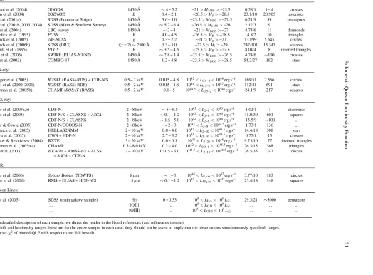
In what follows, we compile a large number of binned QLF measurements in different redshifts ranges, observed wave-bands, and luminosity intervals. Table 1 lists the samples used, with the survey and fields for each, the rest wavelength or band measured, the redshift and luminosity range of the observed quasars, and the number of quasars in the sample. We use the term “quasar” rather loosely throughout, as the traditional MB<−23 cut is not readily applicable to
multi-wavelength observations or obscured sources. Our compi-lation instead attempts to represent all AGN with intrinsic (obscuration-corrected) luminosities above the observational limits at each redshift. This generally extends to the typi-cally adopted ∼1042erg s−1 X-ray luminosity limit (L
bol∼
1010L
⊙), below which confusion with normal star-forming
and starburst galaxies becomes problematic (although re-solved hosts at low redshift extend this to ∼109L
⊙; e.g.,
Hao et al. 2005).
2006b) and find the differences are negligible.
2.1. The SED and Bolometric Corrections
We construct a model “intrinsic” (un-reddened) quasar SED to compare observations in different bands. The tem-plate spectrum initially follows that derived in Marconi et al. (2004) and consists of a broken power law in the optical-UV with αO=−0.44 (Lν ∝ναO) for 1µm< λ <1300 Å (Vanden Berk et al. 2001), and αUV = −1.76 from 1200−
500 Å (Telfer et al. 2002), essentially the modal spectral slopes for optically bright blue quasars (Richards et al. 2006c, appropriate given that this is supposed to be a pre-reddened spectrum). Because a number of slightly different bands have been used in optical quasar surveys (e.g. B, g, i, 1450 Å; see Table 1), we further overlay the template spectrum of Richards et al. (2006c) derived from the optically blue (i.e. un-reddened) subsample onto this broken power-law. Techni-cally, we factor out the best-fit power-law in the given range from the Richards et al. (2006c) spectrum and then multiply our template by the residuals, but this makes little difference compared to adopting the Richards et al. (2006c) spectrum over this range. We do the same with the template spec-trum of Vanden Berk et al. (2001) for optical wavelengths 1µm< λ <1300 Å, if a detailed correction from an observed band to a more “standard” band is needed, but such correc-tions have generally been provided for the QLF measurements in Table 1.
Longwards ofλ >1µm, we adopt the mean spectrum from Richards et al. (2006c), with a typical observed IR “bump” from reprocessing, eventually truncated as a Rayleigh-Jeans tail of blackbody emission (α= 2), and a no-obscuration zero point taken from the optically blue (un-reddened) subsam-ple template spectrum. This gives a 15µm to R-band correc-tion similar to the typically adopted log(L15/LR) = 0.23 (e.g.,
Elvis et al. 1994; Hatziminaoglou et al. 2005; Richards et al. 2006c; Matute et al. 2006; Brown et al. 2006) for optically unobscured (Type 1) quasars.
The X-ray spectrum beyond 0.5 keV is determined by a power-law, with an intrinsic photon index Γ = 1.8 (e.g., George et al. 1998; Perola et al. 2002; Tozzi et al. 2006) and an exponential cutoff at 500 keV. A reflection com-ponent is included following Ueda et al. (2003), generated with the PEXRAV model (Magdziarz & Zdziarski 1995) in the XSPEC package with a reflection solid angle of 2π, inclination cos (i) = 0.5 and solar abundances. The
X-ray spectrum is then renormalized to a given αox ≡
−0.384 log[Lν(2500 Å)/Lν(2 keV)], and the points at 500 Å and 50 Å are connected with a power-law. The value ofαox
depends on luminosity (Wilkes et al. 1994; Green et al. 1995; Vignali et al. 2003; Strateva et al. 2005), and we adopt the most recent determination by Steffen et al. (2006),
αox=−0.107 log(Lν,2500/[erg s−1Hz−1])+1.739, (1)
determined specifically for unobscured (Type 1) quasars. The above equation is derived from the least-squares bisector of the Lν(2500 Å)−Lν(2 keV) relation, since neither luminosity can be properly taken as an “independent” variable – the dif-ference if e.g. Lν(2500 Å) is considered independent is gen-erally small (see e.g. Steffen et al. 2006), but can be of im-portance for the most luminous X-ray AGN (yielding a dif-ference of∼30% in the bolometric correction at L0.5−2 keV∼
1047erg s−1). The baseline for these observations is
suffi-ciently large that this relation has been determined for nearly
10 100
Bolometric Correction (L
BOL
/ L
BAND
)
9 10 11 12 13 14
log(LBOL/LO •)
43 44log(LBOL) [erg s45 46 47 -1
]
B-Band (0.44 µm) Mid-IR (15 µm) Soft X-ray (0.5-2 keV) Hard X-ray (2-10 keV)
FIG. 1.— Bolometric corrections for B-band, mid-IR, soft and hard X-ray
bands, determined in § 2.1 from a number of observations as a function of luminosity and given by the fitting formulae in Equation (2). The lognormal dispersion in the distribution of bolometric corrections at fixed L, given by Equation (3) is shown as the shaded range for each band. The full quasar
template spectrum is available for public download3.
all luminosities of interest in the compiled QLF measure-ments. Recent comparisons between large samples of quasars selected by both optical and X-ray surveys (Risaliti & Elvis 2005) further suggests that this is an intrinsic correlation, not driven by e.g. the dependence of obscuration on lumi-nosity, as does our comparison of bolometric QLFs derived below. There is no evidence for a trend of αox with
red-shift, or for any other trend in spectral shape with redshift (e.g., Elvis et al. 1994; Vanden Berk et al. 2001; Telfer et al. 2002; Vignali et al. 2003; Fan et al. 2003; Steffen et al. 2006; Richards et al. 2006c; Shemmer et al. 2006, but see also Bechtold et al. 2003), so our spectrum depends only on lu-minosity.
Ultimately, the bolometric corrections (with zero attenu-ation) derived can be accurately approximated as a double power-law
L Lband
= c1
L
1010L
⊙ k1
+c2
L
1010L
⊙ k2
, (2)
with (c1,k1,c2,k2) given by (6.25,−0.37,9.00,−0.012)
for Lband = LB, (7.40,−0.37,10.66,−0.014) for
L15µm, (17.87,0.28,10.03,−0.020) for L0.5−2 keV, and
(10.83,0.28,6.08,−0.020) for L2−10 keV. The k1 term is
important when the given portion of the spectrum is not dominant, controlled by the scaling of αox, and the k2≈0
term represents the nearly constant bolometric correction when a given portion of the spectrum dominates the bolo-metric luminosity. Figure 1 shows these corrections as a function of luminosity, which agree broadly with the values in e.g. Richards et al. (2006c) over the luminosity range they consider.
We have generally followed Marconi et al. (2004) in cal-culating this spectrum, with a more detailed treatment of the optical/IR and a more recent determination of αox, but this
level of detail is ultimately not required. The critical de-pendence is that ofαox on luminosity. Adopting the median
Richards et al. (2006c) spectrum and rescaling the spectrum upwards of 0.1 keV according to the observed αox for
to Equation (21) in Marconi et al. (2004) gives a similar re-sult. Ignoring the dependence of bolometric corrections on luminosity altogether, however, is problematic. In the op-tical/UV, it is not as serious, as the bolometric correction
changes by only ∼20% from MB =−23 to −30. However,
over a ∼4 dex interval in L2−10 keV comparable to the usual
observed baselines, the typical hard and soft X-ray bolomet-ric corrections change by more than an order of magnitude (primarily as given by theαox-luminosity relation).
Finally, even accounting for the dependence of spectral shape on luminosity, objects with a given luminosity do not all have identical spectra and bolometric corrections. It is im-portant to account for the dispersion in spectral shapes at a given L. In general, there will be two components, a corre-lated and uncorrecorre-lated dispersion. If, for example, there is a different spectral slope or value ofαox, then the bolometric
correction in certain bands will be larger, but the correction in other bands must be smaller. Also, because the optical/UV contributes a larger fraction of the bolometric luminosity than the X-ray, the resulting dispersion in the B-band bolometric correction from different values of αox will be smaller than
the resulting dispersion in the X-ray bolometric corrections. We estimate these dispersions in the power-law compo-nents of our modeling from the observed distributions, as-suming that they are normally distributed; σαO ≈ 0.125 (Richards et al. 2003, comparing the mean αO in each
ob-served quartile), σΓ = 0.30 (Tozzi et al. 2006), and σαox = 0.075−0.14 (Steffen et al. 2006). Strictly speaking, a larger bolometric correction in one band implies a smaller integrated correction in others, but there are sources of scatter which introduce this effect weakly, such as e.g. variations in line strength in a given band or observational uncertainties in the luminosity in the band. Fitting to the distribution of bolo-metric corrections in Richards et al. (2006c), after account-ing for the luminosity distribution of the sources and corre-lated dispersions above yields a best-fit uncorrecorre-lated disper-sion component∼0.1 dex, consistent with observational esti-mates of the scatter in band luminosities owing to these effects (e.g., Elvis et al. 1994; George et al. 1998; Vanden Berk et al. 2001; Perola et al. 2002; Richards et al. 2003; Hopkins et al. 2004). By fitting to a number of Monte Carlo realizations of the spectra as a function of luminosity given these dispersions, we can quantify the effective dispersion in the bolometric cor-rection in different bands as a function of luminosity
σlog (L/Lbol)=σ1(Lbol/10
9L
⊙)β+σ2 (3)
with (σ1, β, σ2) = (0.08,−0.25,0.060) in the B-band,
(0.07,−0.17,0.086) in the IR (15µm), (0.046,0.10,0.080) in the soft X-ray, and (0.06,0.10,0.08) in the hard X-ray. Here,
σ1 andβ roughly describe the correlated component of the
dispersion,σ2the uncorrelated component. For typical bright
quasars (Lbol∼1013L⊙), this reflects the fact that a significant
(&5%) fraction of quasars in any band can have their bolo-metric luminosities mis-estimated by a factor∼2 or more by a simple bolometric correction (even one that accounts for the luminosity-dependent spectral shape). These dispersions as a function of luminosity are plotted in Figure 1.
2.2. The Observed Column Density Distribution
In order to convert an observed luminosity function to a bolometric luminosity function, we must correct for extinc-tion in the different observed bands, which requires the adop-tion of an observed column density distribuadop-tion. Essentially, the probability of observing a quasar of a given bolometric
luminosity at some observed luminosity in a given band must account for the probability of extinction or attenuation.
We consider three cases. First, our fiducial model adopts the luminosity-dependent observed column density distribu-tion from the hard and soft X-ray observadistribu-tions of Ueda et al. (2003). We also follow Ueda et al. (2003) and include an equal fraction of Compton-thick objects with NH>1024cm−2
to that with NH= 1023−1024cm−2. The evidence for this in
Ueda et al. (2003) is tentative, but it produces good agree-ment with the distribution of Compton-thick column densities subsequently reported by Treister et al. (2004), Mainieri et al. (2005), and Tozzi et al. (2006) and is consistent with upper limits to the obscured fraction from the mid-IR observations of Richards et al. (2006c). Recent very hard X-ray and soft
gamma-ray (∼20−200 keV) Swift BAT and INTEGRAL
ob-servations of local AGN, sensitive even to Compton-thick sources, confirm both a similar Compton-thick fraction and dependence on luminosity (demonstrating also that this trend does not owe to selection effects) (Markwardt et al. 2005; Beckmann et al. 2006a,b; Bassani et al. 2006, but see also
Wang & Jiang 2006). Note that this yields a maximum
Compton-thick fraction of ∼30% (correcting the observed number density in a sample not sensitive to Compton-thick objects by a factor of 1.4), at low luminosity. This does not imply a uniform factor of 1.4 correction to the quasar space density, as the Compton-thick fraction depends on luminosity in the same manner as the entire column density distribution, and the fraction of Compton-thick sources at high luminosity will in general be much smaller.
Alternatively, we consider a constant
(luminosity-independent) column density distribution, again adopting that from Ueda et al. (2003) (fitted to their observations assum-ing no luminosity dependence). As the opposite extreme, we employ the column density distribution determined in La Franca et al. (2005), which depends on both luminosity and redshift. We discuss these models in § 2.3, but find that they are unable to produce a self-consistent set of luminosity functions in the different observed bands.
Given an NHdistribution, we calculate the extinction at
X-ray frequencies using the photoelectric absorption cross sec-tions of Morrison & McCammon (1983) and non-relativistic Compton scattering cross sections. In the optical and mid-IR, we adopt a canonical gas-to-dust ratio (AB/NH)MW =
8.47×10⁻²²cm2and Small Magellanic Cloud-like reddening curve from Pei (1992), which observations suggest is appro-priate for the majority of reddened quasars (Richards et al. 2003; Hopkins et al. 2004; Ellison et al. 2005), although a Milky-Way like reddening curve changes the optical depth by only∼5−10% at the wavelengths of interest (excluding the 2100 Å “bump”).
Given a bolometric QLF and the observed column density distribution, we can then convolve over the distribution of col-umn densities and spectral shapes at each bolometric lumi-nosity L to infer the implied distribution of luminosities that should be observed in a given band. In other words, knowing the probability of some intrinsic spectral shape and interven-ing column density, we determine the probability of observinterven-ing quasars with an intrinsic L at some observed luminosity in the observed band(s).
appro-priate bolometric corrections and then multiplying by some “observable fraction” f (L) to correct for the effects of extinc-tion (and the dispersion in spectral shapes). Fitting to this
f (L) from our full modeling yields a useful function in
com-paring optical, soft X-ray, and hard X-ray observations; more directly applicable than the typically calculated fraction with
NH>1022cm−2. This can be conveniently parameterized as a
power law,
f (L)≡ φ(Li)
φ(L[Li])
= f46
L
1046erg s−1 β
, (4)
where Li is the luminosity in some band, and L is the
cor-responding bolometric luminosity given by the bolometric corrections of Equation (2). This gives values ( f46, β) of
(0.260,0.082) for Li= LB (4400 Å), (0.438,0.068) for Li=
LIR (15µm), (0.609,0.063) for Li = LSX (0.5−2 keV), and
(1.243,0.066) for Li= LHX (2−10 keV). Note that this
“ob-servable fraction” can exceed unity, because the scatter and luminosity dependence of the bolometric corrections signifi-cantly changes the shape of the bright-end QLF in the X-ray bands (see Figure 4 below). These simple rescalings are ro-bust for the B and IR bands, with weak dependence on the shape of the bolometric QLF and dispersion in bolometric corrections, but the effects above make the observable frac-tion in the X-ray bands sensitive to the shape of the QLF; if greater accuracy is required, a more robust fit across a variety of QLF shapes givesβ= 0.035γ2, 0.034γ2for LSX and LHX,
respectively, for an arbitrary bright-end QLF slopeγ2(defined
in § 3.1). We caution that these are crude approximations, but the above equations can be used for rough conversion of ob-served QLFs to bolometric QLFs and vice versa, and for av-erage conversions between bands (multiplying any two such conversions together appropriately).
2.3. Comparison of the Bolometric QLF Under Different Assumptions
Given some model for the quasar spectrum and column density distribution, we can calculate the bolometric QLF from observations in some bands. In detail, we convolve a given bolometric QLF over the distribution of intrinsic spec-tral shapes and column densities, which yields the expected luminosity distribution in some observed band. By integrat-ing, if necessary, over the appropriate redshift and luminos-ity intervals, we can directly compare this to the binned QLF measurements at each frequency, luminosity, and redshift. We minimize theχ2 of this estimate in relation to the observed
QLF in all bands,
χ2≡X φexpected(Lν,z|φbol)−φobs(Lν,z)
∆φobs(Lν,z)
2 , (5)
to determine the best-fit bolometric QLF. Before applying this broadly, we would to test our description of the observed spec-tral shape and column density distributions.
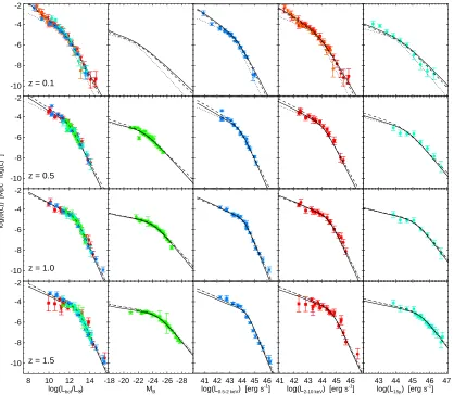
In Figure 2, we show (left panels) the bolometric QLF de-termined in this manner at several redshifts from our full mod-eling. At each redshift, we compare with QLF observations from Table 1 with overlapping redshift intervals. We plot the binned QLF measurements rescaled to bolometric points with respect to the best-fit double power law bolometric QLF at that redshift (see § 3 below). In other words, convolving our best fit bolometric QLF with e.g. the quasar spectrum and col-umn density distribution predicts a number density of quasars
nmdl for a given observed bin. Comparing this to the actual
number observed, nobs, fixes the ratio nobs/nmdl. In Figure 2
we show the agreement with all bands simultaneously by plot-ting nobs/nmdltimes the best-fit bolometric QLF at each
lumi-nosity as the colored points. Given our full SED and obscura-tion model, the inferred bolometric QLF from each observed waveband agrees well. We quantify this directly, showing in each panel the χ2/ν statistic corresponding to the
probabil-ity that all of the observations from the different bands derive from a single (technically double power-law, although this as-sumption only weakly changes theχ2/ν) bolometric QLF.
If, however, we simplify our modeling of observed quasar spectra or column densities, the consistency between the QLF implied from the different wavebands is broken. First, we consider the prediction if all quasars had a single spectral shape by adopting the model spectrum of Elvis et al. (1994), with no dependence on luminosity. The optical, IR, and X-ray observations are no longer consistent with one another, and the χ2/ν at each redshift shown rises by a factor ∼4
to an unacceptably high value. Hard and soft X-ray mea-surements are still consistent, as they are in both cases re-lated by a relatively straightforward power law. These gen-eral conclusions are unchanged regardless of the exact quasar spectrum adopted. In Richards et al. (2006c), mean spec-tra are computed for the entire quasar sample as well as for several sub-samples: the most optically luminous/dim, opti-cally red/blue, and IR luminous/dim halves (divided at the median values log [Lopt/(erg s−1)] = 46.02,∆(g−i) =−0.04,
and log [LIR/(erg s−1)] = 46.04). Figure 3 compares the
bolo-metric QLF as in Figure 2, at z = 1. For clarity, we show only the best-fit double power-law rather than the binned points. Considering the different Richards et al. (2006c) and Elvis et al. (1994) mean spectra, no single quasar spectrum yields a consistent bolometric QLF at all luminosities (i.e. there is no “effective mean” spectral shape). Taking the mean spectrum of the most optically or IR bright quasars, unsur-prisingly, yields a consistent bolometric QLF at the bright end (above the break). The optically and IR dim spectra, on the other hand, are appropriate for lower-luminosity quasars (those near and just below the break), and produce consis-tent bolometric QLFs in this regime. Note that this does
not extend to the lowest luminosities shown, as the “optically
dim” objects in Richards et al. (2006c) are still much brighter (Lbol&1045erg s−1≈3×10¹¹L⊙) than the lowest
luminosi-ties plotted in Figure 3 and probed by X-ray samples. We next examine different assumptions for the column den-sity distribution. In Figure 2, we adopt the full spectral model but consider the luminosity-independent mean column den-sity distribution from Ueda et al. (2003); i.e. a constant ratio of obscured to unobscured AGN∼2 : 1, similar to that found locally (e.g., Risaliti et al. 1999; Hao et al. 2005). Again, the agreement is broken: quasars at low luminosities, where the number of quasars in the Ueda et al. (2003) sample is large, dominate the mean NH distribution, and as a result this
con-stant obscured fraction provides an acceptable (although still less good) fit to the low-luminosity data. However, at high luminosities, the results derived from different wavebands di-verge. The totalχ2/νunambiguously rises (factor∼2) at all
redshifts, with an increasing discrepancy at higher luminosi-ties (factor∼3 increase inχ2/νabove the QLF break). The
-9 -8 -7 -6 -5 -4
z = 1.0 χ2
/ν = 2.1
Luminosity-Dependent BC/NH
-9 -8 -7 -6 -5 -4
z = 1.5 χ2
/ν = 2.1
-9 -8 -7 -6 -5 -4
z = 2.0 χ2
/ν = 1.0
11 12 13 14 15
-9 -8 -7 -6 -5 -4
z = 3.0 χ2
/ν = 1.4
log(
φ
(L)) [Mpc
-3 log(L) -1 ]
χ2
/ν = 8.5 Fixed BC
χ2
/ν = 9.2
χ2
/ν = 6.1
11 12 13 14 15
χ2
/ν = 4.3
log(Lbol/LO •)
χ2
/ν = 4.5 Fixed NH
χ2
/ν = 4.4
χ2
/ν = 4.7
11 12 13 14 15
χ2
/ν = 2.2
χ2
/ν = 3.8
Redshift-Dependent NH
χ2
/ν = 5.5
χ2
/ν = 5.7
11 12 13 14 15
χ2
/ν = 6.6
FIG. 2.— The bolometric QLF from the observations in Table 1 at various wavebands (optical: green, soft X-ray: blue, hard X-ray: red, IR: cyan; see
Table 1 for the plotting symbols). For ease of comparison, the points in the different bands are rescaled as described in the text to indicate the bolometric QLF implied by each set of measurements. Left panels show the bolometric QLF adopting our full (luminosity-dependent) bolometric corrections and column density distributions (see also Ueda et al. 2003; Marconi et al. 2004; La Franca et al. 2005), at several redshifts (as labeled). Center-left shows the result with the full column distribution, but adopting the constant bolometric corrections of Elvis et al. (1994). Center-right uses the full bolometric corrections, but a luminosity-independent column density distribution (obscured fraction). Right uses the full bolometric corrections and a strongly redshift-dependent column
density distribution from La Franca et al. (2005). Each panel shows the reducedχ2for the assumption that the data yield a consistent bolometric QLF at each
redshift. The latter three assumptions do not yield a consistent bolometric QLF at each redshift, unlike for the observationally derived luminosity-dependent bolometric corrections and column density distributions.
Finally, we adopt a column density distribution which evolves strongly with redshift (and luminosity). Specifically, we adopt the fit from La Franca et al. (2005) to the NH
dis-tribution with maximal redshift evolution, similar to the red-shift evolution implied by the column density distributions in Tozzi et al. (2006) (fitted assuming maximal redshift depen-dence and no luminosity dependepen-dence), and similar to the red-shift evolution of obscured fractions implied by some X-ray background synthesis models (e.g., Comastri et al. 1995; Gilli et al. 1999; but see also Treister & Urry 2005). The resulting bolometric QLF is shown in the right panels of Figure 2.
This fit is reasonable at low and moderate redshifts z.1 (unsurprisingly, where the observed samples are best
con-strained). Extrapolated to higher redshifts, the consistency between different bands breaks down, increasingχ2/νby an
-10 -8 -6 -4
Full Corrections R06: All R06: Blue
-10 -8 -6 -4
R06: Red
log(
φ
(L)) [Mpc
-3 log
10
(L)
-1 ]
R06: Optically Bright R06: Optically Dim
8 10 12 14
-10 -8 -6 -4
R06: IR Bright
8 10 12 14
R06: IR Dim
log(Lbol/LO •)
8 10 12 14
Elvis (1994)
FIG. 3.— Comparison of the best-fit bolometric QLFs to the observations in Figure 2 at z∼1, fitted independently to the optical (green), soft X-ray (blue),
hard X-ray (red), and IR (cyan) data sets. Upper left panel shows the result using our full (luminosity-dependent) bolometric corrections, with the black line the bolometric QLF from fitting to the data at all wavelengths simultaneously (reproduced as the dashed black line in the other panels), subsequent panels adopt constant (luminosity-independent) corrections from Richards et al. (2006c) based on the mean spectrum of the complete (all), blue, red, optically bright, optically dim, IR bright, and IR dim sub-samples considered therein. Lower right panel adopts the Elvis et al. (1994) mean spectrum. Accounting for the dependence of spectral shape on luminosity yields a consistent bolometric QLF across all frequencies and luminosities, whereas considering a single mean spectrum is generally appropriate only for narrow luminosity and color intervals.
moderate redshifts.
Likewise, although not shown in Figure 2, we find no evi-dence for any depenevi-dence of bolometric corrections on red-shift, in agreement with a number of direct measurements of quasar SEDs (e.g., Elvis et al. 1994; Vanden Berk et al. 2001; Telfer et al. 2002; Vignali et al. 2003; Fan et al. 2003; Steffen et al. 2006; Richards et al. 2006c; Shemmer et al. 2006). If the variation of e.g.αox were primarily a redshift
as opposed to luminosity dependence, or if there were e.g. a strong dependence of X-ray photon index on redshift as sug-gested by Kuhn et al. (2001) and Bechtold et al. (2003), then our inferred bolometric QLFs from different bands would di-verge with redshift. Instead, they appear to be self-consistent given the redshift-independent spectral model at all z = 0−6. Given the limitations of present data, however, it is still possi-ble that less well-constrained portions of the spectrum evolve differently. For example, the IR SED could, in principle, evolve differently with luminosity or redshift from the opti-cal SED (but see Jiang et al. 2006b, who find similar near-IR SEDs at high redshift), and Maiolino et al. (2004) have sug-gested that extinction curves may evolve at z&4−5 (although their proposed extinction curves change the optical depth at the wavelengths of interest by.10%). There is no strong evidence for such additional evolution in the samples we con-sider, but these caveats should be considered in any extrapo-lation of our fitting to less well-sampled frequencies and red-shifts.
2.4. The Relation of Bolometric to Observed QLFs
We briefly examine the relation between the shape of the bolometric QLF and the observed QLF at different frequen-cies. Figure 4 shows the fit to the bolometric QLF from Fig-ure 2, at z∼1, and the resulting observed QLF in different bands. Although our fitting considers all observations in the bands given in Table 1, we have renormalized all optical ob-servations to the B-band for plotting purposes (likewise for the other bands). We plot all observations in the same units (B-band and 15µm showνLν) for the sake of direct compari-son.
evaluat-ing e.g. the UV contributions of quasars, is affected at the faint and bright ends by obscuration and changing bolometric corrections, respectively.
2.5. The Contribution of Quasar Host Galaxy Light
We have so far ignored the contribution of quasar host galaxies to their observed luminosities. Observed luminos-ity functions, however, do not generally remove this host contamination. In the X-ray bands, this is not of course expected to be a serious concern, and in the emission-line luminosity functions of Hao et al. (2005) we consider their more conservative AGN cut which should eliminate much of the contamination from star-forming nuclear regions in the hosts. However, this contribution may still be problematic at optical and IR wavelengths. If we knew the black hole masses of quasars in the observed QLFs, it would be straight-forward to at least estimate an average host contribution or bias, as there is a well-established correlation between black hole mass and host galaxy optical luminosity (or mass) (e.g., Kormendy & Richstone 1995). Lacking this information, we must adopt some estimate of the observed quasar Eddington ratio (L/LEdd) distribution to convert from a bolometric
lumi-nosity to black hole mass and corresponding host lumilumi-nosity. In Figure 5, we consider several simple, representative cases to estimate the possible effects of our neglecting host lu-minosities. We compare the B-band QLF neglecting host light (our fiducial model) and alternatively, assuming all quasars are radiating at the Eddington luminosity. This gives a black hole mass for each L, and we use the black hole mass-host B-band luminosity relationship from Marconi & Hunt (2003) to determine the corresponding host contribution (see also Vanden Berk et al. 2006, who measure a similar L/LEdd
-dependent relation directly in AGN). The quasar luminosi-ties are corrected and attenuated as before, and then the (un-attenuated) host luminosity is added.
Strictly speaking, this is not necessarily self-consistent, as the observational calibrations of bolometric corrections do not necessarily remove host galaxy contributions. However, our construction of the intrinsic quasar SED should effectively ex-clude host contributions (compare e.g. Richards et al. (2006c) who explicitly remove a rough lower limit to the host contri-bution), so long as there is not a substantial host contribution at∼2500 Å which would significantly affect the determina-tion ofαox(although this is not expected at these frequencies,
and the relation in Steffen et al. (2006) is calibrated from only Type 1 AGN). In any case, these effects are second-order to those shown in Figure 5.
We also consider the case where all quasars radiate at an Eddington ratio L/LEdd= 0.3 and L/LEdd= 0.1. As an
alterna-tive simplification, we consider the case if the QLF is a pure Eddington ratio sequence with L/LEdd= L/L∗(L∗is the fitted
QLF break luminosity). It makes no difference if we allow
L/LEdd>1 or fix the maximum L/LEdd= 1, as the host
contri-bution is minimal in either case. We show this for the B-band, but the effects in the mid-IR are similar (given e.g. the typi-cal early-type spectrum of Fioc & Rocca-Volmerange (1997); effects are also similar for other host types).
Figure 5 demonstrates that including quasar host galaxy minosities should be a small effect, except at the lowest lu-minosities MB&−23 (bolometric L.1012L⊙). This is
un-surprising, as at bright observed MB, obscuration is small
and Eddington ratios are expected to be high. In general, this implies a negligible impact on our subsequent calcula-tions, as the deepest optical observations only just probe the
range in which host luminosity contamination becomes sig-nificant (the larger baseline at low luminosities comes from hard X-ray observations, which do observe significant num-bers of optically normal galaxies hosting low-luminosity X-ray AGN, e.g. Barger et al. 2005). At higher redshift, flux lim-ited samples are further removed from these luminosities, and Eddington ratios are expected to be uniformly high (at least in optically-selected samples, e.g. McLure & Dunlop 2004). Moreover, observations of the relation between black hole mass and host luminosity at high redshift, albeit considerably uncertain, suggest that host luminosities either remain con-stant or decrease at a given MBH(e.g., Peng et al. 2006).
However, this strongly cautions the interpretation of deeper optical, near- or mid-IR surveys, especially at low redshifts
z.0.5, where Eddington ratios may well be low (.0.1). If such surveys seek to probe luminosities .1012L
⊙,
care-ful consideration of the contribution from quasar hosts is nec-essary to determine the actual quasar contribution at low lu-minosities. For example, Figure 5 demonstrates that the ob-served faint-end QLF slope in these bands can be significantly biased by host contamination at magnitudes lower than those currently probed, in a manner sensitive to the Eddington ra-tio or black hole mass distribura-tion. These effects will be even more pronounced in the near-IR, as the ratio of host to quasar luminosity in unobscured objects has a typical maximum at
ν∼1.6µm (see e.g. Figure 11 of Richards et al. 2006c).
3. THE BOLOMETRIC QLF
3.1. The Bolometric QLF at Specific Redshifts
We combine the binned QLF measurements to examine the QLF “at” a single redshift. Of course, the observations are not made over identical redshift intervals, so we re-normalize each to the same redshift (as nobs/nmdl) with the best-fit
ana-lytic QLF fit from the same (or appropriate companion) paper. This introduces some additional model dependence, so these fits should be considered as heuristic, but they will inform our subsequent choice of functional forms for more properly fit-ting to the redshift dependence of the bolometric QLF.
We follow standard practice and fit the QLF to a double power law
φ(L)≡ dΦ
d log(L)=
φ∗
(L/L∗)γ1+(L/L∗)γ2
, (6)
with normalizationφ∗, break luminosity L∗, faint-end slope γ1, and bright-end slope γ2. Note that conventions for the
double power law are often different in optical and X-ray anal-yses; for optical QLFs typically the double power law is de-fined in terms of (e.g., Peterson 1997; Croom et al. 2004)
dΦ
dL =
φ′∗/L ∗
(L/L∗)−α+(L/L∗)−β
, (7)
or per unit absolute magnitude
dΦ
dM=
φ′′ ∗
100.4 (α+1) (M−M∗)+100.4 (β+1) (M−M∗),
(8)
which in our notation givesα=−(γ1+1),β=−(γ2+1),φ′∗= φ∗/ln 10, andφ′′
∗= 0.4φ∗.
-9 -8 -7 -6 -5 -4
log(
φ
(L)) [Mpc
-3 log(L) -1 ]
Optical (B-band) Soft X-ray (0.5-2 keV)
42 43 44 45 46 47
-9 -8 -7 -6 -5 -4
log(L) [erg s-1] Hard X-ray (2-10 keV)
42 43 44 45 46 47
Mid-IR (15 µ)
FIG. 4.— The best-fit bolometric QLF at z∼1 (black lines), with the resulting observed QLF in each of several bands: optical (green), soft X-ray (blue), hard
X-ray (red), and IR (cyan). Each corresponding panel plots the compiled observations in Table 1 for the appropriate redshift and frequency (points). Symbols denote the parent sample as given in Table 1. The observations at each band are consistently produced from a single bolometric QLF, and together provide strong constraints on the QLF shape. Different wavebands accurately represent different aspects of the bolometric QLF shape. With only a weakly L-dependent bolometric correction but significant effects of obscuration, the optical QLF faithfully traces the bolometric bright end shape, but is flatter at faint L. Hard X-rays, conversely, are weakly affected by obscuration but can have a strongly luminosity-dependent bolometric correction, reproducing the faint end shape but being steeper at bright L. The IR QLF better follows the bolometric shape, but is currently least well-constrained.
observed spectral and NHdistributions is employed.
Further-more, the combination of this number of observations pro-vides a large luminosity and redshift baseline, sampling the the faint end, break, and bright-end slope to redshifts z∼4−5. We plot the best-fit parameters from these fits at a number of redshifts in Figure 8 (error bars show formal 1σ uncertain-ties from the fits), and list them at several redshifts in Table 2. The normalizationφ∗is roughly constant, while the break lu-minosity (which is quite tightly constrained for most of the redshift range) evolves by∼2 orders of magnitude. Note that the points whereφ∗ appears to deviate from being constant also have discrepant L∗values — the degeneracy between the
two is such that the value ofφ∗is consistent with being con-stant at all z for smooth evolution in L∗. There is an indication
of evolution in both the faint-end and bright-end slopes, which we discuss below. The integrated bolometric luminosity den-sity is well constrained, with the largest uncertainties only
∼0.15 dex. We determine the luminosity density by integrat-ing the best-fit luminosity function to L = 0. At most redshifts
z&0.5 the faint-end slope is relatively shallow, and choosing instead a cutoff at e.g. L = 108−109L⊙changes the integrated
luminosity density by.10%. At the lowest redshifts, how-ever, the faint-end slope is steep, and at z = 0 where this is
most pronounced, the luminosity density is ∼15% lower if we truncate at L = 108L⊙(∼25% lower for L = 109L⊙). This
sensitivity to the steep faint-end slope at low-z is the reason for the relatively large uncertainty in the luminosity density at low redshift. At high-z the uncertainty owes to the limited amount of data. In any case there is a well-defined peak in the luminosity density at z = 2.154±0.052 (formal error from fit; we expect a systematic error±0.15 from choices in sampling and binning the observations), well outside the range where either of these systematic concerns is problematic.
3.2. Analytic Fits as a Function of Redshift
We characterize the QLF as a function of redshift by adopt-ing a standard pure luminosity evolution (PLE) model, where the bolometric QLF is a double power law at all z, with con-stantγ1,γ2, andφ∗, but an evolving L∗. We allow L∗to evolve
as a cubic polynomial in redshift,
log L∗= (log L∗)0+kL,1ξ+kL,2ξ2+kL,3ξ3, (9)
where
ξ= log 1+z 1+zref
. (10)
Here, kL,1, kL,2, and kL,3 are free parameters, and we set
-20 -22 -24 -26 -28 MB
-8 -7 -6 -5 -4
log(
φ
(M
B
)) [ Mpc
-3 log(L) -1 ]
No Host L / LEdd = 1.0
L / LEdd = 0.3 L / LEdd = 0.1
L / LEdd∼ L / L∗
FIG. 5.— The observed B-band QLF (points) at z∼1, and that determined
from the best-fit bolometric QLF in Figure 4 (solid line) ignoring contribu-tions to the observed luminosity from quasar host galaxies. Also shown is the B-band QLF determined from the same bolometric QLF, but including the ex-pected host galaxy contribution to the observed luminosities (normalized for a given Eddington ratio with the observed relation between black hole mass and host galaxy B-band luminosity from Marconi & Hunt (2003)), assuming all quasars have constant L/LEdd= 1.0, 0.3, 0.1 (dot-dashed, long-dashed,
dotted lines, respectively), or assuming L/LEdd= L/L∗(short dashed line; L∗
is the QLF break luminosity). Host galaxy contributions should be negligible at most luminosities and redshifts for the observed bands we consider, but will be important for future optical, near- and mid-IR surveys which probe
fainter luminosities L.1012L
⊙(MB&−23).
The cubic term is demanded by the data (∆χ2∼600 on its
addition), but higher order terms inξare not (∆χ2.1). Since
this model includes the evolution with redshift, we can simul-taneously fit to all the data sets in Table 1, each over the ap-propriate redshift intervals of the observed samples.
The best-fit PLE model parameters are given in Table 3 and plotted as a function of redshift in Figure 8, and the resulting QLF is shown in Figures 6 & 7. Although this provides a rea-sonable lowest-order approximation to the data, it fails at the faint end, underpredicting the abundance of low-luminosity sources at z.0.3 and overpredicting it at z&2, and the fit is poor at z&5 with much too steep a bright end slope. Over the entire data set, the fit is unacceptable, withχ2≈1924 for
ν= 510 degrees of freedom. A pure density evolution (PDE) model fares even worse, withχ2/ν= 3255/510 (although for
completeness we provide the best-fit PDE parameters in Ta-ble 4), unsurprising given that nearly every observed data set which resolves the break in the QLF favors the PLE form (e.g., Boyle et al. 2000; Miyaji et al. 2000; Ueda et al. 2003; Croom et al. 2004; Richards et al. 2005).
As discussed in § 1, many recent studies have found ev-idence for evolution in the faint end beyond that predicted by PLE, with the density of lower-luminosity sources peak-ing at lower redshift than the density of higher-luminosity sources, and have fit this trend with a luminosity-dependent density evolution (LDDE) model (Schmidt & Green 1983), while high-redshift samples have suggested evolution in the bright-end QLF shape, confirmed robustly as a flattening in
γ2 for the first time in a homogeneous sample by the SDSS
(Richards et al. 2006c). We wish to incorporate this additional evolution into our model.
For comparison with these results and future X-ray surveys, we fit to an LDDE form allowing maximal flexibility of the parameters,
φ(L,z) =φ(L,0) ed(L,z) (11)
= φ∗
(L/L∗)γ1+(L/L∗)γ2
ed(L,z). (12)
The density function edis given by
ed(L,z) =
(1+z)p1 (z≤zc)
(1+zc)p1[(1+z)/(1+zc)]p2 (z>zc)
(13)
with
zc(L) =
zc,0(L/Lc)α (L≤Lc)
zc,0 (L>Lc) (14)
and
p1(L) = p146+β1[log(L/1046erg s−1)] (15)
p2(L) = p246+β2[log(L/1046erg s−1)]. (16)
Note that some authors (e.g., Hasinger et al. 2005) adopt an alternative normalization convention in terms of A44≡φ(L =
1044erg s−1,z = z
c) and zc,44 ≡zc(L = 1044erg s−1), but these
choices are not particularly convenient for the bolometric QLF. The 11 free parameters in this fit are then L∗,φ∗,γ1,
γ2, zc,0, Lc, α, p146, p246,β1,β2. Their best-fit values are
given in Table 4.
The LDDE form can effectively describe evolution in the faint-end QLF slope, but it does not allow for evolution in the bright-end slope. It also has a tendency to introduce a “second break” in the faint end of the QLF (i.e. if the faint end flattens there is often some L below which it rises steeply again), for which we see no evidence. Ultimately, the improvement over the PLE fit is highly significant, withχ2/ν= 1389/507, but
there is still room for substantial improvement.
Therefore, we instead consider the PLE form above, but allow both the bright- and faint-end slopes to evolve with red-shift. For the faint-end slope, using the fitted points at each
z to inform our choice of functional form, we modelγ1as a
power-law in redshift,
γ1 = (γ1)0×10kγ1ξ (17) = (γ1)0
1+z
1+zref
kγ1
, (18)
where again zref= 2 is fixed. Allowing this dependence (while
still holdingγ2constant) significantly improves the quality of
the fit relative to the PLE model, reducingχ2 by
∆χ2≈500
with the addition of one parameter, toχ2/ν= 1422/510. The
values for this fit are given in Table 3. There is no evidence for higher-order terms (∆χ2.1 for the addition of a
second-order power in ξ). We have also tested different functional forms, and do not find any which provide a significantly better fit. This choice also has the advantage that it extrapolates to a flatγ1→0 (as opposed to a negative, likely unphysical) slope
at high redshift.
Parameterizing evolution in the bright-end slope is more difficult. There appears to be evidence for a steepening of the bright-end slope (increase inγ2) from z∼0 to z∼1.5,
then a flattening with redshift. We find the best results for a double-power law of the form
γ2= (γ2)0×2 h
10kγ2,1ξ+10kγ2,2ξi−
1
(19)
= 2 (γ2)0
1+z
1+zref
kγ2,1 +
1+z
1+zref
kγ2,2. (20)
Here, kγ2,1describes the rise ofγ2with z at low redshift, and
fac--10 -8 -6 -4 -2
z = 0.1
-10 -8 -6 -4 -2
z = 0.5
log(
φ
(L)) [Mpc
-3 log(L) -1]
-10 -8 -6 -4 -2
z = 1.0
8 10 12 14 log(Lbol/LO •)
-10 -8 -6 -4 -2
z = 1.5
-18 -20 -22 -24 -26 -28 MB
41 42 43 44 45 46 log(L0.5-2 keV) [erg s-1
]
41 42 43 44 45 46 log(L2-10 keV) [erg s-1
]
43 44 45 46 47 log(L15µ) [erg s-1
]
FIG. 6.— The best-fit bolometric QLF at each of several redshifts (left panels; shown as nmdl/nobs), and the corresponding observed QLF in B-band (center-left;
green), soft X-rays (0.5−2 keV) (center; blue), hard X-rays (2−10 keV) (center-right; red), and mid-IR (15µm) (right; cyan). Rather than add a series of panels
for a single data set, the emission-line luminosity functions of Hao et al. (2005) are shown (orange) in the z = 0.1 hard X-ray panel (rescaled by nobs/nmdl, but
equivalently directly converted to hard X-ray luminosities following Heckman et al. 2005). Lines show the best-fit evolving double power-law model to all redshifts (solid), the best-fit model at the given redshift (dashed), and the best-fit PLE model (dotted). Points shown are the compiled observations from Table 1, with the plotting symbols for each observed sample listed therein.
tor of 2 is inserted such that if kγ2,1 = kγ2,2= 0, the
result-ing γ2= (γ2)0. The best-fit parameters, fixing γ1 or
allow-ing both slopes to evolve simultaneously, are given in Ta-ble 3. We find that kγ2,1 is non-zero at high formal
signifi-cance, but cannot say whether this steepening up to z∼1.5 is “real” in any robust sense; however, including this pa-rameter does significantly improve the accuracy of our fit-ting function in represenfit-ting the binned data. The flatten-ing at high redshifts is more significant (∼7σ). Including these two parameters greatly improves the quality of the fit by
∆χ2≈600, givingχ2/ν= 1312/509 for a fit with constantγ 1
orχ2/ν= 1007/508 for a simultaneous fit including evolution
inγ1andγ2. Again, there is no evidence for terms describing
further evolution. Although our final best fit does not cross this limit until the highest redshifts, we also formally enforce a lower limitγ2≥1.3 (to prevent an unphysical divergence in
the luminosity density).
The best-fit parameters as a function of redshift (allowing all free parameters to vary) are plotted in Figure 8. There is a slight offset between the L∗ andφ∗ of this fit and that
fitted at specific redshifts, but this owes to their covariance.
This can be seen in the bolometric luminosity density, which accurately traces the fit predictions (note that the PLE model significantly overpredicts the luminosity density at z>2, as it overpredicts the number of faint sources). Our restriction
γ2≥1.3 is important in extrapolating beyond z∼5 to prevent
a divergence in the number and luminosity density of bright sources. We also plot the predicted number density of quasars with MB<−27 as a function of redshift, which agrees with the
direct observations (expected, but nevertheless a reassuring consistency check).
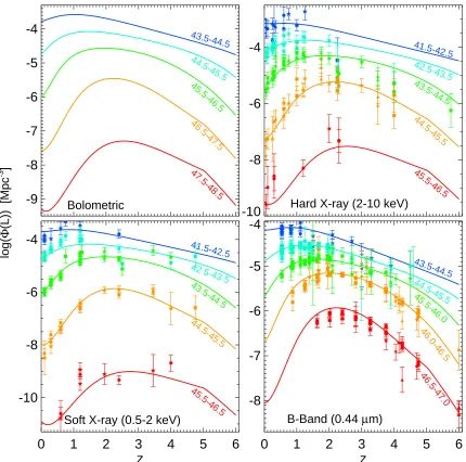
Figure 9 plots the number density of quasars integrated over various luminosity intervals, in various bands as a function of redshift, from the best-fit model and the compiled observa-tions in Table 1. Although this information is contained in Figures 6 and 7, Figure 9 nicely illustrates an essential trend captured by the LDDE or evolving double power-law forms, namely that the density of lower-luminosity sources peaks at lower redshift than that of higher-luminosity sources. The trend is evident in all bands we consider.
[image:12.612.102.520.69.433.2]-10 -8 -6 -4 -2
z = 2.0
-10 -8 -6 -4 -2
z = 3.0
log(
φ
(L)) [Mpc
-3 log(L) -1]
-10 -8 -6 -4 -2
z = 4.0
8 10 12 14 log(Lbol/LO •)
-10 -8 -6 -4 -2
z = 5.0
-18 -20 -22 -24 -26 -28 MB
41 42 43 44 45 46 log(L0.5-2 keV) [erg s-1
]
41 42 43 44 45 46 log(L2-10 keV) [erg s-1
]
43 44 45 46 47 log(L15µ) [erg s-1
]
FIG. 7.— As Figure 6, but at higher redshifts, as labeled.
the double power-law of Equation (6), we consider a modified Schechter function
φ(L) =φ∗(L/L∗)−γ1exp n
−L
L∗ γ2o
. (21)
We have also, for example, adopted polynomials of arbitrar-ily high order (although the fits typically do not improve be-yond fourth order). In either case, the fit is quite similar at most luminosities (with similarχ2/ν), implying that there is
no dramatic shape dependence which we have not captured. However, such a fit does exhibit smoother curvature rather than a sharp break at L∗, evidence for which has been seen in
some optical samples (e.g., Wolf et al. 2003; Richards et al. 2005). At the highest luminosities (&1 dex above L∗,
typi-cally Lbol&1014L⊙) the implied number of quasars is an
or-der of magnitude lower for these parameterizations than for the double power law prediction, and falls much more rapidly. The resulting observed luminosity functions are more sensi-tive to the estimated dispersion in bolometric corrections, but in either case the highest luminosity soft and hard X-ray ob-jects in Figures 6 & 7 are substantially affected by quasars shifting into slightly larger bins of soft or hard X-ray lumi-nosity owing to different spectral shapes (e.g. the scatter in
αox). It is important to account for this effect when
attempt-ing to infer the number density of the most massive black
holes and most luminous quasars, as a naive extrapolation of the median bolometric corrections applied to the most X-ray bright quasars implies extreme (and potentially unphysical) bolometric luminosities&1015L⊙(i.e. a&3×10¹⁰M⊙black
hole at the Eddington rate). Multiwavelength observations of these particular objects and further study from large area surveys which do not have to bin in widely spaced luminos-ity intervals will be critical in breaking the degeneracies be-tween these fits to the intrinsic bolometric QLF and the double power-law form.
We are unable to find any further dependences which sig-nificantly improve the best-fit QLF. Allowing the parameters describing the observed column density distribution and spec-tral shape, and their respective luminosity dependence, to vary simultaneously, yields only marginal improvement. It appears that the remaining scatter in the data does not mostly owe to a failure to capture some remaining dependence. In Table 1 we list theχ2/ν for each sample with respect to the best-fit
full model of the evolution of the QLF in Table 3. The agree-ment with most samples is good, and the largest, most well-constrained samples (with small typical≪0.1 dex errorbars) give χ2/ν .3, in each case comparable to or smaller than
the reducedχ2found by the respective authors in fits to those
individual data sets. To the extent that the functional forms
0 1 2 3 4 5 6 z
-0.2 0.0 0.2 0.4 0.6 0.8 1.0
Faint-End Slope
γ1
0 1 2 3 4 5 6
z 1.0
1.5 2.0 2.5
Bright-End Slope
γ2
0 1 2 3 4 5 6
z -5.5
-5.0 -4.5 -4.0
Normalization log(
φ∗
) [Mpc
-3]
0 1 2 3 4 5 6
z 11.5
12.0 12.5 13.0
Break Luminosity log(L
∗
) [L
O
•
]
0 1 2 3 4 5 6
z 6.5
7.0 7.5 8.0
Luminosity Density log(j
bol
) [L
O
•
Mpc
-3]
0 1 2 3 4 5 6
z -9.5
-9.0 -8.5 -8.0 -7.5 -7.0
log[
Φ
(z, M
B
< -27) ] [Mpc
-3]
FIG. 8.— The best-fit QLF double-power law parameters as a function of redshift. Points show the best-fit values to data at each redshift, dotted lines the best-fit
PLE model, and solid lines the best-fit full model (with cyan shaded range showing the 1σuncertainty). Open diamonds inγ2(z) show the bright-end slope fits
from Richards et al. (2006b). Although PLE is appropriate for a lowest-order fit, both the bright and faint-end slopes evolve with redshift to high significance
(>6σ). Lower right shows the predicted number density of bright optical (MB<−27) quasars from the full fit (solid), compared to that observed in Croom et al.
(2004) (square), Richards et al. (2006b) (diamonds and dashed line), and Fan et al. (2004) (circle).
this level, we would not expect to do better in the combined sample.
There will also be some unavoidable variance introduced owing to systematic variations between independent data sets. Various observational calibrations, the model dependences in-herent in calculating a binned QLF, and most of all cosmic variance will all contribute to sample-to-sample differences. In fact, we find that allowing for even a small ∼0.05 dex (10−15%) systematic normalization variance between sam-ples, most of the remaining scatter is accounted for, with a best-fit model improvement∆χ2∼500. We provide the
val-ues of this fit in Table 3, but caution that we have increased the sample-to-sample variance by this amount uniformly, when in fact systematic effects such as cosmic variance will be smaller for large surveys such as the SDSS and 2dF than for the small deep fields of Chandra and XMM. Consequently, this under-weights some of the most well-constrained observations, and the fit results should be considered to be heuristic.
4. THE BUILDUP OF THE BLACK HOLE POPULATION
4.1. Model-Dependent Quantities
We can gain further insight into the evolution of the QLF, albeit at the cost of some model dependence, by de-convolving the observed quasar luminosity function with a theoretical model for the quasar light curve or lifetime. This method is well-established (e.g., Salucci et al. 1999; Yu & Tremaine 2002; Marconi et al. 2004; Shankar et al. 2004; Yu & Lu 2004), but most studies adopt simplified “toy” light curves with accretion at a constant (fitted) absolute rate or Eddington ratio and fitted lifetimes and duty cycles. We
instead follow Hopkins et al. (2006b), who derive physically motivated quasar light curves from simulations of merging galaxies that include black hole growth (e.g. Springel et al. 2005b) and which are consistent with a large range of obser-vational constraints that cannot be reproduced by idealized models. This also removes the various fitting degeneracies – for a given bolometric QLF, the quasar light curves deter-mined in simulations yield a unique black hole mass function, cosmic X-ray background spectrum, and self-consistent black hole and host galaxy properties.
Given a consistent model of the quasar lifetime/lightcurve, the observed bolometric QLF is given by the convolution of the rate of quasar formation or “triggering” with the differen-tial quasar lifetime,
φ(L) =
Z
˙
φ(MBH)
dt
d log L(L|MBH) d log MBH (22) where
˙
φ(MBH) =
dΦ(MBH,t)
d log MBHdt
(23)
is the rate of formation of black holes of a relic mass MBH
at cosmic time t. Since dt/d log L is completely determined in the simulations and analytical models of Hopkins et al. (2006a,b), we can fit toφ˙(MBH) in the same manner that we
have fittedφ(L).
We assume a double power-law form forφ˙(MBH) at all z,
˙
φ(MBH) =
˙
φ∗
(MBH/M∗)η1+(MBH/M∗)η2
-9
-8
-7
-6
-5
-4
43.5-44.544.5-45.5
45.5-46.5
46.5-47.5
47.5-48.5
Bolometric
-10
-8
-6
-4
41.5-42.542.5-43.5
43.5-44.5
44.5-45.5
45.5-46.5
Hard X-ray (2-10 keV)
0
1
2
3
4
5
6
z
-10
-8
-6
-4
log(
Φ
(L)) [Mpc
-3
]
41.5-42.5
42.5-43.5
43.5-44.5
44.5-45.5
45.5-46.5
Soft X-ray (0.5-2 keV)
0
1
2
3
4
5
6
z
-8
-7
-6
-5
-4
43.5-44.5
44.5-45.5 45.5-46.0
46.0-46.5
46.5-47.0
B-Band (0.44
µ
m)
FIG. 9.— Total number density of quasars in various luminosity intervals (in log (Lband/[erg s−1]) as labeled) as a function of redshift, from the best-fit evolving
double-power law model (lines) and the compiled observations in Table 1 (points of corresponding colors, symbols for each sample listed therein) in bolometric
luminosity, B-band, soft X-rays (0.5−2 keV), and hard X-rays (2−10 keV). The trend that the density of lower-luminosity AGN peaks at lower redshift is manifest
in all bands.
with normalizationφ∗˙ , break M∗, and faint-end and
bright-end slopesη1 andη2, respectively. We determine an
analyti-cal fit toφ˙(MBH,z) in the same manner asφ(L,z). We allow
log M∗ to vary as a cubic inξjust as L∗, and allow the
high-mass slopeη2to vary just asγ2, as well. There is no evidence
for evolution of the low-mass slope η1. In this formulation
there is evidence for evolution inφ∗˙ above z∼2, so we fix it to a constant below zref≡2, and allow it to evolve as a
power-law above zref,
˙
φ∗(z) =
(φ∗˙ )0 (z≤zref)
(φ∗˙ )0[(1+z)/(1+zref)]kφ˙ (z>zref).
(25)
In Figure 10, we plot the best-fit normalizationφ∗˙ and break (characteristic mass in formation) M∗ as a function of
red-shift. At high redshifts, objects build up rapidly, until z∼2, after which the rate of merger/black hole growth “events” flat-tens, and activity ceases in the most massive systems and
rapidly moves to less massive objects at lower redshifts, per-haps driven by feedback mechanisms quenching activity in the higher-mass systems. Given the adopted lifetime mod-els, the observed faint-end φ(L) slope γ1 is dominated by
sources with L≪LEdd(MBH) and is determined by the quasar
lifetime as a function of MBH. Figure 10 shows the
pre-dictedγ1(z) from the quasar lifetime model given the best-fit
˙
φ(MBH) at each z, compared to the direct fits from Figure 8;
the agreement is good despite η1 being nearly constant and
much flatterη1≈0.0−0.2 at all redshifts (see also Figure 3 of
Hopkins et al. (2006a)).
4.2. Integrated Quantities
If all black holes accrete with some constant radiative effi-ciencyǫr,
[image:15.612.93.523.66.492.2]