This is a repository copy of
Health Economic Assessment of Public Health Strategies for
Alcohol Harm Reduction: The Sheffield Alcohol Policy Model Framework
.
White Rose Research Online URL for this paper:
http://eprints.whiterose.ac.uk/43755/
Article:
Brennan, A., Meier, P., Purshouse, R. et al. (3 more authors) (2012) Health Economic
Assessment of Public Health Strategies for Alcohol Harm Reduction: The Sheffield Alcohol
Policy Model Framework. HEDS Discussion Paper, 12/03. (Unpublished)
eprints@whiterose.ac.uk https://eprints.whiterose.ac.uk/ Reuse
Unless indicated otherwise, fulltext items are protected by copyright with all rights reserved. The copyright exception in section 29 of the Copyright, Designs and Patents Act 1988 allows the making of a single copy solely for the purpose of non-commercial research or private study within the limits of fair dealing. The publisher or other rights-holder may allow further reproduction and re-use of this version - refer to the White Rose Research Online record for this item. Where records identify the publisher as the copyright holder, users can verify any specific terms of use on the publisher’s website.
Takedown
If you consider content in White Rose Research Online to be in breach of UK law, please notify us by
HEDS Discussion Paper
No. 12/03
Health Economic Assessment of Public Health Strategies for Alcohol Harm Reduction: The Sheffield Alcohol Policy Model Framework
Alan Brennan, Petra Meier, Robin Purshouse, Rachid Rafia, Yang Meng, Daniel Hill-Macmanus
Disclaimer:
This series is intended to promote discussion and to provide information about work in progress. The
views expressed in this series are those of the authors, and should not be quoted without their
permission. Comments are welcome, and should be sent to the corresponding author.
White Rose Repository URL for this paper:
http://eprints.whiterose.ac.uk/
43755
Health Economic Assessment of Public Health Strategies for Alcohol Harm Reduction: The Sheffield Alcohol Policy Model Framework
Authors:
Alan Brennan, Petra Meier, Robin Purshouse, Rachid Rafia, Yang Meng, Daniel Hill-Macmanus
University of Sheffield, Sheffield, UK.
SUMMARY
Alcohol is known to cause substantial harms, and controlling its affordability and availability are effective policy options. Such controls have impact on consumers, health services, crime, employers and industry, so a sound evaluation of impact is important. This paper sets out the development of a methodological framework for detailed evaluation of public health strategies for alcohol harm
reduction to meet UK policy-makers needs. We discuss the iterative process to engage with stakeholders, identify evidence/data and develop model structure. We set out a series of steps in modelling impact including: classification and definition of population subgroups of interest, identification and definition of harms and outcomes for inclusion, classification of modifiable
components of risk and their baseline values, specification of the baseline position on policy variables especially prices, estimating effects of changing policy variables on risk factors including price elasticities, quantifying risk functions relating risk factors to harms including 47 health conditions, crimes, absenteeism and unemployment, and monetary valuation. The most difficult model structuring decisions are described, as well as the final results framework used to provide decision support to national level policymakers in the UK. In the discussion we explore issues around valuation and scope, limitations of evidence/data, how the framework can be adapted to other countries and decisions, and ongoing plans for further development.
Keywords: modelling methodology; public health
INTRODUCTION
Alcohol is ‘no ordinary commodity’ and most developed countries have implemented policies to regulate its harmful effects (WHO, 2011). Controlling alcohol affordability and availability are amongst the most effective policy options available to governments (Babor et al., 2010). These policies can be unpopular with consumers and industry, so it is imperative that decisions are based on sound
evaluation of policy alternatives. Modelling estimates the downstream effects of policies, to show comparative effectiveness and cost-effectiveness on a range of dimensions, and enable decision makers to consider trade-offs.
The genesis of this paper was two commissioned research projects for UK policymakers. The first, for Department of Health England (Brennan et al., 2008) required systematic evidence reviews (how price/promotion links to patterns of alcohol consumption/harm, effectiveness of related policy
interventions) and modelling of potential policy effects on population level health and crime outcomes
(including four ‘priority subgroups’ - people under 18, 18-24 year old binge drinkers, harmful drinkers who damage their physical/mental health or cause harm to others, and those on low incomes) and impacts on the alcohol industry and wider economy. The second, for the National Institute for Health and Clinical Excellence (NICE) for England and Wales (see p17. (Purshouse et al., 2009a), focussed on three forms of broad policy intervention1: price controls including general price increases, minimum unit pricing and restricting price-based promotion (which might apply in the ‘off-trade i.e.
supermarkets, off-licenses etc. and/or in the ‘on-trade’ i.e. pubs, bars, restaurants etc.); managing
1
alcohol availability including regulating ‘alcohol outlet density’ and licensing hours; and advertising controls including proportions of advertising time for public health messages, eliminating under-18s television advertising, and a total advertising ban. A framework to address these questions requires up to date information on patterns of consumption and harm at national level, the ability to drill down to subgroups defined by age/sex/levels of drinking, and the functionality to project forward in time the effects of policy change on consumption and harms.
The international literature on alcohol policy modelling has a number of studies, each making several structural assumptions (Chisholm et al., 2004;Gunningschepers, 1989;Hollingworth et al., 2006). Each study examines the relationships from policy change to consumption over time, and/or consumption changes to estimated harms over time. All existing modelling has been done at the population level; examining cohorts rather than individuals. One of the biggest problems is that existing modelling of the relationship between a policy and consumption has typically used a very small number of ‘drinking states’ to describe the distribution of consumption within the cohort e.g. abstention, moderate
consumption, heavy consumption (e.g. (Chisholm et al., 2004)). This quantisation of consumption into drinking states can be problematic, particularly when using econometric analyses of the effect of
price, which assume a continuous distribution of drinkers’ consumption, and existing policy models have tended to crudely apply econometric results to probabilities of transition between consumption states (Chisholm et al., 2004;Hollingworth et al., 2006). To model effects over time, models have adopted either a birth cohort (Chisholm et al., 2004;Hollingworth et al., 2006) or an age-cohort approach (Holder et al., 1987). A birth-cohort approach considers those people born in a particular time period (e.g. 1965-1969) and models their drinking history over time. This requires longitudinal data on individuals drinking patterns which is unfortunately unavailable for the UK population. An age-cohort approach models people in a particular age band (e.g. those aged 40-44) and does not consider the issue that this age band will be made up of different constituent members at different time points in the model. The key assumption required for an age-cohort approach is that the population distribution of drinking is stable over time within an age band. This approach is more feasible than a birth-cohort approach because the cross-sectional data exists, and analysis suggests that the assumption of stability within age bands over time is largely met in the UK (Brennan et al., 2008;Kemm, 2003). Existing modelling of harms has been based on literature studies reporting the mathematical relationship between levels of consumption and the risk of harm. It assumes that this relationship remains stable, so that as consumption levels change within the population one can compute the revised population level risk using the ‘potential impact factor’ (PIF), which is essentially the ratio of the weighted average revised risk and the weighted average baseline risk, as first used in the seminal ‘Prevent’ model (Gunningschepers, 1989). The PIF approach can be used on risk defined in terms of disease incidence rates (Doran et al, 2008), prevalence rates (Gunningschepers, 1989), and of course mortality rates. A disease incidence-based approach would require morbidity incidence data over time which is much less readily available than prevalence data. To date the PIF approach has been implemented with broadly quantised risk (i.e. consumption) states, but there are no theoretical problems in adapting it to continuous distributions of risk. Whilst these developments in the international literature have been occurring, there has been little recent modelling in the UK and no analysis to date of the alcohol policy options, such as minimum pricing, currently under
consideration at national level.
METHODS
Process to engage with stakeholders, identify evidence/data and develop model structure
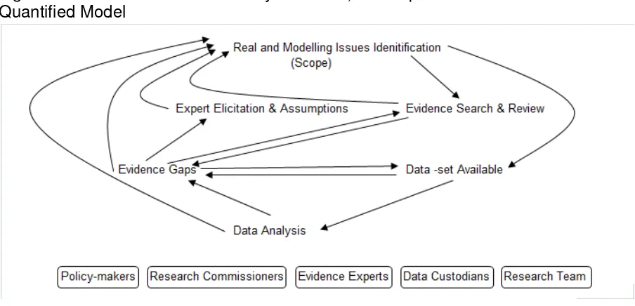
The central aim of our alcohol policy modelling framework is to estimate how the implementation of a policy will change, over time, outcomes of interest to policymakers and stakeholders. To do this, we need to be able to elicit relevant policies and outcomes, represent the relationship between policy (and potentially other environmental factors) and outcome, and to construct a baseline from which effects can be projected. In developing the Sheffield Alcohol Policy Model framework, a series of interlinked and iterative processes were undertaken (
[image:5.595.73.525.242.460.2]Figure
1
).Figure 1: Iterative Process to Identify Evidence, Develop Evaluation Framework and
Quantified Model
Throughout the process an interactive engagement continued between policy-makers, research commissioners, experts on the various domains of evidence, custodians of datasets which emerged as useful, and the research team itself.
At the centre of the process was the interaction between identified issues and the systematic search for and review of published evidence. For example, the Department of Health research questions specified three systematic reviews to be undertaken (Booth et al., 2008). They covered (a) the relationship from alcohol price to consumption or directly to alcohol-attributable harm, (b) the relationship between advertising/promotion to alcohol consumption or harm, and (c) a review of reviews on the relationship between alcohol consumption and alcohol-attributable harms (appropriate because there already existed considerable research and a number of recent reviews in the area). The resulting 243 page report was a key resource in developing the modelling framework e.g. identifying two recent meta-analyses of international price elasticities by Gallet (Gallet, 2007) and by Wagenaar (Wagenaar et al., 2009), which provided information on both possible methods and potential model parameter estimates. A similar approach of targeted systematic reviews agreed with policymakers/research commissioners was undertaken for the NICE project (Jackson et al.,
2009a;Jackson et al., 2009b).
available on the key components of the system, and early analyses of these data sets enabled the modelling team to evaluate what would be possible in terms of integrating the published evidence and the UK available data. Policy-makers and research commissioners were also involved in this
process, particularly regarding where special data analysis exercises by government departments or the potential purchase of access to commercial datasets. As thinking developed, the analysis of evidence and data-sets fed back into identifying more detailed issues to address e.g. exact definitions of the different metrics for outcomes (e.g. defined sets of crimes), with this in turn followed by a further cycle of evidence and data review. In some cases evidence gaps remained after iterative searching. These factors cannot be ignored just because the evidence base is limited, and a process of
considering assumptions by the research analyst or by eliciting information from experts was undertaken.
Decisions concerning whether to go into further detail in the modelling, when to elicit further expert opinion, or undertake specific sensitivity analyses were made by balancing principled and pragmatic
considerations: on the one hand ‘shouldparticular issues or details be included in principle?’, and on the other, ‘what is the likelihood of additional work affecting model results substantively?’. Here, it was fundamentally important to have clear research questions for the model to answer - one cannot prioritise further modelling effort without having at least an implicit metric for assessing the difference further detailed modelling would make to decisions.
Policy-makers and research commissioners were particularly important in iterative discussions on three aspects of the research scope. The first concerned the definitions of population subgroups for which separate results would be necessary. More details are given later, but one example was the decision, some way into the Department of Health project, to incorporate ‘moderate drinkers’ within the model, thus enabling a whole population analysis not just a focus on the four original subgroups, and the related decision to drop a separate focus on low income groups as it became clear that differential evidence for this subgroup was limited, and that the resources required to model both low income and moderate drinkers separately were beyond the project budget. The second aspect of scope concerned refined definitions of the exact policies to be tested, as both early results and understanding of the potential for implementation developed. The third concerned which dimensions of effect were most important to quantify and how each should be valued. A partial cost-benefit analysis approach has been taken, with monetary valuation of population health effects (QALYs), NHS direct costs, monetary valuation of crime victim QALY effects, criminal justice system costs, work absence and unemployment effects valued at average salary rates. Again, more detail is given later, but key decisions limiting scope of effects included: analysing alcohol industry changes only in terms of retailer income and not subsequent knock-on effects through the supply chain, analysing wider economy effects only in terms of work absence and unemployment, and excluding analysis of drinker benefits/utility/consumer surplus.
A set of what we now consider generic components for the evaluation of public health strategies emerged from these processes. In the next sections we go through each component in turn describing how it has been addressed in Sheffield Alcohol Policy Model framework.
Classification and definition of population subgroups of interest
Three influences led to our final subgroup definitions. The first was the research brief, which implied
the need to define age groups, ‘binging’ and ‘harmful’ drinking because of a request to focus on
underage drinkers, 18-24 year old binge drinkers and harmful drinkers. The second was the
availability of data on levels of consumption and purchasing of alcohol. Here, two key sources of data emerged from our searches. The General Household Survey (GHS) collects cross-sectional
during any one day during the past week (peak day consumption) (Office for National Statistics: Social and Vital Statistics Division, 2008). Consumption estimates are split by type of alcohol. The GHS contains no information on prices paid or purchasing patterns. The Expenditure and Food Survey (EFS) is another annual cross-sectional household survey (different individuals from those in GHS) using a 14 day diary to record household purchases including all alcohol items purchased, the type of alcohol, the place of purchase (on-licensed vs off-licensed sector) and crucially the price paid per volume of product (Office for National Statistics and Department for Environment Food and Rural Affairs, 2008). The third influence was indirectly due the types of harms to be examined and the metrics for their valuation. The UK government had previously examined harms attributable to alcohol in terms of health e.g. lives lost, as well as crimes committed and costs to employers (Health Improvement Analytical Team, 2008). Since the years of life lost if someone dies as a consequence of their alcohol consumption are related to their age, and since employment costs are related to workforce participation, we felt it necessary to extend the age-sex groupings to a broader set than those implied by the original research funder questions.
Eighteen age-sex subgroups were defined as males/females with age bands 11-15, 16-17, 18-24, 25-34, 35-44, 45-54, 55-64, 65-74, and 75+. Each age-sex group is further split into 3 drinking level
groups defined as: moderate drinkers with an alcohol intake within the UK government’s
recommended limits, defined as 168g/week or less for men and 112g/week or less for women; hazardous drinkers, defined as exceeding those limits but drinking less than 400g/week for men and 280g/week for women; and harmful drinkers with a weekly intake of more than 400g/week or
280g/week for men and women, respectively. (The UK defines a ‘unit’ of alcohol as 10 millilitres, approximately 8g, of ethanol). This resulted in 54 defined subgroups to be modelled. Individuals in
the GHS sample were also classified as a ‘binge drinker’ or otherwise based on the maximum intake of alcohol during one day of more than twice the recommended daily limit i.e. more than 64 g/day for men and more than 48 g/day for women.
Identification and Definition of Harms and Outcomes for Inclusion
For health harms, our literature review quickly identified recent UK work on the health harms attributable to alcohol (Jones et al., 2008). This used routine data sources to estimate, for each person in the population according to their age group and gender, the risk of mortality and
hospitalisation related to 47 different alcohol-attributable health conditions. Conditions were classified as wholly attributable to alcohol (no cases would exist in the absence of alcohol consumption, for example alcoholic liver disease) or partially attributable to alcohol (a proportion of cases would be avoided in the absence of alcohol, e.g. throat cancer). Conditions were also classified as chronic or acute, depending on whether the condition typically arises through long-term overconsumption (e.g. liver cirrhosis) or can arise through overconsumption on a single occasion (e.g. falls or road traffic accidents).. Modelling of both mortality and hospitalisation rates later enabled assessment of Quality Adjusted Life Year (QALY) effects and hospital costs. Further systematic review on health harms found few conditions to add, and we decided to build the modelling of health harms to the individual on this detailed foundation. Wider harms were discussed in the literature, but were less well
evidenced with little quantitative data (e.g. ‘passive’ heavy drinking effects on partners and children)
and were excluded due to limited resources for primary research within our project.
analyses). To apportion crimes into our population subgroups, we used separate routine data on the distribution of offenders found guilty or cautioned in 2003 (ONS, 2005) for the age groups 10-15, 16-24, 25-34, 35+ for 7 offence categories, making assumptions about the mapping between these 7 offence categories and our 20 crime classifications, splitting the 16-17 from the 18-24 year olds (assuming equal probabilities) and disentangling the 10 year bands for those 35+ (assuming linearly decreasing crime rates with age).
For workplace harms, the government had examined work absence, unemployment and lost outputs due to early death (Health Improvement Analytical Team, 2008). We excluded the latter to avoid double counting the social value of life years lost which we already modelled in health and crime harms. For absence, we initially planned to use the ‘Whitehall 2’ civil servants study (Cabinet Office/Strategy Unit, 2003) containing data on alcohol consumption also absence from work ‘due to
injury’ or ‘for all reasons’. However this had an endogeneity problem. On the one hand, people who drink heavily might be more absent from work (causal), but on the other hand, those absent with significant illness may be less likely to drink alcohol (unrelated) – and this latter appears to be the dominant factor in that dataset. Instead we used an Australian study (Roche et al., 2008) which explicitly asked respondents whether their absence was caused by alcohol, to quantify a relationship between reported absence days caused by alcohol and level of alcohol consumption itself. For unemployment we used the same evidence as the previous government reports (Cabinet
Office/Strategy Unit, 2003), i.e. a study (MacDonald et al., 2004) which examined Health Survey for
England data for males aged 22 to 64 and found that being a ‘problem drinker’ (defined using
psychological/physical symptoms or quantity/frequency of consumption), reduced the probability of being in work by 6.9%. We assumed the same figure for females but adjusted taking account of differential work participation rates by age-sex group.
Classification of modifiable components of risk and their baseline values
The key modifiable risk factor is level of alcohol consumption for individuals and, following a review of available datasets measuring consumption, we utilised the General Household Survey (GHS 2006) to provide the baseline. For each sample individual, weighted at the household level to be representative of a proportion of the population, we accessed details on mean weekly consumption of standard alcohol units (enabling grouping into moderate, hazardous and harmful), and maximum per day intake in the survey week enabling a proxy analysis of binge behaviours (14,289 individuals excluding outliers). We split consumption into 4 beverage categories because prices might change differentially under different policies: beers, wines, spirits and ‘Ready-To Drinks’ (RTDs or ‘alcopops’). Data for those aged 11-15 came from the school-based Smoking Drinking and Drug Use (SDD) Survey (REF) which used the same consumption definitions as GHS and assumed individuals had equal sample weight.
Specification of baseline position on policy variables (prices, availability, advertising)
sources including the ONS (Goddard, 2007). We analysed anonymised individual EFS diary data, at
purchased item ‘transaction’ level, (obtained via request to the government Department for
Environment, Food and Rural Affairs), for 69,618 individuals, of whom 44,150 purchased alcohol over 5 years 2001/2 to 2005/6, accounting for inflation using RPI inflators for alcoholic beverages. We found discrepancies between the distribution of purchase prices from the EFS and higher level data, which we obtained from market research companies on alcohol sales of beers, wines, spirits and alcopops in the off-trade (AC Nielsen) and on-trade (CGA Strategy). EFS reported data had
marginally lower mean prices (i.e. a higher proportion of cheaper alcohol) than the actual sales data. We therefore used linear interpolation to adjust the individual level EFS data so that the adjusted cumulative price distribution matched the actual sales data price distribution at 10 specified price points. With this data, we were therefore able to examine in detail the types and prices of beverages purchased by each of the 54 different population subgroups (for detailed examples see Table 1 in (Purshouse et al., 2010b)).
To analyse the existing extent of price promotion discounting, we obtained further analyses of market research data for both the off-trade and on-trade via procurement from AC Nielsen and CGA Strategy respectively. The underpinning data was at stock-keeping unit (SKU) level e.g. a specified branded pack of 4*300ml bottled beer. Price information is held weekly and, using a conventional definition of discounting as a less than four week price reduction for a SKU, our suppliers were able to analyse the
‘usual price’ and the ‘sold price’ and construct aggregated summaries of discounting. This was done in 10 defined price per unit of alcohol bands enabling estimates, for example, of the volume of off-trade beer with a usual price of 35-40p per unit which is actually sold at 30-35p, 25-30p etc. We were then able to use these patterns of discounting to estimate the effect of policies that restricted
discounting to a certain level (e.g. a total ban on off-trade discounting, or banning buy-one-get-one free but allowing five-for-the-price-of-four, etc).
For availability and advertising analyses, we found an evidence/data gap regarding publically available national level data on outlet densities, opening hours and volume of advertising/marketing effort. It was not possible to establish a robust baseline for England for any of these factors, or their relationship to current patterns of consumption in England. In the next section we discuss how a high level relative change approach has been used to give policy-makers some guidance on the potential scale of effects.
Estimating Effects of Changing Policy Variables on Risk factors
In order to estimate the effect of a pricing policy on an individual’s alcohol consumption the model
used an econometrics model which was derived using the adjusted EFS dataset. The econometrics model is a system of simultaneous equations relating consumption to price for the 16 modelled beverage types and also the consumption of other non-durable goods. Covariates were included for gender, age group, ethnicity, education, geographical region, household composition, household size, income and employment status. The coefficients for this system of simultaneous equations were estimated using an iterative three-stage least squares regression. Due to the volume of data
It was not possible to apply this approach in order to estimate peak consumption price elasticity due to the absence of adequate data relating peak consumption to purchasing. The alternative approach that we adopted is based on the observation that in the GHS the probability and scale of peak/binge drinking is related to the mean weekly consumption. Separate linear models were estimated for each drinker type (moderate, hazardous and harmful) while the coefficient of mean consumption was allowed to vary for each gender and age group.
For advertising policies, including the use of positive public health messages, eliminating exposure of
under 18’s to advertising and a total ban, only a small number of studies provide elasticity estimates relating advertising expenditure to changes in alcohol consumption. Elasticities were selected from the literature (see detail in (Purshouse et al., 2009a) report to NICE) and the resulting relative change in consumption is applied to all simulated individuals affected.
For availability policies, including changes to the density of outlets and restrictions in hours of sale, again, elasticities were selected from the limited literature (see detail in (Purshouse et al., 2009a) report to NICE) and the resulting relative change in consumption applied to all simulated individuals affected. The availability analyses were of a high level ‘what-if’ kind (e.g. what if outlet density were reduced by 10%) because detailed policies relating to outlet licensing are implemented at a local level often in tandem with other interventions such as server training, whilst national level policies are usually legislation based and act as an enabler for local action,
Risk Functions Relating Risk Factors to Harm
An epidemiological approach was used to model the relationship between consumption and harm, relating changes in the prevalence of alcohol consumption to changes in prevalence of harmful outcomes. Five inter-related concepts are involved:- the total absolute level of harm occurring in the population, the alcohol attributable fraction, absolute risk functions relating the risk of harm to the level of alcohol consumption, relative risk functions relating the relative risk (RR) of harm to the level of alcohol consumption, and the potential impact fraction which calculates the change in harms following a change in consumption levels.
We categorised health harms for 47 ICD diagnosis defined conditions into 4 types: chronic harms related to mean alcohol consumption and acute harms related to peak day consumption, with a further split into conditions wholly or partially attributable to alcohol.
For chronic illnesses that are partially attributable to alcohol (e.g. oesophageal cancer), we were able to take evidence directly from published literature which provided continuous risk function curves relating mean weekly alcohol consumption in units to an individual’s relative risk (RR) of mortality or disease prevalence differentiating by sex when available (Corrao et al., 2004;Gutjahr et al.,
2001;Hamajima et al., 2002;Rehm et al., 2004). We assumed that the relative risk curves are the same for each age group but that absolute risk levels differ for each age/sex group. We have direct published data on these mean absolute risks for each age sex group at baseline (e.g. annual mortality rate for oesophageal cancer for males aged 45-54) and therefore we have enough information to compute the change in absolute risk for the subgroup when the distribution of consumption changes following a policy. This change in absolute risk is calculated by multiplying the baseline absolute risk
by the potential impact fraction (PIF) (Gunningschepers, 1989). 0
0
1
N i i i N i i iw RR
PIF
w RR
where wi is the sample weight for observation i (e.g. an individual sample from the GHS) and N is the
that individual’s baseline consumption level, and and is the modified risk for individual i given their new consumption level following the policy change.
For the other three types of harm, published continuous risk function curves were not available and we developed a method to derive our own continuous risk function curves from the broader data that were available. Under this method we developed two-part linear risk functions whereby the risk is flat from zero consumption up to a particular threshold and then rises linearly as consumption increases. For each harm and age/sex subgroup it was therefore necessary to decide on an appropriate threshold after which the risk function begins to rise, and then to estimate the slope of the rising straight line risk function beyond that threshold to fit the available observed data. The central idea is that we know the distribution of alcohol consumption in England (from the GHS), we have or can derive estimates of alcohol attributable fraction (AAF), and therefore it is possible to fit a linear risk function that implies the same AAF as that observed. For acute health harms that are partially attributable to alcohol (e.g. fatal road traffic accidents), published evidence did exist on the alcohol attributable fraction (AAF) (e.g. 37% of fatal road traffic accidents for men aged 25–34 are attributable to alcohol) (Jones et al., 2008). We assumed RR is a function of peak daily consumption, with RR=1 below a threshold of 3 units for women and 4 for men, and then estimated the slope of the risk function beyond the threshold by fitting the slope using ordinary least-squares regression to minimise the difference between the implied predicted AAF (the implied risk for those GHS samples with consumption above zero divided by the implied risk for the whole subgroup) and actual observed AAF for the age/sex subgroup.
For health harms wholly attributable to alcohol, a very similar approach was taken. For acute health harms which are wholly attributable to alcohol the AAF=1 by definition, and we used a similar two part linear risk function approach instead using the total observed volume of incidents (e.g. annual mortality rate for accidental poisoning by exposure to alcohol) as the metric to fit the slope of absolute risk functions in each age/sex subgroup. For chronic diseases wholly attributable to alcohol, we used the same two-part linear approach except that the risk function is related to mean weekly consumption with an assumed threshold for the start of rising risk of 2 units per day for women and 3 for men. Having estimated our own continuous risk functions for each of these types of harm, the change in risk implied by a consumption change following a policy can be calculated using the PIF.
Finally, for the chronic illnesses, debate exists about the time lag between change in exposure and change in risk (Norstrom et al., 2001). We chose a linear lag function of 10 years to realisation of full effect i.e. the full estimated reduction in risk only occurs after 10 years and in the years between the risk reduction is linear so that at year 1 it is 1/10th of full effect, at year 2 it is 2/10ths etc. The 10 year assumption is consistent with average estimates from the literature and was varied this in sensitivity analyses.
Crime was assumed to be partially attributable to peak alcohol consumption and we used the same approach to fit two-part linear RR functions as for partially attributable acute health harms. The AAF for every category of crime was derived from the Offending Crime and Justice Survey (OCJS) for England and Wales in 2005, using the questions which ask convicted offenders whether they had undertaken the offence because they were drunk (Home Office.Research, 2011). RR functions were estimated for males and females and for two age groups, under 16 and between 16 and 25,
separately from the OCJS. The same RR functions were used for over 25’s based on those for 16-25,
which is a limitation, but may not greatly impact on the modelling results as over 25 years old contribute to less than 30% of all alcohol attributable crimes. Again, the change in absolute risk following change in consumption is calculated using the PIF.
between changes in prevalence of consumption and the changes in the risk of not working. We used the same two-part linear approach to fit unemployment RR functions, using a mean consumption threshold of 5 units per day for women and 7.1 for men (i.e., thresholds defining harmful drinkers). The AAF for unemployment was estimated based on the assumption of reduced probability of working
for “problem drinkers” of 6.9% (MacDonald et al., 2004) which was also used by the Cabinet Office in the UK to estimate the impact of alcohol misuse on unemployment (Cabinet Office/Strategy Unit, 2003). We then used the change in mean consumption to adjust observed absolute unemployment figures (from the Labour Force Survey 2006) using the PIF.
Absenteeism was assumed to be partially attributable to alcohol and relate to peak alcohol consumption, again using the two-part linear approach to fit RR functions for each age/sex group. The AAFs for absenteeism were derived from the Australian study (Roche et al., 2008); the only one identified which examined the causal relationship between alcohol and absence from work. The change in peak consumption then adjusted the baseline number of absent days for each age/sex subgroup (from the Labour Force Survey 2006) using the PIF.
?
Monetary Valuation
The first dimension of monetary valuation of the effects of policies is the direct financial effects of
policies on consumers’ spending, retailer and government revenues when alcohol purchasing
patterns change. Using the EFS purchasing data the model is able to estimate an overall change in the volume of sales (in units of alcohol) for beers/wines/spirits/RTDs to each age/sex/drinking level subgroup and the associated value of sales (in £s). When modelling price rises the level of consumer spending typically increases, and we model the overall change in retailer income separately for on-trade and off-on-trade but not by different particular named or types of retailer. To assess changes to government revenues, the sales value for each beverage type is apportioned into money to the retailer, alcohol duty to government and value-added tax (VAT). The average rate of duty per unit of alcohol for each beverage type was derived from work conducted by the Department of Health [Ref 1], VAT was assumed to be 17.5%. The knock-on effects within the alcohol supply chain to manufacturers, transport companies, growers etc. is not modelled.
The second dimension of monetary valuation concerns the health, crime and workplace harms. The annual cost health harms includes the direct cost incurred by the NHS, through providing treatment or services, and also the monetary valuation of the change in population quality of life using a value for a quality adjusted life year (QALY). A Department of Health report (Health Improvement Analytical Team, 2008) provided the annual NHS cost of treating most diseases attributable to alcohol, with most conditions broken down by type of consultation/service though we had to apportion some costs using the expert opinion of clinical colleagues. For diseases not covered by this report, we derived cost estimates using the average tariff from the NHS reference costs and the number of hospital admissions from Hospital Episode Statistics using the NWPHO report (Jones et al., 2008). Health related quality of life measures for each condition were extracted from the Health Outcomes Repository database (Health Outcomes Data Repository, 2011) which measures QALYs using the EQ-5D around 6 weeks after hospital discharge. Following direction from the Department of Health, a quality adjusted life year was valued at £50,000 and discounted at the standard rate of 3.5%, while health care costs were discounted at 1.5%.
The valuation of workplace harms, which includes absence due to sickness and unemployment, were quantified based on average earnings in each age/sex group. Although costs to the public sector could also include unemployment benefit payments, these were not included due to debate as to whether these resources are lost or are in fact redistributed (Office for National Statistics, 2011).
Model Structure to Integrate Harms Analysis (Modelling event histories)
The model is a hybrid model mostly operating at the resolution of population sub-group level with 54 sub-groups defined by sex, age and baseline alcohol consumption level. The vast majority of the model parameters are defined at this level. However, parameters relating to the alcohol consumption distributions (both mean daily and maximum daily) and alcohol purchasing distributions (across 16 categories of beverage) have a much more detailed level of resolution, being defined in terms of the sample individuals from the GHS or sample transactions from the EFS respectively. These samples essentially describe empirical non-parametric distributions of consumption and purchasing.
Adjustments to both prices and consumption are made at the individual sample level, whilst effect sizes are calculated at an aggregate i.e. subgroup level.
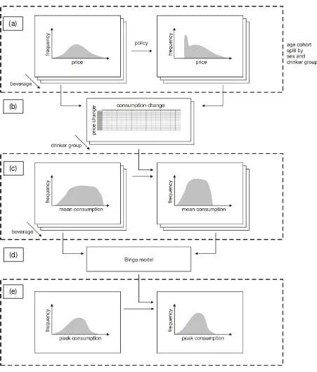
Figure 2: Policy-to-consumption model schematic
(a)
(b)
(c)
(d)
Figure 3 illustrates how these revised mean and peak consumption distributions for the subgroup are then used to calculate harm changes via the risk functions and PIF approach. Figure 3a illustrates that the modelling of harm is formulated as a comparison of two possible futures in terms of consumptions, Future A versus Future B. In most applications of the model Future B consumption has been left at current baseline levels. The modelling begins with the baseline consumption distributions and looks forward 10 years in terms of consumption distribution trends for age age/sex subgroup. By far the most difficult aspect of model structuring concerned how to deal with various aspects of time passing in a coherent way, including the cohort ageing each year, the fact that there can be lags in harm effects, and that differential proportions of each subgroup die each year when comparing Future A and Future B.
Figure 3b illustrates that the revised absolute annual risk of mortality for each of the 47 health conditions is calculated each year for each age/sex cohort. Because there is a lag structure for the chronic conditions, the consumption distribution in year 1 affects not only year 1 risks but also those in year 2, year 3 and up to year 10. Thus in year 1 in Future A, the change in risk is due to 1/10th of full effect of the consumption distribution change between baseline and year 1. In year 2 in Future A, the change in risk is due to 2/10ths of the full effect of consumption distribution change between baseline and year 1, and 1/10th of the full effect of the consumption distribution change between baseline and year 2. Thus the changes in consumption over the years accumulate over time in terms of computing revised absolute risks of mortality. Not shown but also calculated is the revised absolute risk of disease prevalence for each condition for each age/sex subgroup, as measured by the proxy indicator of person specific hospitalisations for the disease.
Figure 3c illustrates how these revised annual risks are then applied to each population age/sex group cohort over time to calculate the survival, QALY and cost effects of consumption changes over time. The age-cohort approach models people in a particular age band (e.g. males aged 45-54), ignores the issue that this age band will be made up of different constituent members at different time points and assumes that the population distribution of drinking is stable over time within the age band. As model time progresses one year at a time, a calculation is done to quantify the estimated
proportion of people in the subgroup who die within the model year from each condition. The difference between the numbers dying in Future A and Future B in the model year is calculated and the difference in QALYs lived is estimated by a life-table for the normal population adjusted for age/sex estimates of utilities for the average population. A second calculation is done to compute the prevalence of each of the conditions in the model yea, the QALY decrement due to being alive with the condition in the year and the associated in year treatment cost.
It is important to emphasise that the model is not a micro-simulation, operating on individuals within a cohort. The individual level data are merely used to describe non-parametric distributions for a sub-group. Effect sizes in most applications of the model to date are sub-group averages, assuming the entire sub-group has been impacted by the same percentage change in consumption. This
Figure 3: Consumption-to-harm modelling schematic
RESULTS
Results Framework
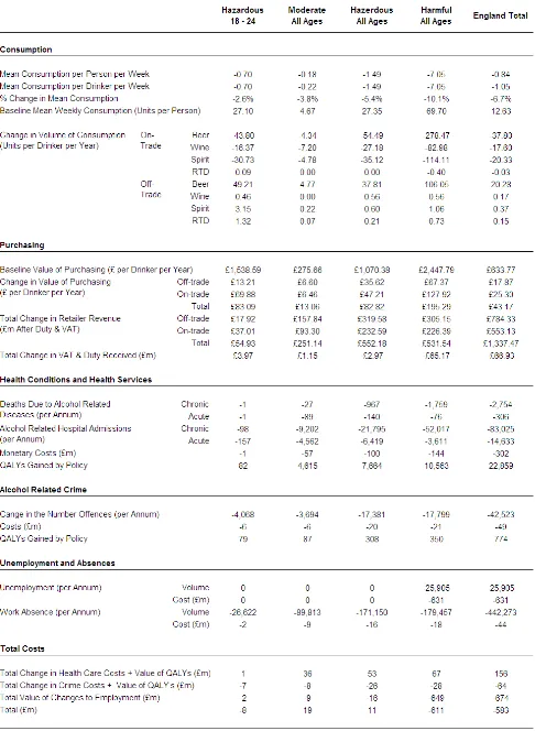
Model results can be presented in substantial detail for a single policy. Table 1 illustrates results for a 50p minimum price per unit policy for subgroups of hazardous drinkers aged 18 – 24, moderate, hazardous, and harmful drinkers of all ages, and the whole population. Results for consumption levels indicate baseline consumption, mean reduction in consumption, and a split by beverage type, so that policy-makers can see which subgroups and types of alcohol are most affected in both relative and absolute terms. Results for purchasing indicate the mean change in spending per year for different subgroups, both on-trade and off-trade, together with the effects on changes in government (VAT and duty) and retailer revenues. For health, crime and workplace harms the model results can show details on the volume of annual incidents e.g. reduction in violent crimes or reduction in deaths due to road accidents annually, and these can be summarised at broader levels such as
acute/chronic disease mortality and hospitalisation rates. Monetary costs to the health service and criminal justice system are shown. QALYs gained by the policy are shown, both health and crime related. Workplace harms and their monetary valuations are also shown, again allowing policy-makers to examine how these estimated effects compare between say moderate, hazardous and harmful drinkers. In moving towards a partial cost-benefit analysis approach, the monetary valuation of the harm reduction across health, crime and workplace harm is combined, allowing policy makers an indication of the relative effects across these three sectors and a summary total.
19
One way and multi-way sensitivity analyses have been undertaken (Purshouse et al., 2009a). Most were straight forward parameter estimate changes e.g. changing the time lag assumption for chronic health harms from a basecase 10 years to either 5 or 15 years to see the effects on results. The most complex of the sensitivity analyses have related to the structural form of the price elasticity estimates and the data used to derive them. Five examples are discussed here. First, basecase elasticity matrices were estimated for two groups, moderate drinkers, and hazardous and harmful drinkers combined, but other published evidence suggests there may significant differences between age/sex subgroups too. We undertook a sensitivity analysis attempting to account for this by weighting the cross-price elasticity estimates based on the difference between the preference vector of the particular subgroup and the preference vector for the aggregated groups. Second, for some age/sex subgroups the EFS purchasing data does not provide a good match when compared with the GHS consumption data, partly due to purchases by one person being consumed by another, so we reallocated purchases where this seemed plausible and obtained an improved match between the EFS and GHS consumption data. Third, the elasticity estimates derived using the econometrics model showed heavy drinkers as slightly more responsive to price change than moderate drinkers, and we carried out a sensitivity analysis to explore the changes to the model results if heavy drinkers are assumed to be one third less responsive than moderate drinkers (Chisholm et al., 2004). Fourth, we undertook a set of analysis using completely different, previously published long run UK elasticity estimates from Huang 2003 (Huang, 2003) based on high-level time series data, in which both own-price and cross-price elasticity estimates are greater than those derived from EFS. Finally, probabilistic sensitivity analysis was used to explore the impact of uncertainty in the coefficients of basecase elasticity estimates from the regression using Cholesky decomposition, with the resultssuggesting that the parameter uncertainty around these coefficients is much less significant that the structural assumptions described above.
20
DISCUSSIONScope and Monetary Valuation Issues
There are extended challenges in applying economic modelling to macro-level interventions, beyond those commonly encountered say in NICE health technology assessments. In particular, the range of costs and benefits to be included can be difficult to determine, especially when decision-maker and stakeholder concerns may not be limited to the immediate and direct effects of an intervention. Direct Policy implementation costs to government for regulation of alcohol prices, advertising, outlet density or licensing hours are likely to be minimal (consisting of legislative processes, implementation and enforcement through existing mechanisms) and as such we have to date excluded these from the detailed analysis. Valuation of health and crime harm reductions have been estimated using a quality adjusted life years gained framework (to patients and victims respectively), with a financial value for a health-related QALY and a crime-related QALY applied. Valuation of workplace harm reductions, i.e. sickness absence and unemployment, were quantified financially based on average salaries.
Some might argue for a purely public sector stance to be taken by decision-makers, whereby for example, larger price increases produce greater estimated harm reductions with relatively small public sector implementation costs i.e. ever larger price increases would be considered more
‘cost-effective’. From a public sector perspective some might argue that costs of the lost
productivity from public sector employees should be included and also possibly any government costs relating to sickness and unemployment benefit payments for the whole population. There is some debate about the latter costs, since it could be argued that these should be treated as transfer payments (a redistribution of income in the market system which does not directly absorb resources or create output) and therefore be excluded. At present we have examined workplace costs for the whole population, not separating public sector from non-public sector.
Costs to individuals (either drinkers themselves or to their family, friends and colleagues) were outwith the scope of the NICE economic assessment, although they may be considered in terms of equity implications. In the original analyses for DH, we analysed increased expenditure by consumers. Such direct effects were included at the request of policymakers. For retailers, the model produces estimates of changes in volumes of alcohol expected to be sold as a
consequence of each policy, which are then combined with price information to derive, for the country as a whole, the retail sales value (£) of different types of alcohol in both the off-trade and on-trade. These estimates are not broken down by type of retailer or particular named retailers. Nor do they make any estimates of profit or otherwise from alcohol for retailers since analysis of
retailers’ cost-base are not included in the modelling. Similarly, there is no quantified assessment here (beyond the retail sales overall) of the potential impact on different producers of alcohol, since direct information on their costs, the wholesale market, and the profit made by producers in selling on to retailers are not covered by the modelling.
Some other transitional costs are not examined here, including effects on the advertising or media industry. It is important not to misinterpret the increased costs to consumers and increased sales values to retailers: the changes in consumer expenditure under the different
21
workforce savings) should be balanced. This is because the increased expenditure by consumers has to be considered in conjunction with the increased revenue to the alcohol industry(producers, wholesalers and retailers) and possibly reduced revenue to other sectors of the economy. The increased revenue to the alcohol industry will return to the wider economy in a variety of ways; for example, wages and salaries to industry employees, profits to individual and institutional shareholders, including pension funds, and potential price reductions on other goods where retailers have been using alcohol as a loss leader. The analysis presented here does not include this dynamic analysis of the full effects of redistribution through the economic system.
Expected changes in tax revenue income to government were also modelled. Again these are
not ‘net effects’ and were included for information, rather than for direct trade-off calculations in relation to public sector benefits. If increased revenue were to accrue to the Treasury, then this also can be conceived of as returning to the wider economy in the form of increases in
government services or reductions in other taxes. The public sector focus of NICE economic evaluations also excluded consideration of welfare losses (typically defined by consumer surplus as an economic measure of consumer satisfaction based on the difference between the price of a product and the price a consumer is willing to pay) arising from reduced consumption of alcohol. Consumer welfare analysis has not been undertaken as part of this study. Such an analysis would need to account for potential increases in consumer surplus from any price reductions
elsewhere in the economy and the problems of estimating a ‘pure’ demand curve for alcoholic
beverages.
Limitations due to data and evidence gaps
Ideally, price analyses would be based on longitudinal data recording both alcohol consumption and purchase. Such data is not available in the UK and we chose to use the annual cross-sectional EFS purchasing data which provides information on alcohol volumes and prices paid at an individual level. However, it may not be appropriate to assume that the consumer is the purchaser (i.e. if alcohol purchased by one household member is then consumed by a different household member). The current econometric model, although it does allow some of the complexity of the problem to be modelled, remains a relatively simple approach, especially with zero purchase observations (people who did not buy alcohol during the 14 day diary period) not modelled separately from non-zero observations. A new longitudinal survey obtaining both price and consumption data would be very valuable in such a context.
Peak consumption was estimated from the GHS, in which respondents were asked how much they consumed on the heaviest drinking day in the past 7 days before the interview. We then used this as a proxy for binge drinking. Binge drinking would be better represented by a combination of both frequency of heavy drinking occasions and average consumption level on such occasions, if such data were available.
22
We assumed no delay between price-based policy implementation and price changes, effective enforcement/full compliance of supply-side with the policy and that only targeted products would be affected. For example, in our model a minimum price for spirits does not lead to price changes in products other than spirits. This assumption ignores market response to price changes.Research analysing the supply-side response to pricing policies is desirable, because it is plausible that policies that have a large effect on beverage prices might lead to market
restructuring, and supply-side responses are unlikely to be straightforward (Kenkel, 2005;Young et al., 2002).
We assumed a linear time lag between a change in consumption and a change in mortality and morbidity risk for all chronic illnesses, however, different illnesses may have different lag structures (e.g., liver cirrhosis vs breast cancer) and the change of risk may be the same each year. Further systematic review and analyses would help identify disease specific and more sophisticated time lag structure and improve the understanding of the relationship between changes in consumption and changes in risk, for different types of harms. We also assumed that a type of harm is either related to mean consumption or to peak consumption, however, some types of harm may be caused by a combination of mean and peak consumption (e.g., suicide, heart disease). There is also no consensus on the threshold above which risk begins to increase, especially for acute harms, the current model assumes 32g / 24g per day for acute harms and 24g / 16g per day for chronic harms, for male and females respectively. In general, risk modelling is better developed for health harms than for crime and workplace outcomes, especially
unemployment. Further research is needed to examine what proportion of these outcomes is attributable to alcohol.
Further developments
The current model is able to appraise a wide range of price-based policies including general price changes, minimum pricing and some policies affecting availability measures and advertising restrictions. However, the evidence on the effectiveness of price-based policies is more robust and abundant than for availability measures. Further research to examine the effectiveness of availability measures and potential policy mix (e.g., simultaneously introducing availability and price-based policies) would be useful.
We used 2006 data for alcohol consumption and purchasing as the baseline and did not consider underlying trends, thus implicitly assuming steady-state alcohol consumption in the “do-nothing
scenario”. It is challenging to validate the current model against historical data because of other
factors affecting alcohol consumption, such as changes in disposable income and licensing hours, arise simultaneous to price changes. Further analyses to identify the underlying trends in
alcohol consumption and further development of the model to establish a dynamic “do-nothing
scenario” will enhance the credibility of the model and facilitate model validation.
23
policy to consumption and from consumption to harms; 4) the development of new econometric models to address the limitations of the current method; 5) systematic review of policy context and its impact on policy effectiveness; 6) enabling appraisal of availability policies and policy mix; 7) development of a new dynamic model, which not only incorporate the findings of the rest of the project work packages, but also accounts for trends in alcohol price, income, consumption and harm.Adaptability of the Framework to Other Questions
Since the original framework was developed we have engaged in adaptations which have updated the analysis and results as new survey data has become available. Within England, the framework can be fairly easily applied to any intervention where there is an effect on alcohol consumption levels, for example, we have been able to adapt the model to produce estimates of the cost-effectiveness of screening and brief interventions for alcohol in a variety of different settings (Purshouse et al., 2009b).
Country adaptations of the model have also been undertaken and further adaptations are ongoing. Adapting to Scotland (Petra Meier et al.,) required use of different but very similarly structured datasets on baseline consumption, mortality, hospitalisations and crime. We are beginning the process of adapting the minimum pricing modelling to a province in Canada, and the screening and brief intervention modelling to Netherlands, Italy and Poland, all of which seem at this stage to be feasible, with the key issue being the adaptations required to incorporate each
country’s existing datasets around consumption, mortality, hospitalisations, crime and
employment.
In the UK, this work has been critical to a series of policy debates since the initial report for the Department of Health was written. In England, a weak form of minimum pricing has now been introduced, stipulating that no product can be sold below the cost of alcohol duty plus VAT.
There has also been a ban on some ‘irresponsible’ discounting practices in the on-trade sector. A key discourse, driven by industry stakeholders and parts of the media, has been around whether
price policies penalise low income drinkers (“punishment of the poor”). Other research groups
have sought to provide counterevidence (Record and Day REF, Ludbrook REF). Version 3 of the model will also include explicit modelling of the effects on different income groups. In Scotland, an initial attempt to introduce a 45p minimum unit price was narrowly defeated in parliament, when introduced by a minority government. Policies restricting price discounts were however approved. In the most recent election in Scotland, the governing party now has an overall majority and a minimum price is back on the political agenda. The key challenge for such a policy
remains the demonstration of ‘proportionality’ of the pricing policies as defined under EU law, i.e.
that the degree of interference in the common market is necessary to avoid significant harm. Detailed health economic models such as ours are ideally placed to provide relevant evidence on which such decisions can be based.
Conclusion