On an asymptotic method for computing the modified energy for symplectic methods

for symplectic methods

.

White Rose Research Online URL for this paper:

http://eprints.whiterose.ac.uk/83359/

Version: Accepted Version

Article:

Niesen, J and Moan, PC (2014) On an asymptotic method for computing the modified

energy for symplectic methods. Discrete and Continuous Dynamical Systems - Series A,

34 (3). 1105 - 1120. ISSN 1078-0947

https://doi.org/10.3934/dcds.2014.34.1105

[email protected] https://eprints.whiterose.ac.uk/

Reuse

Unless indicated otherwise, fulltext items are protected by copyright with all rights reserved. The copyright exception in section 29 of the Copyright, Designs and Patents Act 1988 allows the making of a single copy solely for the purpose of non-commercial research or private study within the limits of fair dealing. The publisher or other rights-holder may allow further reproduction and re-use of this version - refer to the White Rose Research Online record for this item. Where records identify the publisher as the copyright holder, users can verify any specific terms of use on the publisher’s website.

Takedown

If you consider content in White Rose Research Online to be in breach of UK law, please notify us by

VolumeX_{, Number}0X_{, XX}200X _pp.X–XX

ON AN ASYMPTOTIC METHOD FOR COMPUTING THE MODIFIED ENERGY FOR SYMPLECTIC METHODS

Per Christian Moan

Centre of Mathematics for Applications University of Oslo

Norway

Jitse Niesen

School of Mathematics University of Leeds

United Kingdom

Abstract. _{We revisit an algorithm by Skeel} et al. _{[5, 16] for computing}

the modified, or shadow, energy associated with symplectic discretizations of Hamiltonian systems. We amend the algorithm to use Richardson extrapola-tion in order to obtain arbitrarily high order of accuracy. Error estimates show that the new method captures the exponentially small drift associated with such discretizations. Several numerical examples illustrate the theory.

1. Introduction. Numerical simulation of conservative differential equations re-quires special care in order to avoid introducing non-conservative, or non-physical truncation error effects. For Hamiltonian ODEs or Euler–Lagrange equations orig-inating from variational principles there exists much evidence [6,9,11,14] that the proper discretization scheme should besymplectic [7, 9, 11,18]. In the Hamilton-ian case this can be achieved by imposing special conditions on classical methods or by methods based on generating functions [7]. In the variational formulation symplecticity is achieved by discretizing the action integral and carrying out a dis-crete variation [10]. In some cases these formulations and methods turn out to be equivalent by the Legendre transformation [8,10].

Focusing on the Hamiltonian side, symplecticity implies that the trajectory produced by the numerical algorithm is the exact solution [12] of another, non-autonomous “modified” Hamiltonian system close to the original one. Various sta-bility results for Hamiltonian ODEs then apply, leading to an understanding of the dynamics of such discretizations schemes [6, 9, 11, 15]. Early results on modified equations focused on the autonomous part [2,4,6, 13,14] and established that its flow is exponentially close to the numerical trajectory. This work was motivated by the bounded error in energy observed in simulations with symplectic schemes. The early results are contained in the newer results since the time-dependent part is exponentially small due to analyticity. Despite its smallness the non-autonomous term excites instabilities through resonances, one consequence being a drift in the modified energy. In simulations requiring millions of steps such as in molecular

2010Mathematics Subject Classification. Primary: 65P10; Secondary: 37J40, 37M15.

Key words and phrases. modified energy, symplectic integration, Hamiltonian systems, Richardson extrapolation.

dynamics [9,17] and celestial mechanics [19] these effects become significant and it becomes important to understand and control them.

Constructing the modified Hamiltonian is equivalent to evaluating many terms in the Baker–Campbell–Hausdorff formula, or its continuous analogue [13], a com-binatorially complicated task possible only for small systems and to a low order of accuracy. Recently, Skeel and coworkers [5, 16] devised a method for numerically computing the value of the modified Hamiltonian along the numerical trajectory, thus allowing us to track the possible drift in the modified energy. In this paper we modify their method to make it easier to implement and obtain high order, possibly at the cost of extra storage. The new method is based on the same idea, but it does not give identical results. We also provide exponentially small error bounds when the new method is applied in the asymptotic regime. It is then used to verify, and justify the theory of modified equation on several test equations and methods.

2. Modified equations. As alluded to in the introduction, the numerical solution of an ODE y′ = f(y) is interpolated by the exact solution of a modified ODE y′ _{=f(y, t). The modified equation is non-autonomous, but the non-autonomous}

part is exponentially small in the step size. More precisely, given an analytic vector fieldf and a one-step method defined by an analytic mapping Ψh,f, there exists an analytic vector field f(y, t), h-periodic and analytic in t, whose exact flow exactly interpolates the numerical trajectory {xn}, xn+1 = Ψh,f(xn). The construction in [12] starts by constructing a modified vector field ˜f(y, t) which is only C∞ _in t whose flow interpolates {xn}. This vector field is then transformed by a time-dependent coordinate transformation into a vector fieldf analytic int.

The domain of analyticity of ˜f plays an important role in the analysis, and we have found it useful to assume that ˜f is analytic for ally in a domain of the form

Dy:=

[

t>0

{z∈Cd_{:|y˜(t)−z|∞<r˜y}=} [

t>0

{z∈Cd_{:|ℑ(˜y(t)−z)|∞<˜ry}}

for some ˜ry > 0, where ˜y(t) = φt,f˜(y0) is the trajectory of the smooth modified

vector field ˜f. This domain is typically smaller than the domain of analyticity off, and depends on the numerical method. In the following we will use the sup-norm

kfkD= supz∈Dy|f(z)|∞. With these definitions the main result of [12] in the limit h→0 can be formulated as

Theorem 1. Let Ψh,f be a one-step method applied to the analytic vector field f,

and yn+1 = Ψh,f(yn) be the approximations obtained by iterating Ψ. Then there

exists a modified vector fieldf(y, t) =f(y) +r1(y) +r2(y, t)which ish-periodic int and analytic in(y, t)∈ D′ such that its exact flow satisfiesy(nh) = Φ_nh,f(y0) =xn.

In the limith→0 we have the estimates

kfk_D′ ≤ 2

1−ηkfkD

kr2k_D′ =O

kfkD h exp

−η 2πδ

kfkDeh

for0< η <1,0< δ <r˜y. The domain of analyticity of the modified vector field is

D′=

(z, τ)∈Cd_×C_{:|ℑ(z−y(t))|∞<r˜y−δ,|ℑ(τ−t)|<} ηδ

kfkDe

,

For a Hamiltonian vector fieldf and a symplectic numerical method [6, 7, 14], the modified vector field f is also Hamiltonian [4, 7, 9], with Hamiltonian H = H(y) +G1(y) +G2(y, t) where H, G1 andG2 are the Hamiltonians corresponding

to the vector fields f, r1 and r2, respectively. The change in the modified energy

along the numerical trajectory therefore satisfies d

dtH ={H, H}+ ∂ ∂tH=

∂ ∂tG2, where{F, G}:=Pm

j=1FqjGpj−FpjGqj is the Poisson bracket. By Theorem 1this drift is very small for smallh, thus motivating symplectic methods.

3. The method of Skeel et al. _{for computing the modified energy. Skeel}

and coworkers [5, 16] found an ingenious way of evaluating the modified energyH at the points {xn} for discretizations based on splittings [3]. Suppose we have an Hamiltonian given byH = 1₂pT_M−1_{p+U(q). An explicit splitting algorithm with}

step sizehis given by

forn= 0,1,2, ... ˆ

p0=pn, qˆ0=qn fors= 1 :S

ˆ

ps= ˆps−1−hasUq(ˆqs−1)

ˆ

qs= ˆqs−1+hbsM−1pˆs end

pn+1= ˆpS, qn+1= ˆqS end

(1)

leading to approximationspn+1= ˆpS,qn+1= ˆqS when ˆq0=qn, ˆp0=pnattn =nh. By choosing the coefficientsas,bsappropriately, a method of arbitrary high order can be found. The modified Hamiltonian can be found by representing the inner loop of (1) as a concatenation of exponential operators [7]

Ψh,f(p, q) = exp(−ha1Uq∂p)(p, q) exp(hb1M−1p∂q)· · ·

exp(−haSUq∂p) exp(hbSM−1p∂q),

whereby the Baker–Campbell–Hausdorff (BCH) formula is used to find an expres-sion so that Ψh,f(x)≃exp(hf ∂)(x).

The approach of Skeel et al. _{for computing values of the modified energy is to}

append one scalar equation to the numerical integrator, forn= 0,1,2, . . .

ˆ

p0=pn, qˆ0=qn, βˆ0=βn fors= 1 :S

ˆ

ps= ˆps−1−hasUq(ˆqs−1)

ˆ

βs= ˆβs−1−has(ˆqsT−1Uq(ˆqs−1) + 2U(ˆqs−1))

ˆ

qs= ˆqs−1+hbsM−1pˆs end

pn+1= ˆpS, qn+1= ˆqS, βn+1= ˆβS end

where β0 = 0. To understand how the modified energy can be recovered from {pn, qn, βn}, note that by Theorem 1 the numerical trajectory (pn, qn) is exactly interpolated by the flow of a Hamiltonian H. The discretization (2) is the dis-cretization of Hα = α2H(α−1p, α−1q) where β is conjugate to α, the so-called

homogeneous extension of H(p, q). The discovery in [16] rests on the fact that homogeneous extension is a Lie algebra homeomorphism. Thus, since H is con-structed by Poisson brackets as in the BCH formula, the modified Hamiltonian for (2),Hα, is the homogeneous extension ofH, hence the trajectory generated by (2) is interpolated by

q′=Hp(p, q, t),

p′=−Hq(p, q, t),

β′=qTHq(p, q, t) +pTHp(p, q, t)−2H(p, q, t),

from which

H = 1 2(q

T_H

q+pTHp−β′) =

1 2(−q

T_p′_+pT_q′_−β′_{). (3)}

The equation forαis removed from (3) sinceHαdoes not depend onβ, the conju-gate variable ofα, and henceα′_{= 0 which is solved exactly by the methods we are}

considering.

Thus the value ofH can be computed by finding the derivatives of the interpo-lating trajectory (which are not known since we do not have Hp, Hq). In [5, 16] estimates of the derivatives are computed using backward difference formulas and interpolating polynomials with stored values of {pn, qn, βn}. These polynomials can be precomputed, but unfortunately the required expressions are very large, and they only provide expressions up to order 24. Their method does however have an advantage in requiring less stored values than one based on centered differences, which might be important if the modified energy is part of the simulation [5].

4. Richardson extrapolation. Our suggestion is to use Richardson extrapolation in order to avoid the large expressions that arise in the method described in the previous section.

First consider the use of Richardson extrapolation to find the derivative of a function, say y, at zero given the function values on a grid. We define the central difference approximations

Tj,1=

y(jh)−y(−jh)

2jh , j= 1, . . . , and compute the Richardson table entries

Tj,k+1=Tj,k+

Tj,k−Tj−1,k

(1−k/j)2₋₁, k= 1, . . . , j−1.

We then have by standard results thatTj,j =y′(0) +O(h2j). In fact, it is straight-forward to prove by induction that theTj,k satisfy

Tj,k= k

X

i=1

2 (−1)i+1_(j)2

k

(i−1)! (k−i)! (2j−k+i)k(j−k+i)

Tj−k+i,1

where the Pochhammer symbol denotes the falling factorial:

(n)k=n(n−1)(n−2). . .(n−k+ 1) =

It follows that the diagonal entries in the Richardson table are given by Tm,m =

Dmy(0) where Dm(y) denotes the central-difference approximation to the deriva-tivey′_{(0) using 2mpoints, defined by}

Dmy(0) = m

X

j=1

(−1)j+1_(m!)2

jh(m−j)!(m+j)! y(jh)−[y(−jh)

. (4)

This approximation satisfiesDmy(0) =y′(0) +O(h2m). By choosing the indexm appropriately, it is possible to find an exponentially accurate approximation for the derivative of analytic functions, as stated in the following lemma.

Lemma 2. Let y(t) be analytic in {t ∈ C_{: |ℑ(t)| < ρ}, then there exists an m}∗

(which depends onh) and a constantC1>0 such that

|y′(0)−Dm∗y(0)| ≤C1

ρexp −πρh

h2 kykρ wherekykρ= sup_|ℑ(τ)|<ρ|y(τ)|∞.

The proof of this result and other results are found in the Appendix.

5. Computing the modified energy using Richardson extrapolation. Re-turning to the computation of the modified energy (3), the derivatives in this formula can be computed with Richardson extrapolation using the stored values of {pn, qn, βn}. To compute the modified energy at t= nh, we define the central difference approximation

Tj,n1=

1 2

−qT(nh)p((n+j)h)−p((n−j)h) 2jh

+pT(nh)q((n+j)h)−q((n−j)h)

2jh −

β((n+j)h)−β((n−j)h) 2jh

=1 2

−qnT

pn+j−pn−j 2jh +p

T n

qn+j−qn−j

2jh −

βn+j−βn−j 2jh

forj= 1, . . .and then compute the Richardson table entries as before:

Tj,kn +1=Tj,kn +

Tn

j,k−Tjn−1,k

(1−k/j)2₋₁, k= 1, . . . , j−1, (5)

The expression Tn

j,j is a convenient way of computing the approximations and in addition it gives a way of estimating the error in the approximation|H−Tj−1,j−1| ≈ |Tj,j−Tj−1,j−1|, which is useful for finding a stopping criterion for the extrapolation

process.

We mention in passing that accurate values ofH might be obtained using Fourier series as well [1], however such methods seem most useful for quasi-periodic motions or scattering problems, while the approach taken here seems suitable for a broader range of problems.

The following corollary follows from Lemma2.

Corollary 3. Let pn, qn, βn be given by the numerical scheme then there exists an

m∗ _{such that}

|H(pn, qn, tn)−Tmn∗,m∗| ≤

C1

2

ρexp −πρh

h2 |qn|1kpkρ+|pn|1kqkρ+kβkρ

,

In Corollary 3 the parameter ρ related to the domain of analyticity of y(t) is undetermined. The following existence lemma will be useful for boundingρ.

Lemma 4(Domain of analyticity of the solution). Letg(y, t)be an analytic vector field on the domain

(z, τ)∈ Dy× Dt

Dy={z∈Cd:|z−xn|∞< ry}

Dt={t∈Cd:|ℑ(t)|< rt}

Theny(t)satisfyingy′_{=g(y, t),y(0) =xn∈}Rd _{is an analytic function ofton the}

domain

D=

t∈C_:|t|<min

_r

y

kgkr

, rt

,

wherekgkr:= sup(z,t)∈Dy×Dt|g(z, t)|∞.

We can now combine the estimates of Corollary3 and Lemma4to determine a bound onρ, and hence on the error in the numerically computed modified energy.

Theorem 5(Numerical modified energy). LetH(p, q)be analytic in its arguments, and let pn, qn, βn be computed by the algorithm (2). Then for each n there exists

anm∗ _{such that we have the error bound}

|H(pn, qn, tn)−Tmn∗,m∗| ≤

C1

2h2exp

−C2

δ hkfkD

|qn|kpkρ+|pn|kqkρ+kβkρ),

whereC2<2.14707 (andρ= 0.6835δ/kfkD).

The error bound in Theorem5shows that we are able to track the modified energy exponentially accurately. Moreover the bound displays the same dependency on the parametersh, ˜ry andkfkD as Theorem 1.

The bounding-constantC2 is however smaller than the 2π/e found in the proof

of Theorem1. It is unclear to us if this is due to the proof techniques applied, or if it is an actual weakness of the extrapolation method when applied to estimate the derivatives and thus the modified energy.

6. Numerical experiments. We have implemented the extrapolation algorithm using the Arprec multiple-precision library in order to avoid pollution by round-off errors and to be able to verify the theory to high accuracy.1 _{We set the precision to}

120 digits. Most experiments are done using the standard St¨ormer–Verlet scheme (also known as the leap frog scheme). All the experiments were also repeated with two fourth-order splitting schemes to check for dependence on splitting scheme coefficients. No noteworthy dependence was found, and we only present these results for the Kepler experiment.

An early experiment verifying the exponentially small drift in modified energy was done by Benettin and Giorgilli [2] who used a Hamiltonian of the formH =

1 2(p

2

1+p22) +U(q12+q22) with the potential functionU vanishing fast as its argument

becomes large. In this case, the exponentially small effects can be observed directly because methods of the form (1) preserve the energyHexactly whenU is identically zero. To carry out this experiment the initial valuesy0= (p1(0), p2(0), q1(0), q2(0))

1_{The Arprec library is available from http://crd.lbl.gov/~dhbailey/mpdist/. The C++}

0 20 40 60 80 100 1/h

10-50 10-40 10-30 10-20 10-10 100

dr

ift

u

si

ng

Tm,m

2

5

10

15

20 30

40

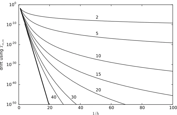
Figure 1. _{Drift in modified energy for the pendulum as a function}

of step sizehfor various values of m. The thick line indicates the limit.

are then chosen so thatU vanishes and that the trajectory passes close to (q1, q2) =

(0,0) before ending at some pointyT = (p1(T), p2(T), q1(T), q2(T)) where againU

vanishes. Carrying out that simulation the difference|H(y0)−H(yT)|is observed to beO(exp(−C/h)) whereC is some unspecified constant.

We repeated this experiment using our method, and found that in this case it had

zero error so the experiments we consider will not have this type of Hamiltonian. This matter warrants further investigations, but we have not pursued these in this paper.

6.1. The pendulum. In this experiment we apply the St¨ormer–Verlet method to the pendulum, which has HamiltonianH=p2_{/2−cos(q), integrated over the time}

interval [0,100]. Figure 1 reports the drift in the modified energy computed us-ing Tm,m for m = 2,5,10,15,20,30,40. Here, and in the other plots, the drift is defined as the difference between the maximum of the modified energy over the integration interval and its minimum. The figure suggests that the approxima-tionsTm,mconverge for this problem. The limit is indicated by the thicker line in the left part of the plot, which shows that the drift follows the exp(−c/h) behaviour predicted by the theory.

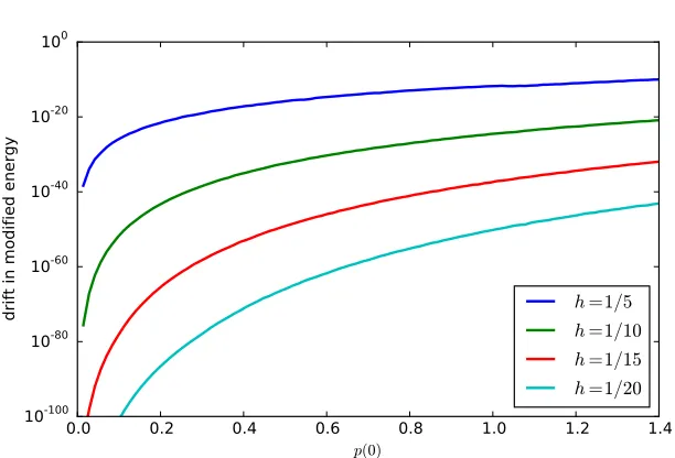
The initial value for the experiment reported in Figure1isq(0) = 0 andp(0) = 1. Next we study the effect of varying the initial condition. The result is shown in Figure 2. The St¨ormer–Verlet method shows improved energy preservation near the equilibrium point, revealing the exp(−c/hkfkD) dependency on step size and

0.0

0.2

0.4

0.6

0.8

1.0

1.2

1.4

p(0)

10

10

10

10

10

10

drift in modified energy

h =1/10 h =1/15 h =1/20

Figure 2. _{Drift in modified energy for the pendulum as a function}

of the initial momentump(0).

6.2. Kepler problem. The Kepler problem for one particle in a central force field is given by the Hamiltonian

H =1 2(p

2

1+p22)−

1

p q2

1+q22

.

We integrate over the interval [0,100] starting from the point

p1= 0, q1= 1−ecc,

p2=

r

1 +ecc

1−ecc, q2= 0.

where 0≤ecc <1 is the eccentricity of the orbit.

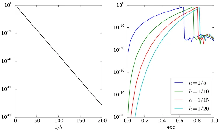
The left plot of Figure3 shows the theoretical exp(−c/h) behavior. In contrast with the pendulum, for this problem theTm,m do not converge asm→ ∞, but the sequence has to be truncated at a suitably chosen point. To find the optimalm, we approximate the error in them-th estimate as

|H−Tm,m| ≈ |Tm,m−Tm−1,m−1|. (6)

We compute this estimate form= 2,3, . . . ,200 and select the value ofmfor which the estimated error is minimized. This procedure recovers the expected exponential behaviour.

The right plot of Figure 3 shows the dependence of the drift in the modified energy on the eccentricity of the orbit. Almost circular orbits with a low eccentric-ity show much better preservation of the energy than highly elliptical orbits. An instability occurs at a critical eccentricity which depends on the step size. This can be explained by the fact the the topology of the energy levels of the modified energy changes withh, thus leading to unbounded trajectories and instability.

0

50

100

150

200

1/h

10

10

10

10

10

drift in modified energy

0.0

0.2 0.4

0.6

0.8

1.0

ecc

10

10

10

10

10

10

drift in modified energy

h =1/15 h =1/20

Figure 3. _{Drift in modified energy for the Kepler problem as a}

function of step sizehfor eccentricityecc= 0.6 (left plot), and as a function of eccentricity (right plot).

based on extrapolation [20] and a fourth-order scheme due to Blanes and Moan [3]. The last scheme is optimized for problems of the type we have considered. It has very small error coefficients at the cost of many stages, leading to coordinate errors which are typically three orders of magnitude smaller than Yoshida’s method at the same computational cost. The plots for the drift in modified energy of both Yoshida’s method and the Blanes–Moan method look the same as for the St¨ormer– Verlet method. In particular, the constant c in exp(−c/h) is the same. However, the drift in the modified energy for the St¨ormer–Verlet method is approximately a factor of three smaller than Yoshida’s method and a factor of four smaller than the method of Blanes and Moan.

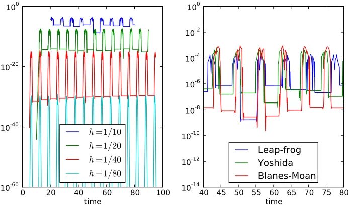
The left plot in figure4illustrates for several different step sizes how the modified energy varies. There are peaks when the particle is near the singularity at the origin. The crucial point is that the energy essentially recovers its value after this point before another close encounter. The plot on the right compares the three different methods. It is seen that the methods give rather different results, even though the maximal variation in the modified energy is almost the same for the methods. The Blanes–Moan method seems to preserve the modified energy better after the close encounter, which might indicate a special advantage of this method when applied to the Kepler problem. If, however, the time steps are scaled so that the computational cost is the same for the three methods, the St¨ormer–Verlet method will preserve the modified energy better than the high-order methods.

0

20

40

60

80

100

time

10

10

10

10

h =1/10 h =1/20 h =1/40 h =1/80

40 45 50 55 60 65 70 75 80

time

10

10

10

10

10

10

10

10

Leap-frog

Yoshida

Blanes-Moan

Figure 4. _{The difference between modified energy at a given time}

and the initial modified energy for the Kepler method with eccen-tricityecc= 0.6. The left plot shows the results for the St¨ormer– Verlet method for different step sizes, while the right plot shows the results for different methods. All methods are run with step sizeh= 0.1, so St¨ormer–Verlet does considerably less work.

indicates that information from the smooth parts of the trajectory is used near singularities, and that it might be important to use very high order approximations to get a clear picture of the drift. The graph also indicates that the algorithm can track instantaneous changes in energy.

Away from the parts of the orbit where the singularity at the origin is approached most closely, a lower value of m suffices. It is thus useful to find a more efficient method for finding the optimalminstead of computing the error estimate for allm up to some large value (here, 200). We found good results with the following ad-hoc termination criterion: compute the error estimate (6) for allmup to the first value ofmfor which

max

j=m−11,...,m−1|Tj,j−Tj−1,j−1| ≤j=mmax−10,...,m|Tj,j−Tj−1,j−1|,

and then choose the m with the minimal error estimate. The plots produced by this criterion are nearly indistinguishable from the plots produced when all mup to 200 are considered.

6.3. H´enon–Heiles system. The Hamiltonian of the H´enon–Heiles system is given by

H= 1 2(p

2

1+p22) +

1 2(q

2

1+q22+ 2q12q2−2₃q23).

Skeel et al. _{investigated the theoretical exp(−c/h) behaviour of the drift in the}

modified energy for this system, and report that the results are “less convincing” [5,

40

45

50

55

60

65

70

75

80

time

10

10

10

10

10

10

10

₀

50

100

150

200

Figure 5. _{The change per step in the modified energy (dashed)}

and the accumulated change (solid), and the optimal order m (capped by 200, marked by ’x’). The axis for the energies is on the left, which the right axis is for the orderm. This is for the St¨ormer– Verlet method applied to the Kepler problem withh= 1/20 and ecc= 0.6.

0 5 10 15 20 25

1/h 10-120

10-100

10-80

10-60

10-40

10-20

100

0.0 0.1 0.2 0.3 0.4 0.5 p1(0)

10-120

10-100

10-80

10-60

10-40

10-20

100

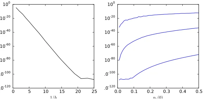
Figure 6. _{Drift in modified energy for the St¨ormer–Verlet method}

applied to the H´enon–Heiles problem as a function of step size h with initial conditionp1(0) = 0.1 (left plot), and as a function ofp1

arbitrary high orders. Figure 6 shows that the expected exponential smallness is indeed present, and that there is no problem in using the algorithm other than allowing for large values ofm(we again cappedmat 200). The effect of round-off error becomes visible when 1/h exceeds 20; remember that all computations are done with 120 digits.

The right plot shows how the maximal deviation of the modified energy changes as the initial condition forp1is varied; the initial conditions for the other variables

are fixed asq1 =q2 =p2 = 0. This plot shows that there is no abrupt change in

energy preservation when moving from regular, integrable motions (the region with energyH <1/12 or, equivalently,p1<1/

√

6≈0.4) to the chaotic regime of phase space (whereH >1/12).

We also applied the fourth-order methods due to Yoshida and Blanes and Moan to this problem, with the same results as for the Kepler problems: the St¨ormer– Verlet method shows slightly better energy preservation, but the value ofc in the exp(−c/h) dependence is the same.

7. Conclusions. We have supplied rigorous estimates for a numerical algorithm that computes the modified energy for methods based on operator splitting of Hamil-tonian systems. The estimate shows that the procedure can recover exponentially small estimates, known to exist theoretically. The estimates exhibit the same depen-dence on the important parameters ˜ry,handkfkD, and can therefore in principle

be used to extract their values from simulations. When comparing different split-ting algorithms, it seems that in the limith→ 0 the exponential remainder term only weakly depends on the method coefficients. Thus when considering the addi-tional cost of optimized, many-stage, methods these will have a larger drift than the second-order St¨ormer–Verlet algorithm. In other words, when it comes to pre-serving the modified energy, cheap, low-order methods are preferable. Although we have not considered ODEs originating from Hamiltonian semidiscretization of PDEs it seems likely that for long time simulations a low-order method such as St¨ormer–Verlet is preferable if energy preservation is important.

Appendix.

Proof of Lemma 2. Without loss of generality we assume thatn= 0. By representing (4) as a contour integral we have

Dmy(0) = 1 2πi

m

X

j=1

I

γ

(−1)j+1_(m!)2

hj(m−j)!(m+j)!

₁ z−jh−

1 z+jh

y(z)dz,

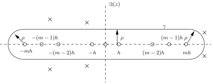
where the contour γ includes the points −mh, . . . , mh and excludes singularities ofy, as sketched in Figure2.

The derivative is given byy′(0) =₂1_πiH

γ

y(z)dz

z2 , so the error in the approximation becomes

Em(y)(0) =Dmy(0)−y′(0) = 1 2πi

I

γ

Km(z)y(z)dz, (7)

where the kernel is defined by

Km(z) =

(−1)m+1_(m!)2_h2m

Figure 7. _{The contour of integration used in the proof of Lemma2.}

Along the curveγ, the kernelKmachieves its maximum in modulus atz=iρ, and the maximum is

|Km(iρ)|=

(m!)2_h2m

ρ2_(ρ2_+h2_{)· · ·(ρ}2_{+ (mh)}2₎ =

1 ρ2_{(1 +} ρ2

h2)· · ·(1 +

ρ2

(mh)2)

= π

ρhsinh(πρ_h)

∞ Y

j=m+1

1 + ρ

2

(hj)2

where the last equality follows fromQ∞

j=1(1 +

ρ2

(hj)2) =

h

πρsinh(πρ/h). The product can be bounded as

log

∞ Y

j=m+1

1 + ρ

2

(hj)2

=

∞ X

j=m+1

log

1 + ρ

2

(hj)2

≤ Z ∞ m log

1 + ρ

2

(hx)2

dx≤ ρ 2

h2_m,

yieldingQ∞

j=m+1(1 +

ρ2

(hj)2)≤exp(

ρ2

h2m), and thus

|Km(iρ)| ≤ π

ρhsinh(πρ_h)exp

ρ2

h2_m

.

Since the length of the contour is 2πρ+4mh, the error expression (7) can be bounded as

|Dmy(0)−y′(0)| ≤

(πρ+ 2mh) exp_hρ22_m

ρhsinh πρ_h kykρ

where kykρ := sup_|ℑ(z)|<ρ|y(z)|∞. This upper bound is minimized by choosingm

so that d

dm(πρ+ 2mh) exp(ρ

2_/h2_{m) vanishes, i.e. m≈} ρ2

h2. This gives the bound

|Dmy(0)−y′(0)| ≤

e(π+ 2ρ2_/h2₎

hsinh πρ_h kykρ≤C1

ρexp −πρh

h2 kykρ

Proof of Corollary3. This follows from

|H(pn, qn, tn)−Tmn∗,m∗| ≤12|q

T_(p′_−D

m∗p)|+1₂|pT(q′−D_m∗q)|+1₂|β′−D_m∗β|

≤1

2|qn|1kp′−Dm∗pkρ+ 1

2|pn|1kq′−Dm∗qkρ+ 1 2kβ

′

−Dm∗βkρ

≤C1ρexp(−

πρ

h)

2h2 (|qn|1kpkρ+|pn|1kqkρ+kβkρ)

where the last inequality follows from Lemma2.

Proof of Lemma 4. We prove this by Picard iteration: set ˜x1 = xn and iterate ˜

xk+1(t) =xn+R t

0g(˜xk(s), s)ds. Fixt∈ Dt, and assume at first thatrtis sufficiently

large. For ˜xk+1,x˜k ∈ Dy

|g(˜xk+1, t)−g(˜xk, t)|∞

= Z 1 0 d dsg ˜

xk+1+s(˜xk−x˜k+1), t

ds ∞ = 1 2π Z 1 0 I

|z−s|=R

g x˜k+1+z(˜xk−x˜k+1), t

(z−s)2 dz ds

∞ = 1 2π Z 1 0 I

|w|=R

g x˜k+1+s(˜xk−x˜k+1) +w(˜xk−x˜k+1), t

w2 dw ds

∞ .

The radiusRis restricted by the requirement that the argument ofglies withinDy or

|x˜k+1+s(˜xk−˜xk+1)−xn+w(˜xk−x˜k+1)|∞

≤ |x˜k+1+s(˜xk−x˜k+1)−xn|∞+r|(˜xk−x˜k+1))|∞

≤ |t|kgkr+R|x˜k−x˜k+1|∞< ry

by using

|x˜k+1+s(˜xk−x˜k+1)−xn)|∞

≤ sup

|τ|=|t|

Z τ

0

(1−s)|g(˜xk(τ), τ)|∞+s|g(˜xk−1(τ), τ)|∞dτ

≤ |t|kgkr.

We may therefore choose

R=η ry− |t|kgkr

|x˜k+1−x˜k|∞

, 0< η <1

which gives the supremum-norm Lipschitz bound

|g(˜xk+1, t)−g(˜xk, t)|∞≤ k gkr

η(ry− |t|kgkr)| ˜

xk+1−x˜k|∞.

Let ∆k+1(|t|) = sup_|τ|=|t||x˜k+1(τ)−x˜k(τ)|∞, then the Picard iteration ˜x1 =xn, ˜

xk+1=xn+R t

0g(˜xk(s), s)ds, converges if ∆k→0 ask→ ∞, with

∆k+1(t)≤

Z |t|

0

kgkr

η(ry−skgkr)

Introducing the generating functionG(µ,|t|) =P

k≥1µk∆k we have

G(µ, t)≤µ|t|kgkr+µ

Z |t|

0

kgkr

η(ry−skfkρ)

G(µ, s)ds.

Since the terms in this inequality are positive, an upper bound is the solution of dG+_(µ,|t|)

d|t| =µkgkr+

kgkr

η(ry− |t|kgkr)

G+(µ,|t|), G+(µ,|t|= 0) = 0,

i.e.

G+(µ,|t|) = µηρ η+µ

1−|t|k_rgkr

y

−µ/η

−1−|t|k_rgkr

y

.

BecauseG+_{is analytic inµaroundµ= 1 provided|t|<} ry

kgkr, the sequence ∆k(|t|) converges uniformly to zero and hence ˜xk(t) convergesuniformly to the solution. Since each iterate ˜xk+1(t) = xn +

Rt

0f(˜xk(s), s)ds is analytic in t ∈ {t ∈ C : |t| < min{ ry

kgkr, rt}} the uniform convergence gives by Weierstrass theorem that y(t) = ˜x_∞(t) is analytic in this domain as well.

Proof of Theorem 5. In Theorem 1 we take g =f, thus kgkr ≤ ₁₋2_ηkfkD with f

analytic inD′. This gives that they(t) is analytic in the domain

(

τ∈C_{:|ℑ(τ)|<min} r˜y−δ

2 1−ηkfkD

, ηδ ekfkD

!) .

We find that the bound is optimized by picking ˜ry =ηδ where η = _ee−2

−√2e. Thus we may takeρ=_ekηδ_fk

D <0.6835

δ

kfkD in Corollary3giving the exponentially small

bound (t=nh)

|H(pn, qn, t)−Tm∗,m∗| ≤

C1

2h2exp

−C2

δ hkfkD

(|qn|1kpkρ+|pn|1kqkρ+kβkρ),

whereC2= 0.6834π.

REFERENCES

[1] G. Benettin and F. Fasso. From Hamiltonian perturbation theory to symplectic integrators and back.Appl. Numer. Math., 29:73–87, 1999.

[2] G. Benettin and A. Giorgilli. On the Hamiltonian interpolation of near-to-the identity symplectic mappings with application to symplectic integration algorithms. J. Stat. Phys., 74(5/6):1117–1143, 1994.

[3] S. Blanes and P. C. Moan. Practical symplectic Runge–Kutta and Runge–Kutta–Nystr¨om methods.J. Comput. Appl. Math, 142(2):313–330, 2002.

[4] M. P. Calvo, A. Murua, and J. M. Sanz-Serna. Modified equations for ODEs. In Chaotic Numerics, volume 172 ofContemp. Math., pages 53–74. Amer. Math. Soc., Providence, RI, 1994.

[5] R. D. Engle, R. D. Skeel, and M. Drees. Monitoring energy drift with shadow Hamiltonians.

J. Comput. Phys., 206(2):432–452, 2005.

[6] E. Hairer and C. Lubich. The life-span of backward error analysis for numerical integrators.

Numer. Math., 76:441–462, 1997.

[7] E. Hairer, C. Lubich, and G. Wanner.Geometric Numerical Integration. Structure-Preserving Algorithms for Ordinary Differential Equations, volume 31 ofSpringer Series in Computa-tional Mathematics. Springer, Berlin, 2002.

[8] L. O. Jay. Beyond conventional Runge–Kutta methods in numerical integration of ODEs and DAEs by use of structures and local models.J. Comput. Appl. Math, 204(1):56–76, 2007. [9] B. Leimkuhler and S. Reich.Simulating Hamiltonian Dynamics. Cambridge University Press,

[10] J. E. Marsden and M. West. Discrete mechanics and variational integrators.Acta Numerica, 10:357–514, 2001.

[11] P. C. Moan. On the KAM and Nekhoroshev theorems for symplectic integrators and impli-cations for error growth.Nonlinearity, 17:67–83, 2004.

[12] P. C. Moan. On rigorous modified equations for discretizations of ODEs. Technical Report 2005-3, Geometric Integration Preprint Server, 2005. Available fromhttp://www.focm.net/ gi/gips/2005/3.html.

[13] P. C. Moan. On modified equations for discretizations of ODEs.J. Phys. A, 39(19):5545–5561, 2006.

[14] S. Reich. Backward error analysis for numerical integrators. SIAM J. Numer. Anal., 36(5):1549–1570, 1999.

[15] Z. Shang. KAM theorem of symplectic algorithms for Hamiltonian systems.Numer. Math., 83:477–496, 1999.

[16] R. D. Skeel and D. J. Hardy. Practical construction of modified Hamiltonians.SIAM J. Sci. Comput., 23(4):1172–1188, 2001.

[17] R. D. Skeel, G. Zhang, and T. Schlick. A family of symplectic integrators: Stability, accuracy, and molecular dynamics applications.SIAM J. Sci. Comput., 18(1):203–222, 1997.

[18] P. F. Tupper. Ergodicity and the numerical simulation of Hamiltonian systems. SIAM J. Appl. Dynam. Systems, 4(3):563–587, 2005.

[19] J. Wisdom and M. Holman. Symplectic maps for then-body problem: Stability analysis.

Astron. J., 104(5):2022–2029, 1992.

[20] H. Yoshida. Construction of higher order symplectic integrators.Phys. Lett. A, 150(5–7):262– 268, 1990.

E-mail address:[email protected]